Aeolian Transport and Vegetative Capture of Particulates
by
John W. Glendening
P.r. Peter C. Sinclair
Department of Atmospheric Science
Colorado State University
By
John
w.
GlendeningPreparation of this report has been financially supported by
AEC (ERDA) Grant #5594605
monitored by the Lawrence Livermore Laboratory
Department of Atmospheric Science Colorado State University
Fort Collins, Colorado May, 1979
ABSTRACT
AEOLIAN TRANSPORT A.T\ffi VEGETATIVE CAPTURE OF PARTICULATES
Aeolian (wind-blown) transport of soil particles to which plutonium is attached is responsible for the escape of radioactivity beyond the boundaries of the Nevada Test Site. This thesis concerns the hori-zontal aeolian erosion of the large particles, which travel close to the ground. They are captured by desert creosote bushes, building radioactive wind hummocks around the shrub bases.
The airflow above and below the average shrub height and inside a bush is investigated. The drag coefficient above the vegetation is found to decrease with increasing wind speed. Below the shrub height, the development of an internal boundary layer results in a logarithmic velocity profile. The bushes are widely spaced and aerodynamically very porous, producing a flow more typical of
individual roughness elements than of a plant canopy. Partitioning the total drag above the vegetation into ground drag and bush drag contributions illustrates the dominant role of the vegetation in producing drag and thereby controlling soil erosion.
The yearly horizontal erosion flux below bush height is estimated to be 40 grams per year per cm width, based upon monthly wind and soil moisture data and field erosion measurements. The ground stress needed to initiate movement is close to the minimum stress determined by Bagnold. Under these low erosion conditions the bush hummocks cannot grow large enough to significantly affect the
ground strass inside the bush, so the limit to hummock growth is the creosote bush life span. It is concluded that the larger eroding
transport.
John W. Glendening
Department of Atmospheric Science Colorado State University
Fort Collins, Colorado 80523 Fall, 1977
ACKNOWLEDGEL~NTS
The author expresses his sincere appreciation to his advisor, Professor Peter C. Sinclair, for his support and advice throughout the prepartation of this thesis. Thanks are also expressed to Dr. Robert N. ~eroney, for his suggestions and encouragement, and to Drs. Jack E. Cermak and Elmar R. Reiter for reviewing this work. Messrs. Norm Kennedy, Ralph Quiring, and Don Homan provided data which was incorporated into this thesis. Appreciation is also extended to Drs. C.W. Ferguson,
A.
Klute, R. Moses, andF.
Wentfor their helpful discussions. I am indebted to Ms. Julie Wilson for typing this manuscript.
This research was sponsored by AEC (ERDA) Grant #5594605 which was monitored by the Lawrence Livermore Laboratory.
ABSTRACT . • • •
ACKNOHLEDGE..'1ENTS
LIST OF TABLES . •
LIST OF FIGURES . .
LIST OF SYMBOLS . •
i i iv vii viii x 1. 2. 3.4.
5.6.
INTRODUCTION.
NEVADA TEST SITE DESCRIPTION • . .
2.1 Climatology • • •2.2 GMX Area . . • • 2.3 Test Bush Site. 2.4 Vegetation . • 2.5 Soil . • • . • • 2.6 Bush Hummocks ••
EXPERIMENTAL MEASUREMENTS
3.1 Field Instrumentation . . • • • • • 3.2 Hot Wire Anemometer Data Analysis.
AIRFLOW ABOVE AND WITHL\j' VEGETATION •
AIRFLmol MEASUR.E.L'1ENTS. • . • . • •
5.1 Flow Above the Vegetation. 5.2 Flow Below Shrub Height . . • 5.3 Flow Inside the Test Bush. 5.4 Drag Partition.AEOLIAN EROSION • • •
1 3 5 5 8 11 18 24 27 27 29 34 45 45 49 56 59 67 6.1 6.2 6.3 Erosion Description. Soil Erosion Factors • Erosion Flux Formulae. •67 71 74
7.
EROSION ASSESSMENT . .
7.1 Threshold Stress
7.2 Erosion Flux Formula Calibration.
7.3 Yearly Erosion Flux Calculation . . . • • •
v
76 76 80 89
TABLE OF CONTENTS (cont'd)
Page 8.
9.
VEGETATIVE CAPTURE. . . • . . 8.1 Shrub Interception of Particles.
8.2 Estimation of Ground Stress Inside the Test Bush
8.3 Hummock Growth .
8.4
Transport of Radioactivity SUMHA..J:tY 102 102 104 107 110111
BIBLIOGRAPHY • . 114APPENDIX A: EFFECT OF ~1EAN AJ.'ID FLUCTUATING VERTICAL VELOCITY ON
MEASURED HORIZONTAL VELOCITY. • . • . • . . . 123 A.I Error Due to Non-zero Mean Vertical Velocity
A.2 Error Due to Vertical Velocity Fluctuations . • APPENDIX B: STRESS ESTIMATION FROM AN EQUILIBRIUM LAYER
AS SUMPTION . . • . . . • . • B.1 Flow Between Shrubs. B.2 Flow Inside a Bush . •
APPENDIX C: STRESS ESTIMATION FROM TURBULENCE INTENSITY MEASURE.1I1ENTS . • . • . • . • . . . • . • . • vi 123 124 125 127 133 136
Creosote Bush Measurements 15
GMX Monthly Erosion Estimates. . . 100
Caption Page
Desert Pavement Soil Analysis. 21
23 82
SYSTRAC Station 15 Climatalogieal Winds. 92 Wind Hummock Soil Analysis . .
GMX Aeolian Erosion Measurements
SYSTRAC Station 15 Winds for Erosion Calibration
Periods. . • • • • . . . • •• 87
(U*) g Estimates Inside the Test Bush 105 (U*) /U and (U*)
/0-
Between Shrubs at 4 emg g u
Height . . . • . . . • . . . 131 Nevada Test Site 10 Year Climatological Summary
(1962-1971). . . 6 Table No. 1 2 3 4 5 6 7 8 9 10 vii
LIST OF FIGURES
Creosote Bush with Wind Hummock at GMX Area. . 17
Test Bush Site at GMX Area 10
Wind Profile at the Center of the Test Bush. • 60
Profile of the Test Bush Hummock • . 25
4
13
90 Page Caption
Nevada Test Site (NTS) Locations
Creosote Bush Growth Rate.
Periods. . . . 4' • • • • • • •
Wind Profiles Near and Inside the Test Bush. . 58
Airflow Regions Behind a Windbreak • 40
Wind Profiles Above and Below Shrub Height 53
Wind Profiles Between Shrubs . 50
Soil Structure of the Desert Pavement. 19
Meteorological 8 m Drag Coefficient as a Function
of Wind Speed. . . • . • 48
NTS Wind Speed in Miles per Hour as a Function of
Time of Day. . . • . • . . 7
Radioactivity Isopleths at Gl1K Area. . 9
SYSTRAC Station 15 Complement Cumulative Wind Frequency Distribution for Erosion Calibration
Saltation-produced Dust Episodes 79
NTS Wind Direction Percentage as a Function of
Direction for March. . • • • . • . 84
Threshold Velocity Estimate from Dust Episodes 81 Threshold Friction Velocity as a Function of
Particle Diameter. . • • . . . 77
(U*)~/U and
(U*)g/cr
u Between Shrubs as a Functionof W~nd Speed. . • • • . • • . • . • . . . • . 55 Figure No. 1 2 3 4 5 6 7 8 9 10 11 12 13 14 15 16 17 18 19 20 viii
Figure No. 21
Caption
Erosion Flux Equation Calibration
Page 91 22
23
Soil Moisture as a Function of Relative Humidity. 95 Relative Magnitude of Terms in the Turbulent Kinetic
Energy Equation . . . • . . . 128
Symbol A s D D o d E F F d F m g H
~
K m k L M M (15 atm) nLIST OF SYMBOLS
Definition Ground area cuvered by shrubShrub frontal silhouette area
C=
DH) Saltation mass concentration at heightz
Surface meteorological drag coefficient
C=
U*2/U2)Surface aerodynamic drag coefficient Meteorological drag coefficient of individual shrub
Shrub diameter
Zero plane displacement height Particle diameter
Empirical constant in erosion flux equation
Horizontal erosion flux Drag force
Vertical momentum flux Gravitational acceleration Shrub height
Eddy heat transfer coefficient Eddy momentum transfer coefficient von Karman constant
Monin-Obukhov scaling length Moisture content of soil
Soil moisture content at 15 atm suction Frequency x Dimension L L L
MT
3
/L
3
M/LT
ML/T2 ML2/T2 L/T2Symbol
Q
Definition Frequency of SYSTRAC winds Mean atmospheric pressure Erosion wind factor
[. En. U. 2 CU. - U t)] • ~ J. ~ J. Dimension q R Ri RH S S Cn) u T U (z) U. ~ U meas U t U* (U*) g (U*)t Ll(U*)t u u* V W (z)
Mean kinetic energy of turbulence Gas constant
Richardson number
Relative humidity of air
Specific area per bush L2
Spectral density function L2/T
Mean air temperature
a
Mean horizontal wind at height z LIT Mean of SYSTRAC velocity interval LIT Total velocity measured by hot wire LIT anemometer
Saltation threshold velocity LIT
Surface friction velocity (=
Tip)
LITo
Surface friction velocity of ground LIT
(= 't" Ip)
g
Saltation threshold friction velocity LIT Threshold friction velocity increase LIT due to non-zero soil moisture
Fluctuating horizontal velocity LIT
Friction velocity C=
Tip)
LITMean transverse veloc ity LIT
Mean vertical velocity at height z LIT
Symbol W max w x
z
o z z or
y e:a
p cr cr u L oLIST OF SYMBOLS (contld)
Definition
Estimated maximum of vertical velocity Fluctuating vertical velocity
Horizontal distance
Characteristic roughness length above vegetation
Vertical distance
Characteristic roughness length of ground
Kolmogorov one-dimensional constant Adiabatic lapse rate
Diabatic correction to equilibrium equation Height of internal boundary layer
Viscous dissipation of turbulence Monin-Obukhov dimensionless height
(= z/L)
Fluctuati~g air temperature Roughness element concentration parameter (= Af/S)
Kinematic viscosity of air Density of air
Density of particle Standard deviation
RMS velocity variation (=
~)
Shear stressTotal surface shear stress above vegetation (= L
b
+
Lg)Surface stress due to vegetation
xii Dimension
LIT
LIT
L L L LaiL
a
LIT
ML2/T2 ML2/T2Symbol
t"
g
~
Definition Surface stress due to ground Moisture potential of soil Shrub porosity
Diabatic correction to logarithmic wind profile
Foliage area per unit volume
Dimension
L
L
Any
other symbol not listed here is explained whenever it appears.1. INTRODUCTION·
Releases of radioactive plutonium have contaminated soil on the Nevada Test Site (NTS). Aeolian (wind-blown) transport of ?articulates with attached plutonium is responsible for the escape of this toxic element beyond the NTS boundaries. The transport is believed to
occur mainly through resuspension, small (diameter < 80 ~m) contaminated particles being lifted vertically and then moving with the wind. This thesis examines the horizontal transport of the larger contaminated particles which cannot be resuspended by turbulence, i.e.
wind erosion.
On the Nevada Test Site the wind loosens, picks up, and transports contaminated soil particles comprising the desert pavement. Creosote bushes capture the eroding particles, building hummocks up to 20 cm high under the bushes. These wind hummocks are more radioactive than
the surrounding soil.
This thesis considers the yearly erosion flux and the capture of loosened material by the vegetation, as well as the airflow so
important to both processes. Wind profiles .above and helow bush height and inside a bush are obtained. This allows the partitioning of the total drag into the drag on the bushes and the drag on the ground. The latter causes wind erosion, and this partitioning measures the effectiveness of the vegetation in reducing erosion. The threshold surface stress needed to dislodge the soil particles is. determined, The magnitude of the desert erosion flux is estimated from wind data, based upon actual field measurements with corrections for soil moisture factors. Finally the effectiveness of the shrubs
in capturing the eroding particles, the resulting mound growth rate, and limitations to hummock growth are discussed.
2. NEVADA TEST SITE DESCRIPTIO~
The Nevada Test Site (NTS) encompasses an approximately rectangular area 50 miles (N-S) by 30 miles (E-'i-l) in southern Nevada, 65 miles
northwest of Las Vegas (Fig. 1). The terrain is extremely irregular, consisting of generally north-south ridges and valleys with a north to south downward slope. The valleys consist of gently to moderately sloping alluvial fans and terraces. The climate is typical of the Great Basin desert with high midday temperatures and low precipitation, producing typical desert vegetation.
The U.S. Atomic Energy Commission conducted nuclear explosions at NTS between 1951 and 1963 using plutonium (Pu239) in both critical and subcritical configurations. Some of this radioactive plutonium has moved outside the NTS boundaries (Bliss and Dunn, 1971). The primary source of this escaped plutonium is believed to be the so-called "safety" explosions designed to test the effects of an accidental detonation of the high explosive trigger of a nuclear bomb. These explosions scattered large amounts of plutonium. Neither the accidental ventings of underground explosions nor the release of unfissioned plutonium from above ground full scale nuclear explosions are considered to be major sources of escaped plutonium. The movement is mainly by aeolian (wind-blown) transport with water transport playing a secondary role (Eberhardt and Gilbert, 1974). The escape of plutonium, a very hazardous toxic element with an
extremely long half life, beyond the confines of federally controlled land is important because it raises the possibility of human health
'M .1. Fig. 1. Nevada Test Site (NTS) Locations (after Quiring, 1968)
,I I,''' : I I . i [ . j J •
.:t \ .
...
c' .."-l\'7 " .J \, : '.... ,"5
damage from inhalation of resuspended plutonium or from injestion of plutonium picked up by plants or animals in the food chain.
2.1 Climatology
The climate of the NTS area is typical of a high desert basin with large temperature variations, predominately clear skies, and low
relative humidities (Table 1). The average daily temperature range is about 50°F on a clear dry day in summer or autumn. The temperature can reach an extreme of II0oF. The annual average precipitation is about six inches. The rainfall maximum occurs in January and February, tapering off to a pronounced minimum in June. It then rises to a
secondary maximum in July and August, followed by a rapid decline to a secondary minimum in October and a rise to the winter maximum. The wind regime is typical of mountain-valley terrain. Southerly winds predominate during daylight hours during the warm half of the year. In winter, by mid-day there is sufficient heating on the mountain slo~;s to introduce a southerly component. Westerly to
northeasterly winds prevail at night during all months. The strongest winds occur during the spring. The wind speed shows a strong diurnal effect, peaking at 1500 hours (Fig. 2).
2.2 GMX Area
The experimental observations for this thesis were made in the GMX area of NTS. It is a region about 1 km square located within the much larger Frenchman Flat region (Fig. 1). GMX is generally flat at an elevation of 910 meters. The elevation increases slowly to the north and the area is crossed by shallow stream channels
LATITUDE 36" 57' N LONGITUDE 116" 03' W
ELEVATION 3.924 Feel YUCCA FLAT. NEVADA- NEVADA TEST SITE
NEVADA COOROINA TE SYSTEM (CenlfOll
E680.875 N803.600
TEMPERAT~RE reG~EI"fl DAYS
'"
~;v£~s=r=
[XTTO£S ~~o
PRECIPITATION
(lnchu) AVERAGE NUMBER OF DAYS, - - -
-, .... Sunwl P'U.C.rtIAHOH I TEMPfNAIUH(
"I- S Ul
~~ l:i oil . . ~ oil 15 ~ ..IU' ....1fI~1I... _1
~a
6~ ~ ~ ~
It g~
::: m-t-:M~ d bbti~l~E~.J..; ~!f!!fr~Eif.n~O~~bob ~ :1 « lr 5 E 5 0 ~ 5 ::- ~ ~ ~. "! I:>.:)~ ~
_J 0 a~
0 0 7'C 0 N r\t • __ ..~ U 0: U - . -.,; __ f- 0'1 I'") fill 0 t-m...
3 'i '"...
~ ffi ~ ZHJ2I"-14 PST psr STATION .5l1LtAld' ~~SSUR£ I 'O;':SoI_ ~~--~ ~ WINO ... (Speed~tnmph) ~ ~ n m ......
...
... ~ m '" "...
..
~ ~ IlOUR ....hc.:s'....,n-a ---,--,-,--"fLA'IV£ ...DlJY....
04110 116 122 '" ~i
~
ffi '" ~ SHOW:1I1:~
: !i~ ... " ' 0 ~ ~:i '"..
...
>-~a
t-m...
Ii...
ffi ~..
~ :J: ~ :iS
...
J '"..
...
..
t-~~ . . t-m~...
'"..
'"...
:i..
z d 8..
zE
:r '" ~..
i
9 '"..
~ ,-t: :J: C> i' ~ :J: t-5 :i ~ >-:i ;i~ 0 , " HI :i T >-~ H ~~ xI:I.:I~ I~I-~
21.4101.10 II~.1~_~24~~ o 0 12 0 o 2 0 .- --_. ._-
.---_._-
--_.. - _ . --~._._.- -.- ._-- -.. - ..- .... JAN- 52.'_. - - - - -- - - -- ._. ----20.8 36.5 n '971 ·2 1910 071 0. - _.- - - -~ 4.(12 1969 r - - - - ._- -1911. 1.25 1969 0.9 4.3 19624.3 1962 61 49 l5 60 66 ~O 1965 3111d= 26.'0 26.54 25.42 4.9 Il 0 10 2 I X • ~~---"=- - _. =- - _. - - ._-- - _ ..- - -_.I!~ ~.! 3~:.a 4~~!!. ~_ ~ 'J/I~ 662. _~ _~~.l~5 !~ !_196/.~~ 1969~..a..!:~ _~"?_ ~..~. ~~ 6!....~~ ~ ~ .~ ~~. ~~. ~II~ ~ ~!!~ ~~~5.0 ~. _~ .~ ~.! ~ "
~
. 60.9 ~1,! ~~.:~II.' I~_~ 196~ ~~ ~ _~.•_~~ !~~ ~ .'?~. ~ .~~ 2D ..!.:~_.~ _4..~'969 ~...!'.._~_~. ~.~_ ~ I~!~ ~~~ 2~99 ~4; 25.4~4.0 ~_..!..!.<: _~...!. ~ 0APR 6/.8-- _.--34.4 -_._.51.1 -O<J. _ -.962- -13 .966- - _ .411 - -I 45 2.57 1965 T- _._.962..-..1.00- ._-1963 0.7- , -3.0 - -1964 _.3.0 1964 t52---- - ' - -21 -·21 30 9.1 60. 1910 '5G'2.<--- - - -9llI5J25.96 26.39- -
2~.50
4.5- _._.Il 9 U 3 --_., x"I"
_.. ~! 18.9 ~,l.~ ~.~.~.~~ ~~.~~-,~?__
~__
~~_~~_1?7' _!_!~~~ .Ilb 19710 I '9.~.!..1~~~..3~. I/~I ~~!?:il _ _ 1_ _25.94263925.41.~14 "_~ 2~~..~..~.JUN 816 4'19 60.0 101 .I~~ .~ r~!~ _.~~ 1M __~~_ II~. 196~L ~~~. _.~~ I~~.~ _~ 0 . ~.?. ~ _~26 If! ~~2 '0!i\9JlMl2~592 ~~~ !-i.~ ~..'9.. __! .4..!_ -'- _(J. ~. 0
~ ~ g,!i!'~
:;;;~£ ~~...;- -=~~._~
.
;-~F:..l!.. ~96~ .nl~~~.~_
-
0-~
__;:. . . - 40 20 ;;::~ ~iLi ,~~;
~600 .~~.~
.
.lcll!~
9~.~
..3_.~
0 .(J!,IJG~~E _~!,I _~~ ~ 1910_~ 196~._.!.. ~ .34 104; 1965~ 19f.2 .1:> 1911!..l!.._~ . ..l!.. .~.'!. .~~ ~ .~~~! 1~08 ~~21i00~ ~~.:1.0~~ 11.. ~ 3 ..L(J E.(J
SU'
864 461 665 10~19/ • .3~.!'!i!. ~ .~~~II.. s18-~'! .~_ 196111_2.13 ~'! O_~.. _ .. O n _ ~.~..~.!.!...E. !E.5~ .~~ ~~~~6.00 ~ ~..5~3.:.!..~~..~ _~_ 2 1 1 " 0 OCI .?~..~C'. .~~ ~ 19fA! ~ 1911 r21i6 _!.~ ~ 196,! _0_ I~?!,_42.~~_.~ ._,-. .191' . ..!. ~_ ~ ~. ~. ~ ~ ~ I~~ ~}1.3ilI1126.OG~~ ~.5~ ~ ~() !. • I I 0 0 0~
l!!..!!!~ '!.~]
11.5"62I--'~
19661602~
__ .7'~.'965
...~
'962 LIO 19/0 05~!!
.. 19£.4.~,~ ~~ ~!
3..'!..~!.. ~. ~!. ~!. ~.~ 2~1~
£'6.00~~. 2~.64
4.8 .3!'~ .~
2 • "-_Off 507 19.9 :i5} {O f.)L4 -1111967 _!~4 ~ :?9 ~~_ 1965.!..1%91_.~~ ~.~ ~~_ ~ ~~?I ?:~ _~~.!._68 ~ ~.!..- ~~:! .~ .~~~ ~KY.VlO26.01.26~~ ~~:~ 4.6 ~4 6 _~ 3 I _..!_ K
41 ;>'310 .127 II )\ 2 • 0 " 0 010 0'\ _)12.51
~~~J~~~~~I~1:~t~J~m~;~J~;llt~'d~~1;t:~I:l~~!M~~~~~1254~L~9~1~1~~~L:iLL~
1~~I~El~
)t ~ ca~ ~.H_'''I''I''lUallllll_'''M''''li~I''D.~.'.• lU!i1 .U.It ..'UIII'U 1I.U.ICU.
... I\Ao.lI'll'lIUI.jl\lt lJ't\A\U1U IIIlll ...u..n
... 1. "'''''lIIll'D'hril.ll''''IoSUI:.
~. ~ .\011"....!J1l ... , ... ill "'llll "Nlla~laau..., H'" 1,. tlllIllta_lWoal_ II • • • S11I.-1
, Ifill A'loII'V.IfCM"1t I. fHI • •U I'AJI,~. , I""
(W ..n(:M.I~ILnl-'~':II" t.t.&I'IO'~I· i:tl~ ;·.l!."~!" ~"I~lil'l"ll:I1I""".'lI1lt:"''&''
7 00 03 06 09 12 15 18 21 24 a 8 9 10 9 JAN JAN 9 FEB 10
"r
FEE MAR [ : I APR 10 10I
I
MAY 9I:
~"AY
JUN JUN JUL lJUL I AUG s :l
i AUG!
I 1 9 I 9 SEP SEP OCT OCT NOV NOV DEC DEC 9 JAN a s 9 10 9 JAN 10 " I I i I I I 00 03 06 09 15 18 21 24 HOUR (PST)Fig. 2. NTS Wind Speed in ~liles per Hour as a Function of Time of Day (from Quiring, 1968)
with a broad southward drainage. Low wind hummocks are found around the bushes.
From December 1954 to February 1956 22 small high explosive "safety" detonations released a few curies of plutonium. The area of measurable
2
contamination is about 0.12 km , surrounded for several kilometers by a region of similar terrain and vegetative cover. This "safety" explosion region has frequently been used to study the plutonium escape problem. Anspaugh et al. (1976) investigated the wind-induced resuspension of plutonium contaminated soil particles, and Sinclair
(1976) estimated the downwind transport due to dust devil activity. Soil (Tamura, 1974), vegetative (~omney et al., 1974), and animal (Smith, 1974) removal have all been studied in this area.
Environmental weathering over the 20 year period following the plutonium releases has intimately associated the plutonium, in the form of plutonium oxide, with host soil particles. The plutonium activity spread from ground zero downwind in the prevailing wind direction as the contaminated soil particles were dislodged and transported by wind forces, resulting in an elongated radioactive isopleth pattern (Fig. 3). Thus the radioactivity moves principally through aeolian transport of contaminated soil particles.
2.3 Test Bush Site
The primary wind measurements were made at a sire on the western edge of the GMX area because of the presence of a previously estab-lished meteorological tower (Fig. 4). The site was located on an alluvial fan sloping southward with a gradient of 1-2%. It was surrounded by evenly spaced vegetation with an upwind fetch of over
9
o
200
!FEET
ISOPLETH 1
c:::::J
500-5000 CPM
2
hj'-.:-::!)5000-25,000 CPM
3
!iiiiiI 25,000-50,000 CPM
4
~,,\,,'.'I>50,000 CPM
5
c::::J 0-50,000 CPM
Fig. 3. Radioactivity Isopleths at G}fX Area (from Gilbert and Eberhardt, 1974)
11
12 km to the south-southwest. This is the prevailing wind direction for the daytime high wind periods and also for the measurement periods.
At this site a test bush was chosen for extensive air flo~.
measurements close to and inside the bush. The criteria for choosing this bush were:
1) This test bush had a very large wind hummock built up inside it (18~ cm). Studying such a large hummock might provide clues regarding a size limit to hummock growth. 2) There was a large spacing between this bush and the
closest upsteam bush. This allowed the wind incident upon the chosen bush to be in approximate equilibrium, which would not be achieved if the air flow approaching the bush was disturbed by the presence of another bush a short distance upWind.
3) The test bush was large in diameter and thus exerts a greater effect on the incident air flow than a small bush. This reduces three-dimensional effects, reduces the effects of the wind measurement probes on the air flow, and allows the hot wire anemometers to be spaced further apart inside the bush.
4) The test bush was within ten meters of a meteorological tower. It was also very close to a bivane which could be used to determine the prevailing wind direction, needed to align the hot wire anemometers.
2.4 Vegetation
The vegetation in the GMX region is predominantly creosote bush (Larrea divaricata or, in older texts, Covillea tridenta) with
various coexisting species, the specific species varying in different regions of the GMX area (Rhoades, 1974). Creosote bush is a shrub with an average height of 0.6 m in the GMX area. Its main stems are woody, rising at an angle from the ground. They are limber with a one cm maximum diameter. The branches can be either simple or branched, becoming bushy at the tips where the stalk diameter
3-4 mm wide broad leaflets joined at the base. Excretions of the lac scale are deposited in great quantity on the stems. It is fed upon by only a few insects, occasionally by jackrabbits, and is considered a "noxious weed." The creosote bush grows well on all soils and is the dominant plant for 30 million acres of the southwest United States.
The creosote bush growth rate is mainly determined by the
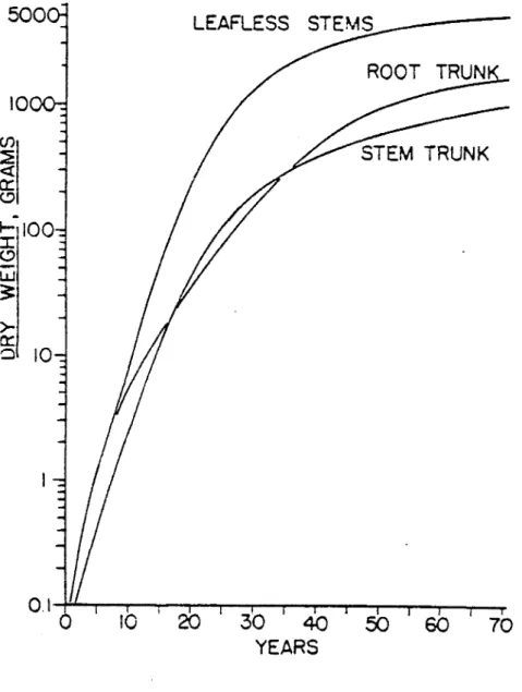
annual precipitation (Dalton, 1961). The shrub grows until its size is limited by the available water. The low desert precipitation accounts for the wide spacing and even distribution of the GMX creosote bushes. Chew and Chew (1965) experimentally determined the age to reach
mature growth as about 50 years. The volume of the branches increased linearly with age from 20 years until maturity (Fig. 5). Unfortunately the dependence of shrub height and diameter on age were not determined.
The average life span of a creosote bush is uncertain. No
definitive studies have been made and only estimates from experienced desert observers are available. Dr. Fritz Went of the University of Nevada estimated the average lifetime to be about 100 years, but he remarked that the definition of life span is of importance since during periods of drought the branches die, leaving the root which may later grow new shoots during favorable conditions (personal communication). Dr. C.W. Ferguson of the Douglas Tree Laboratory, University of Arizona estimated the average life span as 50 to 100 years (personal communication). Shreve, a lifelong observer of creosote bushes in Arizona, estimated the average life span to exceed 100 years (Shreve and Hinkley, 1937). The average estimate is thus about 100 years.
13 )
-a::
~10
10
LEAFLESS
20
50
60
70
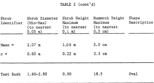
Rhoades (1974) found the sizes of the creosote bushes to vary widely between different regions of the ~1X area. The southeast sector had three meter high bushes, while others had bushes less than one meter high. Measurements of 20 creosote bush clumps close to the chosen test bush found the average height (H)' to be 1.06 m, the
variability being relatively small (0
=
.22 m) (Table 2). The average "diameter" (D) was 2.07 meters (0=
0.10 m), "diameter" being the average of the longest and shortest widths of the bush. The bush shapes ranged from circular to irregular oblongs. Most of the creosote bushes were in clumps of what appeared to be 3-4 bushes. However, the separateness of these bushes is questionable due tothe ability of the creosote bush to grow a new set of branches from an older root and thus form a "new" bush. These clumps usually had wind hummocks associated with them. A typical creosote bush of the GMX area is depicted in Fig. 6.
Aerial photograph studies by Rhoades found the percentage of shrub cover to vary from 5 to 12% over the Q1X area. His analysis spot closest to the test bush (330 meters away) had a shrub cover of 9.7% as measured by microscopic analysis and 8.1% when measured by a photodensiometer technique. A spot 400 meters away gave a value of 12.3% from microscopic analysis. Leavitt (1974) estimated
the GMX shrub coverage to be 10%. Based upon an average of the above values, the shrub cover estimate used in this thesis was 10%.
Given the average diameter, height, and area coverage of the creosote bushes, the following parameters were computed:
2 A
f = Frontal silhouette area
=
2.2 mA
s
=
Bush base area=
3.42
15
TABLE 2
Creosote Bush Measurements
Shrub Shrub Diameter Shrub Height Hummock Height Shape
Identifier (Min-Max) Haximum Maximum Description (to nearest (to nearest (to nearest
0.05 m) 0.1 m) 0.5 cm) 1 1. 75 8.0 Circular 2 1.80-2. 40 1. 10 5.0 Oval 3 1.20 0.70 Circular 4 1.30-2.10 1. 15 3.5 Oval 5 1.20-2.10 0.55 2.5 Oval 6 1.90-2. 20 0.95 1.5 Oval 7 1.80 1. 25 1.0 Circular 8 2.75 1.25 10.5 Ring of smaller shrubs 9 1. 70 0.95 7.5 Circular 10 1. 90-2. 60 1.15 8.0 Oval 11 2.45-3.00 0.75-0.95 7.0 1 larger bush, 3 smaller ones 12 2.75 1.15 11.0 Circular 13 2.00-4.90 1.45 7.5 Oval 14 2.35 1.25 0.0 Circular 15 1. 95 1.15 4.5 Circular 16 1. 55 0.75-1. 05 0.0 Weird 17 1. 10-1. 40 0.75-0.95 3.0 Oval 18 1. 75 1. 25 3.5 Circular 19 2.40-3.60 1.05 6.5 Oval 20 1. 60 1.25 4.0 Circular
TABLE 2 (cont'd) Shrub Identifier Mean :: CJ :: Test Bush Shrub Diameter (Min-Max) (to nearest 0.05 m) 2.07 m 0.60 m 1. 60-2. 80 Shrub Height Maximum (to nearest 0.1 m) 1.06 m 0.22 m 0.90 Hummock Height Maximum (to nearest 0.5 cm) 5.0 cm
3.3
cm 18.5 Shape Description Oval17
.
\Q.
00....
~5
=
Specific area per bush=
34 m2A
=
Roughness element concentration parameter=
AflS=
0.065. Near the test bush the only other species of desert vegetation is the white bursage (Franseria dumosa). On the average it is one-fifth the height and one-tenth the diameter of the creosote bushes. The bursage population is relatively sparse and its branches are not densely spaced. Therefore, its effect on the air flow wasconsidered to be negligible in comparison to the effect of the creosote bushes.
2.5 Soil
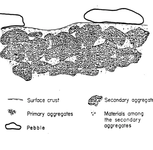
The top layer of the soil is a well developed desert pavement (Fig. 7). The soil particles are cemented together by clay particles, the surface crust forming after the soil has been wetted by rain and dried. This crust is much more mechanically stable than the under-lying soil and makes the desert pavement highly resistant to wind erosion. However, the surface crust can be disturbed by the weight of vehicles or man, exposing highly erodible particles. A soil survey conducted by Leavitt (1974) assessed three sites in the GMX area down to a depth of 152 em. He found the topmost layer to be textured gravelly or cabby sandy loam of low organic content, well to excessively drained with slow run off and rapid permeability (2~-10 inches of
rainfall per hour). The soil is of volcanic origin and was formed from limestone, basalt, quartzite, and rhyolite. Moderate wind and water erosion is evidenced by the low wind hummocks around plants and the shallow stream channels prevalent. The top 15 cm is soft, friable, non-sticky, non-plastic and exhibits a weak fine platy
19 Surface crust
~
Primary aggregates~
Pebble~
Secondary aggregate....
Materials among the secondary aggregatesFig. 7. Soil Structure of the Desert Pavement (after Chepil and Woodruff, 1963)
structure. Rocks and pebbles abound on the surface, with average lengths and heights of 15 mm and 8 mm respectively. They cover about
25% of the surface area.
Tamura (1974) determined the soil particle size distribution and plutonium content of the upper 3 cm soil layer (Table 3). The mean diameter of the desert pavement soil is 70 ~m, if the soil particles with diameters over 2000 ~m ("gravel") are neglected. Chepil (1941) has shown that the gravel particles are generally not erodible and therefore they have been excluded in computing the 'above mean diameter so that the particle size distribution of the desert pavement might be better compared to that of the hummock-trapped particles. This unerodible gravel comprises a large fraction (33%) of the desert
pavement. The soil size distribution obeys the often cited log-normal soil distribution only for the sand sized particles. The surface layer of this soil is available for wind dislodgement and transport.
The soil was radioactive due to the presence of plutonium oxide. 80-90% of the radioactive content of the soil is in this top 3 cm layer, 95% within the top 5 cm. The major transport of radioactive particles within the soil is due to rainfall washing radioactive particles down from the surface. Because americium has a greater solubility than plotonium, it is removed more quickly from the surface layer leaving plutonium as the main component of the wind-erodible surface soil particles. Soil microorganisms are also
responsible for the downward transport of radioactivity (Gilbert and Eberhardt, 1974). The radioactive particulates are less susceptible to erosion as they penetrate deeper into the soil.
Plutonium becomes intimately associated with the soil within a few months after deposition. The movement of radioactive particles is then directly related to soil erosion. The plutonium is not evenly distributed in the soil and "hot" spots are present. No apparent dependence of radioactivity upon the soil particle size has been discovered; therefore, the usual assumption is that the radioactivity is simply proportional to the soil mass (Anspaugh and Phelps, 1974).
Tamura also sampled the soil in a bush wind hummock located within ten feet of his desert pavement sample (Table 4). This soil size distribution differed markedly from that of the desert pavement soil, especially in the conspicuous absence of gravel particles. The median diameter of the soil fraction was 120 ~m, again neglecting gravel. A log-normal distribution fit the sand size distribution. This "blow" sand has a higher concentration of fine sand than the pavement, due to the different natures of the soils. The pavement has developed a platy structure, whereas blow sand is very loose. Thus, the pavement size fractions often represent aggregates formed by finer sizes, while the blow sand fractions represent individual particles. The bush hummocks are more radioactive than the desert pavement. The wind hummocks gave higher surface radioactivity readings (21,000 cpm) than the bare pavement (15,000 cpm) and also
showed a higher activity per unit weight of soil (3100 vs. 2570 cpm/gm). Soil density measurements found the desert pavement soil to
3 have a bulk density of 1.56 g/cm
3 2.22 g/cm .
and a particle density (p ) of P
3 The bulk density of the blew sand was 1.37 g/cm
3
of silica sand particles is 2.65 g/cm3. The particle density was
measured using a non-polar, highly wettable liquid to fill intersticies.
2.6 Bush Hummocks
Bush wind hummocks are mainly associated with creosote bush clumps. The smaller bursage has no discernible hummock, and the occasional IIs ingle" creosote bush has either a noticeably smaller
hummock or none at all. Measurements of 20 creosote clumps found the average hummock height to be 5 cm (Table 2). For these same bushes the following correlations were found:
Correlation Correlation coefficient
Hummock height with shrub height 0.76 Hummock height with shrub diameter 0.66 Shrub height with shrub diameter 0.69
indicating that either: 1) the larger plants are older and have had more time to build a mound, or 2) the larger plants are more efficient at building mounds than the smaller bushes. Probably both mechanisms contribute to the observed correlations.
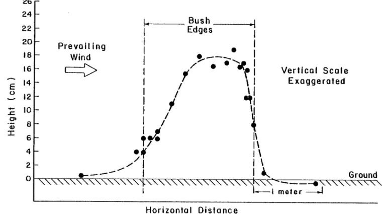
Comparison of the test bush with the 20 bush average is informative:
Maximum Height Average Diameter Mound Height Test bush 0.9 m 2.2 m 18.5 cm Bush average 1.06 m (cr = 0.22 m) 2.07 m (cr
=
0.60 m) 5.0 em (cr=
3.3 em)Figure 8 shows the hummock profile of the test bush. Note that the mound edges coincide with the bush edges. There is some
N lJl Vertical Scale Exaggerated '\.,,~-- - - .:.;e~'\.:""""" \---- 1rn ete r
---J
I~ Bush.1
EdgesI
I
e _-_.
I
/:i' • •it.
I
,
r
l
/
\ I
I
\
I
;
."
/\~
I
/
,
~..:
1\
1/1\
ef
1\
.,;/ I
I \
e_---...
I
.I '-
.
~ Ground Prevoil ing Windc=>
26 24 22 20 18 16 E 14 u 12 ..- 10 ..c 01 Q) 8:c
6 4 2 0 Horizontal Distanceassymmetry in the profile. It is assumed that this is a lltyp ical"
hummock profile.
Dead organic material is prevalent inside the bush. It consists of dead leaves, flowers, fruit, and twigs.
3. EXPERIMENTAL MEASUREMENTS
3.1 Field Instrumentation
The meteorological measurements used in this study were: 1) wind and temperature readings above and below the average shrub height from instruments on meteorological towers near the test bush allowed the flow in the two regimes to be compared, 2) average and turbulent flow velocities close to and inside the test bush were measured by three hot wire anemometers, and 3) the ~vind data necessary to estimate the horizontal erosion flux was obtained from a climatological wind measuring station (SYSTRAC #15).
Two ten meter towers and their associated equipment had previously been established on the western edge of the GMX area at the test
bush site by the Las Vegas Air Resources Laboratory of the National Oceanic and Atmospheric Administration (NOAA). A standard vane and cup anemometer continuously recorded the wind direction and speed
at ten meters. Cup anemometers measured the ten minute mean horizontal wind at five levels (~, 1, 2, 4, and 8 m). A separate cup anemometer at 2 m continuously recorded the wind speed and a 2 m bivane continuously sampled the horizontal and vertical wind fluctuations. All the cup
anemometers were periodically wind tunnel calibrated. Temperatures were measured every ten minutes at five levels. Two levels were below the soil surface at 1 cm and 3 cm. Above ground quartz sensors
in aspirated shields measured the air temperature at ~, 2, and 8 m. A hydrothermograph, supplemented by sling psychrometer observations, provided relative humidity readings. ~~ aneroid barometer recorded the atmospheric pressure. Soil moisture was obtained by averaging
five samples from the upper 0.5 cm soil layer. Each sample was weighed, oven dried, then re-weighed. NOAA personnel performed the data collection and recording tasks.
Three Datametrics SOO-VTP constant resistance-ratio hot wire anemometers measured the mean and turbulent flow in and around the chosen bush. These battery powered instruments operated up to six hours on one charge. Because their lead length was limited to eight feet, the associated electronics were housed in chilled insulated ice chests to keep them at acceptable temperatures. The self-cleaning probes consisted of 0.5 cm long stainless steel filaments. The
manufacturer specifies their accuracy to be within 2%, and their frequency response to be 100 hz. The output voltage response is non-linear and zero drift is possible. The hot wire voltages were recorded by an Incredata digital recorder at a rate of 145 readings per second per anemometer.
The three hot wire probes were suspended from aluminum tubing in either a horizontal or vertical arrangement around the test bush. Generally measurements were made at heights of 96, 45, and 4 cm. These heights were based upon the 90 cm height of the test bush. The 96 cm height was just above the bush, the 45 cm height was half the bush height, and the 4 cm height gave wind speeds close to the ground. A bivane located close to the bush was used to sight a landmark indicating the prevailing wind direction, towards which the hot wire probes were then oriented. The wind direction was also checked after each measurement. Before and after each measurement period the hot wires were covered and the zero velocity voltage was recorded.
29
Climatalogical winds near Frenchman Lake were measured by SYSTRAC station 15, located 3~ km south of the meteorological tower. This permanently sited cup anemometer station was periodically
queried by remote control and in reply gave the ten second wind average at a height of 10 m. This station has operated from August 1969 to August 1976 with only a 15% loss of data. These breakdowns occurred randomly, usually in blocks of days or weeks. The climata-logical data is weighted towards the first two years when the sampling interval was 5 minutes, after which it changed to 15 minutes.
Besides the hot wire anemometer data, the digital recorder also recorded the output of a Meteorology Research Inc. Model 1550B
nephelometer. This instrument measures the backscattered light
from particulates in a control volume, thereby indicating the particu-late loading of the air. The nephelometer sampled the air 10 cm
above the ground at a location three meters from the test bush. It was designed to provide 10% accuracy and withstand a 0°-130° F temperature range. The inlet sampling tube introduced a time delay of 0.8 sec, the time constant of the instrument being 2 sec. Although only qualitative measurements of the atmospheric dust content were needed, nevertheless the nephelometer was calibrated, using Freon gas as a backscatter coefficient reference.
3.2 Hot Wire Anemometer Data 4\nalysis
The hot wire anemometers were individually calibrated in a wind tunnel by comparing pitot tube velocity calculations with output voltages measured by a digital voltmeter. This voltmeter also
in the field. A third order polynomial was fit to each calibration curve and used to convert each recorded anemometer voltage into a corresponding velocity.
The "velocity" measured by a hot wire anemometer is actually a "mass velocity" L e. the product of air density times velocity. Therefore all calculated velocitites, measured both in the field and in the wind tunnel, had to be corrected for density to obtain the true velocity. Air temperature and pressure data were thus needed in both cases. This presented difficulties for the field data, since velocity measurements were made at a 4 cm height while the lowest air temperature sensor on the meteorological tower was at 50 cm. To overcome this probleo, a constant temperature differential between the two layers was assumed. This temperature difference was estimated to be 4°C from comparisons of the measured temperature profiles to temperature profile formulas developed by Malurkar and Ramdas (1931). Because the field measurements were all taken during the afternoon on sunny days, the air temperature on a given day was relatively constant (2°C maximum range). Since the density depends upon the absolute temperature, errors from this source were negligible compared to other errors in the velocity measurements,. e.g. a IOC temperature error would give a velocity error of only 0.3%.
In the field the hot wire anemometers were compared both to themselves and to the cup anemometers on the meteorological tower. For intercomparison of the hot wires they were placed a foot apart at a 2 m height in an "isolated" spot, Le. one far removed from nearby bushes. The flow past each of the anemometers should be the same. An 18.3 minute test (150,000 values per hot wire anemometer)
31
gave velocities of 3.96, 4.00, and 4.01 m/sec for the three anemometers, showing agreement within 1%. The standard deviations obtained
agreed within 5%. To compare the hot wire anemometers with the tower cup anemometers, a 40 minute test was made with a hot wire anemometer located a foot to the side of both the 1 m and 2 m tower cup anemometers. The average ratios between the four ten minute mean cup velocities
and the corresponding ten minute mean hot wire velocities were 1.144 (cr
=
0.017) at 1 m and 1.139 (cr=
0.029) at 2 m. The ratios agreed to a surprising degree for both heights. The source of the discrepancy between the hot wire and cup anemometer velocities is cup anemometer "overspeeding", a well-known effect resulting from the cup characteristically accelerating faster in gusty winds than it decelerates. The magnitude of this overspeeding error was consistent with the results of an intensive investigation of cup overspeeding errors made by Izumi and Barad (1970). They found the overspeeding to average 16% of the wind speed, but noted that tower influences could account for as much as 5% of this and that stability also influences the overspeeding. They suggested that the best estimate of overspeeding error was about 10%. The cupanemometer speeds obtained were corrected for overspeeding by multi-plying them by a factbr of 0.876, the average of the above two
ratios. Using this ratio for all heights is justified by the agreement between the 1 m and 2 m ratios and by Izumi and Barad's conclusion that no strong relationship existed between overspeeding error and anemometer height.
One major source of error in hot wire anemometer measurements can be zero drift. To minimize this the anemometers were covered
before and after each measurement period and the zero velocity voltage was recorded. Because the measurement periods were relatively
short (~30 minutes), this was done often enough that the change in
zero velocity voltage was generally small (average drift ~ 0.08 mv/min). A one millivolt error gives a velocity error of 0.45% at a velocity of 3 m/sec. In the data reduction the zero velocity voltage used to calculate the velocity from the recorded voltage was presumed to be a linear interpolation of the zero velocity voltages measured before and after the measurement period. Unfortunately there were two periods where an end zero velocity voltage was not obtained. Taking a "worst case" zero drift for the longer of the two periods, a maximum average velocity error of 1.2% was calculated. This is small enough to be ignored.
Hot wire anemometers respond not to wind flow in one direction only but to the flow in a plane perpendicular to the wire. Thus a horizontally oriented hot wire will also respond to vertical flow, but not to horizontal flow parallel to the wire. Practical consider-ations of placing a probe very close to the ground forced the use of a horizontal orientation for the hot wires. Any change between the mean wind direction and the plane normal to the hot wire would result in the measured velocity decreasing according to the cosine of the angle, a relationship verified during the wind tunnel cali-bration. I f the angle increased beyond 15° the presence of the probe posts would further decrease the measured wind velocity. It was therefore important that the wind direction remain essentially constant. Fortunately the wind direction during the field measurements was remarkably steady. The nearby bivane inked record was checked
33
for wind direction before, during, and after each measurement. Two measurement periods which showed variations greater than ten degrees were discarded. Such a ten degree variation would give an error of
2% according to the cosine law.
With the hot wire element horizontally oriented, any mean vertical wind would give a measured velocity greater than the actual horizontal wind. Although there is definitely vertical flow due to the bush, estimates using the continuity equation showed it to be generally negligible (See Appendix A).
Because the hot wires also respond to turbulent fluctuations in the vertical direction, turbulence will cause the measured velocity to be greater than the actual horizontal velocity. This effect was estimated and found to be negligible except close to the ground behind the bush where turbulent intensities of up to 0.7 are found. Such high turbulence levels would produce an estimated error of 7% (See Appendix A). Since a hot wire anemometer is unable to distinguish flow direction, such large turbulent intensities raised the possibility that intermittent reverse flow might have occurred. However the velocity frequency distributions of these cases were essentially Gaussian, which would not be expected if reverse flow was significant.
Surface friction leads to the formation of a boundary layer below the geostrophic wind. In this boundary layer mom€ntum is transferred downward by turbulent wind shear and bouyant motions to the surface layer. The surface layer is defined as that region where the fluxes of momentum, heat, and moisture are independent of height, to a first approximation. The height of this layer can extend from 10-50 m. When considering flow over a vegetated surface the momentum flux is constant only in the horizontally homogeneous flow above the wake interaction region. Below this height horizontal inhomogeneities produce stress variations with height.
The ground and obstacles above it, e.g. vegetation, exert a drag on the air flow called the total surface stress (,). The
o surface friction velocity is defined as:
(4-1)
where p
=
air density. In the surface layer the vertical momentum flux (F ) is constant, equal and opposite to the shear:m
where , shear stress
F = -, =
+
P uwm (4-2)
u
=
fluctua:ing horizontal velocity w=
fluctuating vertical velocity.Momentum transfer is often described by semi-empirical relationships. One method, analogous to molecular transport in viscous flow, uses
the velocity gradient and an eddy turbulent transfer coefficient (K ):
m
35
F
=
-pK
au
m m az
A second method uses a transfer coefficient in integrated form:
(4-3)
F m 2=
-p Cd U . (4-4) Both Kmand Cd are functions of height. The "meteorological" surface drag coefficient (Cd) used here is one-half the value of the "aero-dynamic" surface drag coefficient (C
da):
C
=
kC=
(u*\
2d zda
u)
.
The logarithmic wind law is known to adequately describe the velocity profile in the surface layer under neutral conditions:
u*
u
=
k
In .;-owhere k
=
von Karman constantz
=
characteristic length of surface roughness. o(4-5)
(4-6)
u*
is a useful scaling velocity for the surface layer. z is often oused to scale the eddies responsible for the drag on a rough surface. The logarithmic wind profile can be derived either: 1) by assuming a constant stress, neutral conditions, and mixing length theory, or 2) more generally, i.e. with fewer restrictions, by asymptotic matching of a law of the wall with a velocity deficit law of the outer flow. The logarithmic wind profile can also be valid for heights above the surface layer, up to 100 m or more.
The von Karman constant (k) has traditionally been given a value of 0.4, based upon laboratory experiments. Experiments in the
atmosphere, with higher Reynolds numbers than are typical of laboratory flows, show a large scatter. The most extensive experiments to
date, conducted in a Kansas field, indicated k : 0.35 (Businger et al., 1971). This value has been accepted by many micrometeorologists
because it agrees closely with the k : 0.33 value Tennekes (1968) deduced by extrapolating wind tunnel measurements to very large Reynolds numbers. Some disagreement continues, however, as Pruitt et al. (1973) found k values between 0.39 and 0.44. The von Karman constant used in this thesis was the traditional 0.4 value.
In dealing with flow over vegetation, the height where the mean wind vanishes according to the logarithmic wind profile may not be the ground itself, but some height above the ground which acts as a new surface with respect to the wind, the zero plane displacement height (D ). Eq. (4-6) then becomes:
o
where Z
=
characteristic roughness length above vegetation.o
(4-7)
The neutral case requires that there is no heat flux from the surface to the atmosphere. In the more usual diabatic case, heat flux is present. The associated bouyancy forces may playa significant role in modifying the surface layer wind profile. The Richardson number (Ri) is often used as a measure of stability:
(r
+
l'!.)
=
bouyancy transfer of momentum _ ~ dZRi mechanical transfer of momentum - T (aU/3z)Z
where g : gravitational acceleration
r
=
adiabatic lapse rate.37
Another stability parameter, the scaling length L, was introduced by Obukhov (1946) using similarity arguments. L is usually called the Monin-Obukhov length:
(4-9)
where 8
=
fluctuating temperature. L is used to define theMonin-Obukhov dimensionless height, ~
=
z/L. The advantage of this represen-tation is that L is approximately constant in the surface layer,whereas the Richardson number is not. In diabatic conditions Eqs. (4-6) and (4-7) must be modified, as will be described later.
Whether the roughness elements are densely spaced or not, at
some height their wakes interact and are integrated into a horizontally homogeneous flow. The outer flow above the wake interaction region is the constant stress region described by Eq. (4-7) for neutral condi-tions. The existence of this constant stress layer above the vegetation has been well documented in both wind tunnel work (O'Laughlin and
Annambhotla, 1969; Plate and Quraishi, 1965; Sadeh ~ al., 1971) and in field experiments (Kutzbach, 1961; Thom, 1971). The constants in Eq. (4-7) are determined by the combined effects of single roughness elements. An individual roughness element is generally characterized by a height (H), a diameter (D), and a porosity (¢).
When considering uniformly scattered roughness elements the specific area, i.e. the ground area per roughness element (S), is an important parameter. 11any empirical formulae have attempted to relate Z and
o D to H, D, and S. For example, Lettau (1969) suggested:
o
z
=
~ HD/s .This formula has been found to-be most useful when the roughness elements are somewhat isolated. Other proposed formulae are more adequate when the individual roughness elements are so close that
they have lost their identity, i.e for· canopy flow. Empirical formulae for D have also been proposed for such cases. Seginer (1974)
o
references much of this work.
In the upper flow regime the mean and turbulent velocities depend solely upon the height above D and the shear stress, not the parameters
o
of the roughness elements that produce this shear stress. Morris (1955) has noted that the distance from the ground to this upper flow regime depends primarily on the frequency and size of the vortices formed by the roughness elements. Woodruff ~ al. (1963) found the height of the wake interaction region for actual and model windbreaks to extend to 2.0 Hand 1.8 H respectively for downwind distances of 20 H. O'Loughlin and Annambhotla (1969) found wake depths of H to 1~ H for flow over roughness elements, while Sadeh et al. (1971) found depths of 1.7 H. Flow experL~ents over two-dimensional solid windbreaks, where the vertical flow is of necessity much greater than for porous ones, found a wake interaction region up to 2-4H (Good and Joubert, 1968). Based upon the average bush height of 1 m, the height of the GMX wake region was estimated to be less than 2 m. Therefore, velocities at and above 2 m were considered to represent the constant stress outer layer.
The preceeding arguments have concerned the horizontally
homogenous flow above the wake interaction layer. Below this height the effect of individual roughness elements must be considered. Vegetation interacts with the mean flow wind by 1) extracting the
39
momentum required by the aerodynamic drag of plant parts, 2) converting mean kinetic energy into turbulent kinetic energy in the wake formed behind an obstruction, and 3) breaking down large scale turbulent motions into smaller scale motions in the wake region.
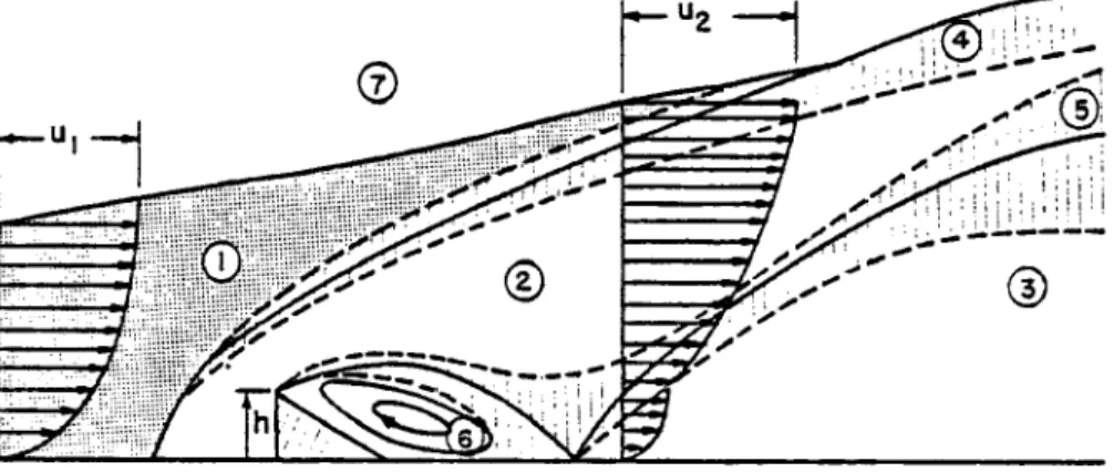
The flow past an individual two-dimensional roughness element, e.g., a windbreak, will be described first. The incident flow is distorted, producing a pressure differential across the element, and separation bubbles ahead of and behind solid obstacles. A wake or shear zone extends above the near separation zone. Intense shear transfers mean kinetic energy into turbulent energy, resulting in increased mixing. The greatest velocity reductions occur in region~ of greatest mixing. The velocity profile continually adjusts until the excess mixing becomes negligible. Downstream of the separation zone, a new boundary layer flow develops in equilibrium with the underlying surface (Fig. 9). This internal boundary layer grows slowly downstream, eventually displacing the wake region. Stream-lines on the upwind side start to rise before reaching the obstacle, reach a maximum at a point beyond the obstacle, and then slowly drop. The drag exerted on the airflow reduces the wind velocity, as
indicated by the upward rise of the streamlines. The surface stress is also reduced (Fig. 9) • The sheltered zone has been estimated to extend from 5 H windward to 30 H leeward (van Eimern
!:!.
al., , 1964). The wind reduction at lower heights is balanced by a corresponding windspeed increase at upper levels, as required by the law of continuity. For porous obstacles the flow features are qualitatively similar, except that the lesser pressure differential across the element
T ITOI , r - -...
'\~:!~:~:----::::::o---o
'1-- _p-p
_ _t 0
Pt
~--Fig. 9. Airflow Regions Behind a Windbreak (after Plate and Lin. 1965 and Seginer and Sagi. 1972)
41
changes are less abrupt and the turbulence is less intense. The decreased mixing allows the wind reduction zone to extend further downwind. At the front and rear of a porous screen, both the pressure and velocity are approximately constant with height. The air flowing through the screen provides the leak which reduces the pressure
differential across the obstacle. This pressure drop is proportional to the velocity squared, in agreement with the drag force (F
d) equation:
(4-11)
where the drag coefficient of the obstacle (Cd) is a function of porosity.
For porous plates i~ a wind tunnel, Castro (1971) found that the vortex street and reversed flow recirculation region, two
character-istics associated with flow behind solid objects, both disappeared when the plate porosity increased beyond 30%. Bleed air entraining into the shear layers prevented them frcm interacting. The effective
porosity of the creosote bushes will be found to be 70-80%. Obstacles of such large porosity can be considered to be lattices whose
separate elements are of sufficiently small width that they have negligible individual effect on the flow, but which together form a uniform sheet of resistance. The main effect of such a structure is to produce a drop in the total pressure along any streamline passing through it. A summary of relevant formulae has been given by Graham (1976).
The windbreak discussed above has been assumed to be two-dimen-sional. Estimates of the length to height ratio required to meet
this assumption have ranged from 12 to 24. A ratio of two reduces the protective effect by one-half (Bleck and Trienes, cited by van Eimern ~ al., 1964). Flow past a three-dimensional object involves additional turbulent mechanisms. As the flow passes the roughness elements, the wake vortices transfer vorticity from the mean shear to the flow direction itself. The shear is greater than that of two-dimensional flow and more turbulent kinetic energy is generated. Initially this turbulence is scaled to the dimensions of the roughness element, but further downwind the distance from the surface becomes the scaling length just as it was far upstream. The lateral velocity deficit region grows linearly with distance downstream and soon
becomes Gaussian (Meroney, 1968).
Plants create disturbances, whose individual effect is soon dissipated but whose aggregate effect determines the intensity and nature of the turbulence. In the region below bush height the time averaged flow is three-dimensional, and a one-dimensional model can be only partially adequate. Two types of flow have been
observed, isolated roughness flow and canopy flow. The latter can be further divided into wake interference flow and skimming flow.
The "isolated roughness" type of flow occurs when individual roughness elements are far enough apart that the wake and vortex of each element have completely developed and dissipated before the next element is reached. In such a flow, Eq. (4-7) is valid above the roughness element height. Z is greater than it would be for
o
the surface alone, since it is a measure of the surface drag and the projections considerably increase this drag.
43
"1;-J'ake interference" flow occurs when the roughness elements are close enough that the wake and vortex of an element interferes with the flow at following elements. When the roughness elements are so close that stable vortices or pockets of "dead" air are formed, the flow is called "skimming" flow. In both cases the roughness
elements are packed so closely that a new uniform surface, the canopy, is formed by their tops, and the surface layer is displaced upward by the displacement height D
o Eq. (4-7) is valid above the canopy height. Below this height a complicated, but comparatively weak, canopy flow exists. It is usually treated as a one-dimensional flow, and an exponential wind law has often been observed (Inoue, 1963; Cionco, 1972):
Ua exp [a (z/H - l)J
where a is an empirical constant.
(4-12)
The main difference between the flow inside vegetation and above it is that in the former case momentum can be absorbed directly by the vegetation and the equation of motion becomes:
a(uw)
=
az
1
ap
n
2- - ....- - cd(-S)p
ax
U (4-13)where
P
= mean pressure andn
= foliage area per unit volume. Both cd andn
are usually complicated functions of height, and cd is also somewhat dependent upon wind speed.Three flow regimes are distinguishable in well-developed canopy flow:
1) in the upper part of the canopy the pressure term is negligible;
2) in the middle of the canopy the divergence of the momentum flux is negligible, especially for a dense canopy; and 3) very close to the surface a(~)/az
=
0 and the windprofile is logarithmic. The height of this region depends upon the roughness element spacing.
Seginer (1975) has shown that turbulent mixing dominates bouyant effects close to a windbreak. Stability effects can be significant for downwind distances beyond 3 H, reducing the sheltering effect by approximately 10%. Uchijima and Wright (1964) found no large thermal effects in a corn crop canopy study covering a wide range of thermal stabilities.
In the following analysis of the flow in and above the desert chaparral of the G}~ region, the following conclusions will be reached. The creosote bushes are widely spaced and aerodynamically very
porous. They act as individual roughness elements, each producing a wake that is essentially dissipated by the time it reaches the downwind bushes. The flow is closest to the "isolated roughness" flow, not the "canopy" flow produced by more closely spaced elements. The wake region of a bush is similar to that of a two-dimensional windbreak, with an internal boundary layer developing downstre~~. These wakes combine and merge vertically within twice the bush height. A horizontally homogeneous, constant stress region exists above this wake interaction region. Due to the close and regular spacing of the branches, the flow within an individual bush has properties similar to that of flow through a canopy, although the flow has not had time to become well-developed.
5 • AIRFLOW MEASUREMENTS
5.1 Flow Above the Vegetation
The airflow above the shrubs was investigated because 1) it provided clues to the type of flow below shrub height and 2) the results were used to estimate the partitioning of the total drag between the bush and the ground, an important factor in assessing the ability of vegetation to control wind erosion.
A great deal of effort has gone into developing relations
between the momentum flux and the wind profile under unstable conditions. Barad (1964) gave a historical account of 30 years of work measuring surface stress in the surface layer. Under neutral conditions the surface stress can be easily determined from the logarithmic velocity profile, but diabatic conditions require consideration of bouyancy effects. The GMX velocity profiles were obtained under unstable daytime conditions. Therefore a diabatic flux relationship was used to obtain the stress above the vegetation.
In the most extensive measurements to date, Businger et al. (1971) related the dimensionless wind gradient to 1;. Paulson (1970) integrated this relationship, giving:
where ~ :: diabatic velocity profile correction
:: 2 1n [(1+s)/2J + 1n [(1+s2)/2J - 2 tan-1 s + rr/2
1
S :: (1 - 15 1;)"'.
(5-1)
For measurements over vegetation, the zero plane displacement must be added to the above equation:
u
=
-
~)
(5-2) where now ~=
(z - D )/L.o
Eq. (5-2) was employed to obtain "best fit" values of Z o and D for the GMX area from 89 concurrent wind and temperature profiles
o
measured at the meteorological towers. Since the region of interest was the constant stress layer above the wake interaction region, only the winds at 2, 4, and 8 m were used. The long upwind fetch insured that the 8 m velocity was well within the constant stress region.
The Richardson number at 4 m was computed using wind and temperature gradients determined by fitting a quadratic of (In z) to the wind and temperature profiles. The Monin-Obukhov length was then calculated using Businger et al.'s (1971) empirical relationship:
0.74 C (1 - 15
~)~
Ri
=
~(l - 9 1;) 2
Knowing L, ~ could be calculated for each of the wind profiles.
(5-3)
Munroe and Oke (1973) found no statistically significant relation between either Z or D and wind speed, contradicting the results
o 0
of other investigations. They attributed the Z and D variations
o 0
found by others to inadequate diabatic corrections and streamlining effects. Accordingly, Z and D in the GHX area were assumed to
o 0
remain constant under all wind conditions and a U* for each indi-vidual profile determined from a least square fit. The sum of the
squared difference between each estimated and measured velocity was computed, and the values which gave the minimum squared velocity
error were Z = 2.7 cm and D
o 0
percentage was 0.52%.
47
8 cm. The average velocity error
To determine whether the Z and D values calculated in this
o 0
manner were a function of stability, the wind profiles were separated into stability classes and the above process repeated. The calculated Z and D values exhibited no definite trend with stability, therefore
o 0
the diabatic velocity profile correction used above introduced no systematic error.
It is interesting to compare these results to those which would have been obtained by assuming neutral conditions. Using the above method with no diabatic correction gave Z = 0.73 cm and D = 25 cm,
o 0
the average velocity error percentage being 1.1%. As might be expected, when separated into stability classes the calculated Z
o and D values depended strongly on stability. The diabatic correction
o
does not introduce an additional degree of freedom, so the decrease in the velocity error obtained by using it is significant.
In simultaneously determining Z and D , there was a strong
o 0
interaction between the two and the minimum was rather broad. This should not affect the U* values calculated for each profile.
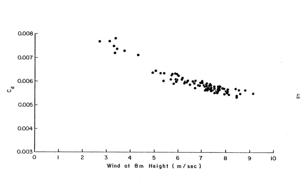
Figure 10 gives as a function of wind speed the 8 m meteorolog-ical drag coefficient, C
d(8 m) = u*/U(8 m). The 8 m drag coefficient decreases for stronger winds, in agreement wit~ :ield studies of
a windbreak (Seginer, 1975) and of a crop canopy (Uchijima and
Wright, 1964). Since the total drag is the sum of the form (pressure) drag and skin friction, the total drag should not increase in
propor-tion to the velocity squared, so it is not unexpected that the drag coefficient varies. The total drag results mainly from bush drag,
••••
"0 U0.007
0.006
•• •
•
•
",
.
• ·.t ".
'!..
".1-:(
~..
I ·
6t .p. 000.005
0.004
109
83
4
5
6
7
Wind at 8m Height (m/sec)