Investigating Adaptive Trajectories to Explore Water Plumes on Icy Moons

(1)

IN

DEGREE PROJECT ENGINEERING PHYSICS, SECOND CYCLE, 30 CREDITS

,

Investigating Adaptive Trajectories

to Explore Water Plumes on Icy

Moons

MARCUS ACKLAND

KTH ROYAL INSTITUTE OF TECHNOLOGY

(2)

(3)

Investigating Adaptive

Trajectories to Explore Water

Plumes on Icy Moons

MARCUS ACKLAND

Master in Aerospace Engineering Date: September 17, 2018

Supervisor: Nickolay Ivchenko (KTH), Uland Wong (NASA), Michael Dille (NASA)

Examiner: Tomas Karlsson

Swedish title: Undersökning av adaptiva omloppsbanor för utforskning utav vattenplymer på ismånar

(4)

(5)

iii

Abstract

This thesis investigates different means of introducing autonomy into designing spacecraft trajectories by surveying four different adaptive trajectories. This is done using established algorithms within path planning and robotics, implementing trajectories based on splines and greedy algorithms. The survey is based on real planetary data let-ting the spacecraft fly through the water plumes on Enceladus. These plumes are constructed using analytical models of the water plumes that have been fitted to measurements made by Cassini during flybys over the last decade. A mission designed to probe these plumes at an altitude as low as 5 km is studied as a test scenario for the adaptive tra-jectories. It is found that the adaptive trajectories increase the science return at lower altitudes, both in exploring the terrain and sampling the plume material.

(6)

iv

Sammanfattning

Uppsatsen undersöker sätt att inkludera autonomi i designen av om-loppsbanor för framtida rymduppdrag. Totalt undersöks fyra olika ad-aptiva omloppsbanor som baseras på etablerade algoritmer inom ro-botik för att självständigt nagivera sin omgivning. Omloppsbanorna består av två kategorier: algoritmer baserade på splines och giriga al-goritmer. Undersökningen utförs genom att flyga igenom vattenply-merna på Enceladus för att förankra den i en verklig miljö baserad på planetär data. Dessa plymer är konstruerade med en analytisk modell för densitetsfältet som är baserad på mätningar av Cassini det senaste årtiondet. Omloppsbanorna testas i ett exempeluppdrag där plymerna undersöks på en altitud ned till 5 km. Resultaten från undersökingen visar att de adaptiva omloppsbanorna returnerar en högre avkastning vid lägre altituder på viktiga mått som uppsamlad densitet och utfors-kad area.

(7)

v

Acknowledgement

All work for this thesis has been carried out at the Intelligent Robotics Group at NASA Ames Research Center under the ICICLES project supported by NASA’s COLDtech program. I am extremely grateful to my mentors Dr. Uland Wong and Dr. Michael Dille for their valu-able input and guidance during my internship. My participation in this program would have been impossible without the Swedish Na-tional Space Agency, the agency that nominated me to NASA.

I also want to thank my advisor at KTH, Dr. Nickolay Ivchenko for his help throughout writing this thesis. Dr. Lorenz Roth who let me work on his research on Europa and the water plumes detected there. This introduced me to the subject of water plumes and without his support I would not have had this opportunity.

Lastly I want to thank my family for all their support, not only enabling me to write my Master’s thesis at NASA but during my entire time at university. This is true especially for Izze, to whom this thesis is dedicated.

(8)

Chapter 1 Introduction

When Cassini-Huygens was launched in 1997, it was originally planned to be a four year mission. Expectations of what might be discovered were likely high, but it is safe to say that the results far surpassed what could have been anticipated. When the mission ended with Cassini crashing into Saturn in 2017, it did so after nearly two decades of ex-ploring the Saturnian system and left behind a legacy of extraordi-nary results. From the Huygens probe’s discovery of seas of liquid methane on Titan to Cassini imaging exotic storms on Saturn. One of the most significant discoveries is the giant water plume on Enceladus, Saturn’s 6th largest moon [15]. The discoveries made by Cassini has el-evated Enceladus alongside Mars and Jupiter’s moon Europa, another icy moon, as one of the most promising locations of finding life in the solar system.

Despite the huge success of the mission, the instruments on Cassini were not designed to detect life and the primary objective was never to investigate the plume on Enceladus. There are still questions left to be answered, mainly concerning if the moon harbors life or not. This has generated support in the scientific community for a follow up mission going back to Enceladus with proper instrumentation and the primary objective of detecting life [12]. This has not been done since Viking was sent to Mars, over four decades ago.

The main goal of this thesis is to survey different means of incor-porating autonomy in designing trajectories and have the spacecraft adapt to the environment it is flying through. A mission going back to Enceladus would likely orbit Saturn which leads to a limited number of flybys, the adaptive trajectories proposed in here are designed to

(12)

2 CHAPTER 1. INTRODUCTION

increase the science return of every flyby.

The work of this thesis has been done at the Intelligent Robotics Group at the NASA Ames Research Center in Mountain View, Califor-nia.

1.1 Motivation

With the retirement of the ISS just a few years away, NASA has de-cided to shift their focus toward interplanetary space missions [13]. With this focus come a necessity to develop autonomous capabilities which enables spacecraft that cannot communicate with Earth to work independently of input from mission control. There has been a tremen-dous wave of innovation in automation in other industries such as self-driving cars and UAVs but so far we have not seen this leap in space exploration.

NASA wants to investigate areas where autonomy can be intro-duced and this thesis aims to survey ways of including autonomy in designing trajectories. The plume sources on Enceladus offer an in-teresting backdrop to perform this study for a couple of reasons. The individual jet sources have been studied thoroughly but there are still some questions left to be answered regarding their exact location and behaviour. The motivation behind this survey is to study a space-craft probing the plume at a much lower altitude than previously at-tempted. For a spacecraft flying at lower altitudes, autonomy will be helpful since the exact location of the sources is not fully known. If the spacecraft is autonomous, the planning of the orbit does not have to be as exact in pinpointing the plume sources. Secondly, the spacecraft will travel very quickly through the plume and utilizing autonomy to steer the trajectory should increase the science return of a Cassini-like mission.

(13)

CHAPTER 1. INTRODUCTION 3

1.2 Problem statement

The problem statement this thesis aims to answer is:

• How to utilize autonomous capabilities to increase the science re-turn of each flyby, and by which metrics should these trajectories be evaluated?

1.3 Contribution

The contributions of this thesis are:

• Surveyed adaptive trajectories: looking at existing, simple al-gorithms and how they can be used to introduce autonomy in spacecraft trajectory design.

• Created a framework to simulate adaptive trajectories.

• Conceived an archetype mission to explore plumes. This will enable future missions based on real planetary data.

1.4 Limitations

Ideally this thesis would not only investigate different ways of flying over the terrain but also design an algorithm that can outperform tra-ditional algorithms that were not designed with this endgoal in mind. Because of time constraints this has not been looked at but will hope-fully be an area of interest for future interns at NASA.

Another limitation is the generality of the study. The scene that has been studied, the south pole of Enceladus, is very biased and al-gorithms that are successful in this survey might perform worse in another setting.

Except for basic constraints, the actual kinematics of a spacecraft are not used when considering if the trajectories are possible to per-form or not.

(14)

4 CHAPTER 1. INTRODUCTION

1.5 Outline

The outline of this thesis is as follows: Chapter 2 introduces the nec-essary background behind designing the adaptive trajectories and the autonomous capabilities for the spacecraft. It also sets into context the discoveries of Cassini to understand the value of revisiting Enceladus and what environment the spacecraft would find itself in. Chapter 3 discusses the plume model used to create the environment of water plumes as they exist on Enceladus. It also describes how each trajec-tory was designed and how the plume model and trajectories were represented in the simulation. Chapter 4 will present the results of the survey, and Chapter 5 will discuss these result and compare the differ-ent trajectories with each other.

(15)

Chapter 2 Background

In this section Saturn’s moon Enceladus, which is used as an environ-ment for the survey, is presented together with the discoveries made by Cassini during the past two decades. Cassini is the most recent mission to have visited Saturn and Enceladus so the discoveries and lessons learned from that mission is crucial for any future planning. After that, the necessary background for designing the trajectories an-alyzed in this thesis is presented.

Figure 2.1: Enceladus. Source: NASA-JPL

(16)

6 CHAPTER 2. BACKGROUND

2.1 Enceladus

Enceladus was discovered in 1789 by William Herschel and before Cassini little was known about the moon [9]. Images sent back by Voyager in the 1980s revealed a small body with a remarkably reflec-tive surface, the brightest in the solar system. Enceladus was initially thought to be located outside the habitable zone but during the first flyby of the moon, Cassini’s magnetometer picked up a disturbance and it was decided to further investigate the moon. What they found was an active moon with a global subsurface ocean. Since the first discovery of cryovolcanic activiy in 2006, subsequent flybys have con-firmed the existence of a global ocean underneath the icy crust and hy-drothermal vents similar to the ones on Earth. This makes Enceladus one of the most likely locations of finding life in our solar system. Fur-thermore, what makes Encleadus an attractive target for a mission is that the plume sources offer a unique opportunity of making in-situ measurements of the ocean without having to drill through the sur-face or crashing into it like other missions such as NASA’s InSight or LCROSS.

2.1.1 Cryovolcanic activity

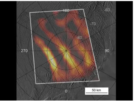
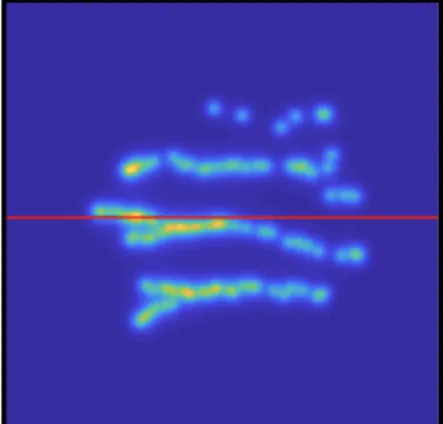
The plume on the south polar terrain of Enceladus has been shown to be made up of individual jets of water vapour and icy particles [6, 15]. On the south pole, four linear fractures dubbed the ’tiger stripes’ are located. These features are named Alexandria, Cairo, Baghdad, and Damascus. It is from these fractures that the water geysers origi-nate from. These features have also shown to emit a surprisingly large amount of heat. These stripes together with the heat emitted is shown in Fig 2.2. Years before Cassini was able to confirm the existence of volcanic activity, it was hypothesized to exist. It was believed that vol-canic activity was the source of the E ring of Saturn, similar to the ring formation around Jupiter at Io’s orbit [14].

Despite the plume looking like one giant cloud from afar, it has been found to be made up of smaller individual sources that all con-nect to the same global ocean beneath the surface. It was first believed that the plume originated from 8 different sources [21]. A 6.5 year sur-vey of Cassini images of the south polar terrain have since revealed 98 separate jets erupting from the tiger stripes to form the giant plume

(17)

CHAPTER 2. BACKGROUND 7

Figure 2.2: Heat emitted from the Tiger Stripes which are

150km long fractures on Enceladus’ south pole. Source:

NASA/JPL/GSFC/SwRI/SSI

[17]. Spitale et al. [22] have proposed the plumes being a continuous curtain of jets instead of discretized sources but this has since been disregarded [16].

While everything is not yet fully understood about the nature of these individual jet sources, it is clear that they vary in strength over time [20, 25]. This does not necessarily mean that individual sources are turning on and off completely but the strength of each source does vary. Most successful models to date have managed to capture this phenomenon by only having some of the sources active when trying to fit their results to data from Cassini flybys [20]. This is believed to be a result of tidal stresses on the surface of Enceladus. As the moon orbits around Saturn, the gravitational force of the planet exercises a varying amount of force that narrows or widen the sources [7, 17].

2.1.2 Indications of life

The ocean beneath Enceladus was first thought to be a regional sub-surface sea of water. However when studying the librations of the fractures on the surface, it became clear that the model of the moon required a global subsurface ocean that completely separates the icy

(18)

crust from the rocky core [1]. Hydrothermal activity has been con-firmed to take place at the bottom of the subsurface ocean [8]. Af-ter Cassini’s Cosmic Dust Analyzer (CDA) detected sodium-salt-rich grains in the plume material, these particles had to have been in con-tact with the rocky core. For them to be transported to the surface high temperatures, near the boiling point, are necessary which require hydrothermal vents at the bottom of the ocean. These appear on the bottom of the ocean here on Earth as well and enable microorganisms to live in areas that have never seen sunlight, a strong indication that they are able to support life on Enceladus just like they do on Earth [8]. In 2017 Waite et al. [26] reported that an abundance of hydrogen had been detected in the plume material. This could have important implications for the potential of detecting organic life on Enceladus as it signals a thermodynamic disequillibrium that favours the formation of methane from CO2 in Enceladus’ ocean.

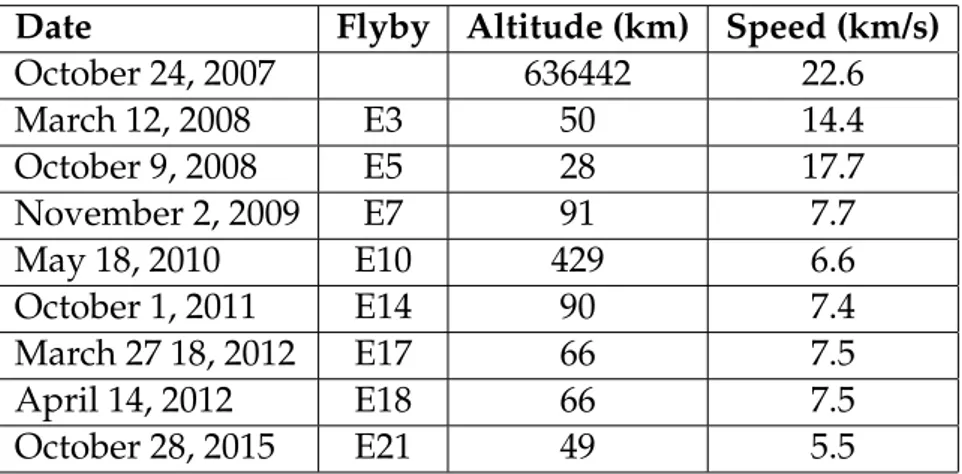
2.1.3 Cassini flybys

Since the first flyby of Enceladus and the discovery of an active moon, the mission flight plan was changed to include more flybys of Ence-ladus and to investigate the plume phenomenon in particular. In total 23 flybys of Enceladus have been made, a significant increase from the three that was initially planned. A clear indication of the importance of Enceladus and the desire to investigate its potential of harbouring life. Seven of these were directly through the plume of Enceladus, listed in table 2.1. As the mission went on, the altitude was lowered to try to learn more about the plume and get more accurate measurements of the plume composition. The closest one was performed at an altitude of 49 km in October 2015. These flybys have generated valuable sci-ence and provided data that is still being studied today. The three key questions the Cassini team wanted to answer in the dive through the plume were:

1. Confirm presence of molecular hydrogen (H2)

2. Better understand the chemistry of material in the plume 3. Determine the nature of the plume sources

(19)

CHAPTER 2. BACKGROUND 9

One significant flaw, however, is that the instruments on Cassini were never designed specifically to detect life or analyzing the material of Enceladus’ plumes.

Table 2.1: List of Cassini flybys of Enceladus’ plume

Date Flyby Altitude (km) Speed (km/s)

October 24, 2007 636442 22.6 March 12, 2008 E3 50 14.4 October 9, 2008 E5 28 17.7 November 2, 2009 E7 91 7.7 May 18, 2010 E10 429 6.6 October 1, 2011 E14 90 7.4 March 27 18, 2012 E17 66 7.5 April 14, 2012 E18 66 7.5 October 28, 2015 E21 49 5.5

2.1.4 Plans for future missions to icy moons

This section is meant to highlight different means of exploring water plumes and what missions are being proposed. Some missions are us-ing flybys while others propose usus-ing landers directly. After the suc-cess of Cassini and with the limitation of its instruments in mind, there is support for a new mission to directly explore the moon. One pro-posed mission is the Enceladus Life Finder (ELF) to assess the habit-ability of the subsurface ocean. ELF would orbit Saturn with the objec-tive of performing multiple flybys through the plumes [12]. Another idea is a lander that would catch the plume particles falling back to the surface [18].

In 2014 scientists studying Hubble Telescope Data found signs of plume activity on Jupiter’s moon Europa similar to Enceladus [19]. This is also an icy moon and given the similar plume phenomenon, there are a lot of parallels to missions planned for Europa. One such mission is the Europa Lander that would be a follow-on mission to Europa Clipper mission and would be targeted for launch in 2024 [5]. One of the objectives of this mission would be to confirm the water plumes on Europa.

(20)

2.2 Trajectory Planning

The planning of a trajectory can be looked at from two criteria: feasi-bility and optimality. In [10], LaValle states that feasifeasi-bility is a matter of simply arriving at the goal no matter how efficient the path to get there. In contrast, optimality deals not only with arriving at this goal, but also optimizes the trajectory in a desired way. As an example con-sider finding the shortest path or to follow a fuel efficient trajectory. Regardless of which of the two criteria is followed, this plan will be the overall strategy of how the robot gets from the initial state to the endgoal. How it gets there can be either a series of pre-determined de-cisions to take in each state or, by sensing its environment, specifying an appropriate action as a function of the current state [10].

Figure 2.3: Open vs closed feedback loops

2.2.1 Open vs closed feedback

If certain about the environment the robot will traverse, an open-loop feedback system can be used to control the vehicle. This is less com-plex but a pre-planned trajectory that the robot will follow is sufficient both with regards to feasibility and optimality. However, if not ab-solute certain about the environment it is preferable to use a

(21)

closed-CHAPTER 2. BACKGROUND 11

loop feedback system. This means that the robot can sense its environ-ment and send this feedback to the control system, allowing it to adapt based on the information in each state. This is because the unpre-dictability of future states makes it necessary to introduce a feedback system that enables the robot to follow the planned path as closely as possible.

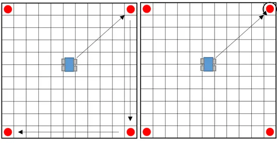
Figure 2.4: Exploration Figure 2.5: Exploitation

2.2.2 Exploitation vs exploration

For any mission were resources are scarce, there is a constant trade-off between exploration and exploitation. In probability theory this is often referred to as the K-armed bandit problem: Given a limited amount of resources, how should these resources be allocated between different choices to maximize the utility gain when the outcome is not fully known and can only be better understood by allocating the re-source to the different choices? [3] As an example, imagine a rover on the surface of Mars as illustrated in Fig 2.4 and 2.5. The dilemma fac-ing the operators back on Earth is the followfac-ing: Do you study known promising locations in hope of finding water as Fig 2.5 or do you cover as much ground as you can in hope of finding new promising loca-tions? This method is shown in Fig 2.4. While covering more ground can lead to an interesting find, it can also lead to the rover driving aimlessly around finding no interesting locations at all. A large sunk cost and something that could potentially jeopardize the success of the

(22)

mission. This trade-off becomes even more important for a spacecraft with a very limited amount of passes or a lander that only has one chance to increase the science return for the mission. The trajectories studied in this thesis have been picked to thoroughly study the entire spectrum in between these two extremes.

2.2.3 Spline trajectories

When referring to a spline in this thesis it means a piecewise polyno-mial parametric curve. Splines are advantageous since they produce a smooth trajectory that a robot can follow without demanding too much of the kinematics of the robot. Sharp turns necessitate large ac-celeration that might not be feasible for a given vehicle. This is even more important for a spacecraft with a large forward velocity that can-not be changed to maintain its orbital velocity. They are easy to con-struct and given a few selected points, or knots, a desired trajectory can be constructed.

Important desired properties of splines are localism, continuity, and correlation between shape and input parameters [23]. Continuity with regards to both the first and second derivative are desired to maintain a smooth trajectory and ensure that the vehicle can follow along the planned path. With localism, the desired property allows a change of one separate segment of the entire trajectory without changing the following segments. Lastly, the trajectory should follow the desired knot points closely. This enables the use of the trajectory by specifying important points that will be visited by the vehicle.

Choosing the type of spline to be used introduces a trade-off be-tween different properties. Example of popular splines are Hermite, Cubic Bezier, Catmull-Rom, and B-Splines [23]. All these are exam-ples of third degree polynomial splines. B-splines for example ensure C2 continuity along the entire trajectory but will not go through the points selected by the user. Cubic Bezier splines on the other hand will go through these knots but are not C2 continuous. The reason for this compromise is that both of these are constructed using 3rd de-gree polynomials. To include more properties, we need to increase the degree of freedom which requires the order of the polynomial used to be increased. This is not completely without any drawbacks how-ever. When using higher-order splines a phenomenon occurs where the curve starts to oscillate at the beginning and end points of the

(23)

tra-CHAPTER 2. BACKGROUND 13

jectory. This undesired effect is referred to as Runge’s phenomenon and is common for higher-order splines.

2.2.4 Adaptive trajectories

Adaptive trajectories have been studied in detail ranging from wheeled robots, airplanes, UAVs and even spacecraft. For airplanes and UAVs this has dealt with hazard avoidance, avoiding certain areas perceived as dangerous, encountering strong crosswinds or performing unex-pected emergency landings [27, 2]. For spacecraft this has been limited to trajectory optimization during atmospheric entry. This is a highly constrained phase of any mission and has dealt mostly with the pose of the spacecraft and the velocity-drag plane. The survey in this thesis is believed to be the first of its kind, studying how adaptive trajectories can be used to optimize the orbital trajectory of a spacecraft.

(24)

Chapter 3 Method

In this section the mission parameters for what would be a concept mission using the methods in this thesis are described. Secondly, the plume model that the spacecraft will traverse is presented together with the different trajectories that have been analyzed. In the end there is an outline of the testing procedure that have been used to evaluate these trajectories and compare them with each other.

3.1 Orbital parameters

The proximity of Enceladus to Saturn prevents the spacecraft from en-tering the unstable polar orbit around the moon [24]. An orbit that is traditionally used for reconnaissance missions and would let the spacecraft fly over the poles, letting the moon spin underneath it and cover most of the area over the poles. This means that the spacecraft would have to, just like Cassini, orbit around Saturn in a highly eccen-tric orbit. This also means that the spacecraft is likely to only have a few limited passes though the water plume.

The reason for using the adaptive trajectories proposed in this the-sis is to make the most out of these limited opportunities to investigate the plume. There is also a desire to probe the plume at an even lower altitude where the discretication of the jet sources are more apparent. While Cassini only flew by at an altitude of 50 km, the idea is to de-sign a mission going as low as 5 km. The altitudes that are investigated start at 25 km and then the altitude is lowered in increments to 20, 15, 10, and 5 km. A baseline altitude of 50 km is also included. This is the lowest altitude at which Cassini flew through the plume.

(25)

CHAPTER 3. METHOD 15

3.2 Plume model

3.2.1 Model selection

Since the first flyby of Enceladus, there have been a number of models that describe the nature of the plumes on Enceladus, regarding both location and activity [20]. Modelling these plumes is a significant un-dertaking that is worthy of a thesis in itself so for this thesis, where the interest is mostly in creating a realistic environment for the space-craft, an existing model will be used. While conducting this investiga-tion, a model is needed that can accurately represent a multiple-source plume. In addition, the model has to be able to incorporate the tidal stresses causing a varying activity in the density field. Therefore it is desirable to be able to control the number of active sources being used. An analytic model was chosen that have been compared with data from flybys that satisfies these requirements. More detail on this model is presented in the next section. There are other plume mod-els that have been produced that use more advanced fluid simulations that more accurately represent the density field. Examples are Direct Simulation Monte Carlo methods that have been used to model the plumes on both Enceladus and Europa [28, 11]. While these models provide a more accurate description, they are more complex and not as flexible. Given this and the requirement to have a model that can easily turn on and off sources, the added complexity outweigh the in-creased accuracy.

3.2.2 Analytical model used in this work

The plume model used in this thesis is based on the multiple-source model described in Dong et al. [4]. The model was created by fitting the results to data from Enceladus flybys E3, E5, and E7. This is a lin-ear superposition of individual sources that assume a radially flowing Maxwellian velocity distribution at the source:

fs(v) = ns ⇡3/2_v3 th exp{ [v2 x+ v2y+ (vz2 v02)]/vth2 } (3.1)

where nsis the number density at the source, v0 is the flow speed, and

vth=

q

2kT /mis the thermal speed. The model neglects both collisions

(26)

16 CHAPTER 3. METHOD

contribute to an error of roughly 10% for the flow velocity and source rate compared to taking this into account. They deem this an accept-able error that still yields an accurate density field for their model.

For the multiple-source model, the density away from the source can be described by the equation:

n =

98

X

n=1

ni(ri) (3.2)

where the density of each plume source, ni, can be modeled by:

ni(r, ✓) = nsrs2 ⇡r2 ⇢_{2M cos ✓} p ⇡ e M2 + + e M2

sin2✓[1 + 2M2_cos2_{✓][1 + erf (M cos ✓)]}

(3.3)

where M = v0/vth is the thermal Mach number. A source parameter

S is defined as S = nsrs2 cm 1 where ns is the particle density at the

source and rsis the diameter of the source. These parameters are

cho-sen after one of the Cassini flybys as S = 1.2 · 1022_cm 1_{with M = 1.8.}

Other studies that have compared this particular model to Cassini data have grouped sources by four different Mach numbers to give a better representation of the plume field [25]. For the study conducted in this paper, all sources are assumed to be identical. This is because there is currently no detailed documentation of the individual strength for each of the sources.

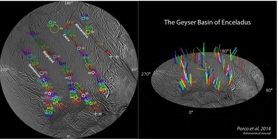
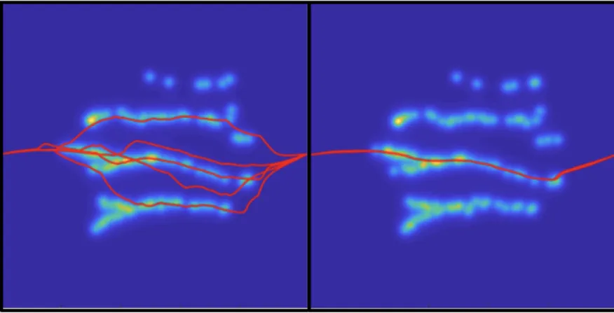
The locations of the plume sources are taken from Porco, DiNino, and Nimmo [17]. This is shown on the tiger stripes in Fig 3.1. In their modelling of each individual jet [17] they had the sources angled as can be seen in Fig 3.2. For the sake of simplicity, in this analysis the jet sources are assumed to always be perpendicular to the surface.

As discussed in the background section, a significant challenge for planning a mission to Enceladus is the uncertainty of the exact loca-tion and nature of these plume sources for any spacecraft wanting to make in-situ measurements by flying directly through them. To ac-curately represent the uncertainty of the jet sources in this study, two maps are used for each flyby. The density field is generated by as-suming that each plume source is located according to a distribution

(27)

Figure 3.1: Plume source locations Figure 3.2: Angle of each plume N(µ, ). This means that every time a map of the terrain is generated, each source have moved slightly to where it is expected to be found, µ. The spacecraft approaching the south polar terrain has one map of how it believes the plume field to look like a priori. Another map is then generated from the same distribution N(µ, ) and represents how the plume field actually looks like. The difference between these two maps is small but not negligible for a spacecraft flying through them. The spacecraft can choose to compare its a priori map to what it is measuring and after each flyby the spacecraft’s own map will be updated with the data it sampled of the actual density field. It com-bines the value in each pixel using 60% from the old map and 40% from what it sampled. These values were picked after running a few trials. The reason for this conservative approach, keeping more from the old map than is updated, is to avoid letting any noise picked up dictate the spacecrafts future planning. This could significantly disturb the spacecraft’s belief of the terrain.

The map of how the spacecraft believes the plume field to look like is updated from every state along the trajectory. The spacecraft will be equipped with a sensor with which it can measure the density in a close proximity in front of it. This sensing cone extends in front of the spacecraft and has an angle of 80 and all the density measurements within it is used to updated the a priori map.

The density field of the plume over the south pole is shown in Fig 3.3 and 3.4 that show the logarithm of the density at 10 and 50

(28)

km altitude, respectively. This also show the difference in the plume density field at lower altitudes, which is what is investigated in this thesis.

Figure 3.3: Plume field at 10 km Figure 3.4: Plume field at 50 km

3.3 Trajectories

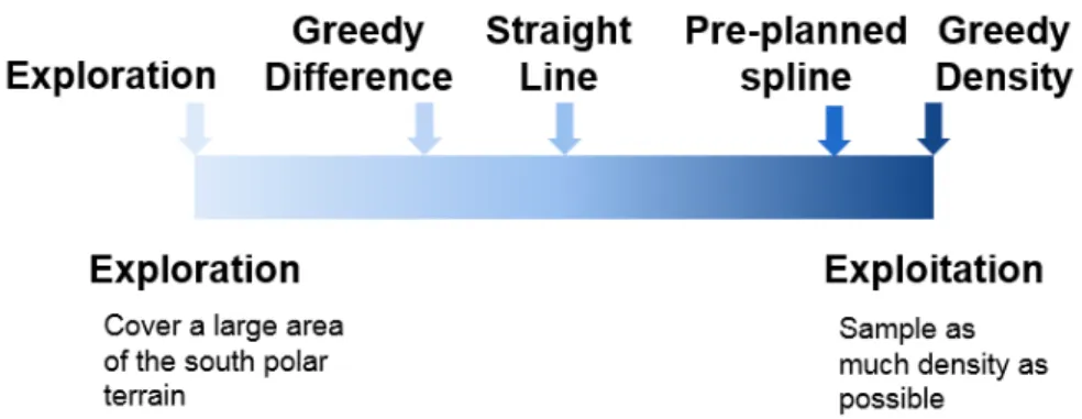
To investigate different means of traversing the south polar terrain of Enceladus, the spacecraft follows along a trajectory. The main goal of this study is to look at different ways of designing this trajectory and to do it in a way that span the spectrum between exploration and ex-ploitation as discussed in Section 2.2.2. The trajectories are placed on this spectrum in Fig 3.8. In total, five different trajectories have been designed and are compared with each other and evaluated. One of these is a straight line, detailed in 3.3.1, which consist of a traditional flyby where no steering is required. This is state-of-the-art for NASA and to date no other method has been attempted. The four other algo-rithms are what will be referred to as adaptive trajectories. These are divided into two categories: trajectories based on splines and greedy algorithms. These are described in sections 3.3.2. and 3.3.3, respec-tively. These in turn consist of two algorithms each: the two splines are based on sampling a large amount of density and explore a wide area. The two greedy algorithms are greedy on sampled density and difference between the two maps.

(29)

Figure 3.5: Straight-line trajectory

3.3.1 Straight line

A trajectory consisting of a straight line is studied as a benchmark to compare the adaptive trajectories to the traditional way of performing flybys. This is visualized in Fig 3.5. This is what Cassini and all other NASA missions would use. This trajectory flies over the south pole of Enceladus without any maneuvers or steering at all.

Figure 3.6: Left: Exploration, Right: A priori spline

3.3.2 Trajectories generated using splines

Every polynomial spline is generated as described in section 2.11. This is illustrated in Fig 3.6. The splines used are based on third degree polynomials to avoid Runge’s phenomenon as described in section 2.3.4. A total of 10,000 splines are generated for this step and the one

(30)

with the highest line integral density is chosen. After the spline with the highest utility has been selected, a random walk is performed on each knot point in order to try to increase the utility even further. The idea behind this is that if a trajectory has found a certain area to yield a high utility, by changing it slightly within that area a trajectory with an even higher science return could be found nearby.

A priori spline

The utility for this spline is to gather as much density along its path as possible. It does this by calculating the density based on the a priori map. The density it samples along the actual density field could vary from this, both positively and negatively. After each pass the a priori map is updated with what the spacecraft sensed during its previous pass at each altitude.

Exploration

The trajectory emphasizing exploration generates polynomial splines similar to that of the pre-planned splines in the previous paragraph. Instead of evaluating each spline by maximizing the sampled density, however, it rewards trajectories covering areas not yet visited at that altitude. This selection is not entirely random but prioritizes trajecto-ries that visit new areas while keeping delta-v requirements low. The main idea of this algorithm is that when performing several passes at each altitude the trajectories should cover a large area of the south pole.

3.3.3 Greedy trajectories

Greedy trajectories, while naive in their approach by design, can yield good result under the correct circumstances. The naive characteristic of greedy algorithms is that they chose the option that maximizes util-ity locally in each state, which might not always agree with the global maximum. When designing the greedy algorithms for this approach, a utility function is used:

utility = ↵_{· f(density) + · g(kinematic)} _{· ky}curr yplannedk (3.4)

The goal is to maximize the utility so the spacecraft takes the path that gathers the maximum density measure, which we have two of

(31)

Figure 3.7: Greedy algorithms. Left: Greedy on differences, Right: Greedy on density

in this study, and minimizes the deviation from its original trajectory yplanned. g(kinematic) is a constraint on the possible movements of the

spacecraft. Ideally these are taken by the actual dynamics of the vehi-cle, but since this is an early study, the sensing cone described in sec-tion 3.2.2. has been used to constrain the movement of the spacecraft. This is enough to ensure the spacecraft moves in a forward direction and avoid sharp turns. These trajectories are shown in Fig 3.7

Greedy on density

What separates the two greedy algorithms used in this study is the measure of utility, or the density measure. The trajectory that is greedy on density will in each state travel in the direction in which it senses the largest density. When presented with the same map, this algorithm always pursues the same path unless the density field has changed.

Greedy on difference

Similar to the previous algorithm but instead of pursuing the maxi-mum density in each state, this method pursues differences between the a priori map and the actual plume field. Given enough passes this should combine covering many plume sources that yield a high sam-pled density with covering a larger area to pursue differences between the two maps. When calculating the differences between the two maps, the absolute value of the difference is used. The reason for this is that a large negative difference should be rewarded as highly as a positive

(32)

one. Consider for example a location where the spacecraft would ex-pect a plume source but found none, this negative difference is also of value to learn more about the jets on Enceladus.

Figure 3.8: How the studied trajectories relate to each other on the exploration-exploitation spectrum.

3.4 Implementation/Test scheme

3.4.1 Delta-v calculations

The v calculations have been performed at every incremental change of the trajectory. Iterating through the trajectory the angle is calculated against the previous position. For the sake of simplicity, the spacecraft in this study will be assumed to follow a circular orbit around saturn. For a circular orbit, the v for an inclination change is calculated as:

v = 2v sin⇣ i

2 ⌘

(3.5) this is summed up for each step of the trajectory as the cumulative v for each trajectory.

3.4.2 Number of passes and altitudes investigated

The goal of this study is to quantify the result to be able to evaluate and compare these trajectories with each other. In order to do that a test scheme was designed that looks as follows:

1. 5 passes at each altitude are performed. Intuitively, algorithms that favour exploration will need several passes to do so while

(33)

greedy algorithms that favours the trajectory along the largest collected density will chose the same path each pass.

2. The interest of this survey is to study low altitudes so the study starts at 50 km which is the lowest altitude Cassini passed through and then incrementally lower the altitude stepwise. The evalua-tion will be at 50, 25, 20, 15, 10, 5 km.

3. In order to get useful statistics to evaluate the result, this was run 50 times for each set of passes at every altitude.

The metrics that was analyzed are:

• Total sampled density along the trajectory

• vto perform the desired trajectory

• How much area of the south polar terrain is covered • Sum of Squared Error for the believed map

3.4.3 Representation in simulation

Using the plume model from Dong et al. [4] we were able to generate a slice of the plume field for each altitude based on the locations from Porco, DiNino, and Nimmo [17]. The representation in the simulation will be a discrete representation by a 256⇥256 matrix where each pixel represents 1 km. This is a sufficient spatial resolution for this survey given the sampling capability of previous spectrometers and the speed of the spacecraft which is a few kilometers per second. This area cov-ers the entire south pole of Enceladus by starting just inside the 40 latitude that is considered to contain the south polar terrain. The spacecraft begins its trajectory just inside this area and ends it close to 40 latitude on the other side of the south pole. This is to leave some flexibility to the original trajectory design, as long as the spacecraft is aligned with those two points the adaptive trajectory segment is con-tained only to the south pole and does not need to be considered by the overall mission design.

(34)

Chapter 4 Results

This chapter presents the results from traversing the trajectories de-scribed in section 3.3. using the test framework and metrics outlined in section 3.4.

4.1 Sampled density at altitude

Figure 4.1 shows the average density across all 5 passes at each alti-tude. This has been collected for each pixel along the trajectory. There is a clear trend of increasing density toward the lower altitudes. The adaptive trajectories designed to sample more density outperform the traditional approach and the exploration focused trajectory.

4.2 Delta-v at altitude

Figure 4.2 shows the average delta-v across all 5 passes at each alti-tude. All trajectories show a significant cost in delta-v compared to a typical interplanetary mission that would use the straight line tra-jectory which has a cost of zero. The greedy trajectories have a large delta-v that would be expected given their naive approach. Both spline generated trajectories despite showing a large cost are both fairly con-sistent and given the large density sampled in the previous section, could be a promising alternative.

(35)

CHAPTER 4. RESULTS 25 5 10 15 20 25 30 35 40 45 50 Altitude (km) 0 0.5 1 1.5 2 2.5 3 Density (m -3)

×1028 Plume Density Sampled

Exploration Straight line Greedy Density Greedy Differences Spline

Figure 4.1: Density at each altitude

5 10 15 20 25 30 35 40 45 50 Altitude (km) 0 20 40 60 80 100 120 140 160 180 Delta-v (kms -1 Delta-v Required Exploration Straight line Greedy Density Greedy Differences Spline

Figure 4.2: Delta-v at each altitude

4.3 Density sampled per delta-v

The density sampled and delta-v are by themselves interesting, but it is much more valuable to look at trajectories that maximize density while keeping fuel costs low. Figure 4.3 shows the sampled density divided by delta-v and here the spline based method perform better.

(36)

26 CHAPTER 4. RESULTS 5 10 15 20 25 30 35 40 45 50 Altitude (km) 0 1 2 3 4 5 6 7 8 9 Density/ ∆ v (m -3/ms -1

×1023 Density normalized by delta-v

Figure 4.3: Density divided by delta-v

4.4 Coverage at altitude

Figure 4.4 shows the percentage of the map covered after all 5 passes at each altitude. As expected, the algorithm favoring exploration covers a large portion of the south polar terrain. The only other trajectory that manages to explore a larger portion of the map is the greedy algorithm using differences as a heuristic.

4.5 Sum of squared error at altitude

Figure 4.5 shows the sum of squared error between the map of what the spacecraft believes the terrain to look like vs the actual map. This is after the 5th pass at each altitude. It is expected for this to increase at lower altitudes as we know the discrete jet sources become more apparent. At larger altitudes the giant plume cloud is not as easy to distinguish between two different maps. The algorithms that cover the larger portion of the map also has a lower map error after the final pass.

(37)

CHAPTER 4. RESULTS 27 5 10 15 20 25 30 35 40 45 50 Altitude (km) 5 10 15 20 25 30 35 40 45 Percent Covered

Percentage of the south polar terrain covered

Figure 4.4: Map coverage at each altitude

5 10 15 20 25 30 35 40 45 50 Altitude (km) 50.5 51 51.5 52 52.5 53 53.5 54 54.5 55 55.5 log10 SSE (m -6 )

Sum of Squared Error

(38)

Chapter 5 Discussion

5.1 Discussion

Overall, keeping in mind the trade-off between exploration and ex-ploitation, the trajectories perform well in the areas they were designed to. Exploration covers the largest portion of the terrain and the greedy algorithms sample the most density.

One striking result is that the greedy algorithms perform so well in sampling density. Usually greedy algorithms pursue some local imum that does not guranatee that they will arrive at the global max-imum. In this study, greedy perform well using two different heuris-tics. The reason for this is likely the biased terrain the robot is travers-ing. The jet sources on the south pole are aligned in 4 tiger stripes where one of the stripes tend to have more sources. A spacecraft fol-lowing a greedy trajectory that will enter the south pole near this mid-dle stripe will follow it closely and thereby gather a significant amount of plume material. In hindsight, it would have been interesting to eval-uate these trajectories in a more unbiased, randomized terrain where a given amount of plumes had been spread out over an area similar in size to the south pole of Enceladus. The results of the algorithms there could then be compared to testing them in ’real-world terrains’ such as the south pole of Enceladus. The idea behind this is that an algo-rithm like greedy should not perform as well in a more randomized environment.

Worth discussing is also the significant delta-v costs of these trajec-tories. Out of plane changes are often avoided when designing space-craft tours because they necessitate large delta-v and for all of these

(39)

CHAPTER 5. DISCUSSION 29

trajectories there are many inclination changes that result in this high delta-v cost. Out of plane changes are a necessary step to being able to steer the spacecraft in orbit and will likely require significant steps of innovation within spacecraft propulsion before they are attempted in this fashion for an actual mission. It is also worth to consider that the way these trajectories were designed, large delta-v costs are not in any way penalized. The only one that had an heuristic which re-warded lower fuel consumption was the exploration algorithm. The other trajectories only rewarded a large sampled density, which they did achieve. There are two ways this can be implemented: firstly, the heuristic can reward trajectories with a lower delta-v cost. This would immediately lead to more low cost trajectories appearing among the high density ones. Secondly, the kinematic constraints on the greedy algorithms can be improved. Currently this is only limited to a steer-ing radius of 40 but more severe constraints can preferably be used to make the spacecraft not jitter around as much, leading to a smoother trajectory and lower delta-v requirements.

5.2 Future work

Part of the work done during this thesis was to try and find an algo-rithm that could outperform the traditional trajectory algoalgo-rithms sur-veyed already. One attempt to do this was to simulate the plume field after each pass in order to find one that closely matched what had been seen by the spacecraft during the previous pass. The idea is that the pre-planned spline trajectory would perform even better using a more accurate a priori map. Unfortunately all attempts at this yielded unsuc-cessful results. The overall science return did not improve: sampled density was not higher than when using the old a priori map and there was no noticeable difference in fuel consumption.

This work was done within a group simulating icy moons in Gazebo using ROS, Robotic Operating System, a robotics framework, with C++. This thesis was successful in developing a framework for per-forming these trajectories and the testing of them can be changed with ease to different scenarios. Hopefully future students can work on implementing these trajectories within Gazebo instead of using MAT-LAB.

(40)

30 CHAPTER 5. DISCUSSION

5.3 Conclusion

The adaptive trajectories perform well in each respective area of what they were designed to do: increase the science return with a limited amount of flybys of Enceladus. This science return depend on the mis-sion profile and can be either mapping the south pole of the moon or flying through the plumes, sampling a large amount of plume mate-rial. One concern for missions implementing this methodology is the fuel costs and lack of experience using autonomous capabilities in sit-uations like the one presented in this study. Only time can tell but with innovation in the areas of spacecraft propulsion and autonomy, hope-fully autonomy will become a natural part of any mission to space.

(41)

Bibliography

[1] P. D. Alex and S.A. Kattenhorn. “A fracture history on Enceladus provides evidence for a global ocean”. In: Geophysical Research

Letters 38.18 (2011).DOI: 10.1029/2011GL048387.

[2] I. Alonso-Portillo and E. M. Atkins. “Adaptive Trajectory Plan-ning for Flight Management Systems”. In: AAAI Technical Report (2001).

[3] D. A. Berry and B. Fristedt. Bandit Problems: Sequential Allocation

of Experiments. Springer Science & Business Media, 2013. ISBN:

978-94-015-3711-7.

[4] Y. Dong et al. “The water vapor plumes of Enceladus”. In: Journal of Geophysical Research 116 (2011), A10204.

[5] K. P. Hand et al. Europa Lander Lander Study 2016 Report. 2016. [6] Candice J. Hansen et al. “Enceladus’ Water Vapor Plume”. In:

Science 311.5766 (2006), pp. 1422–1425.ISSN: 0036-8075.DOI: 10.

1126/science.1121254.

[7] M.M. Hedman et al. “An observed correlation between plume activity and tidal stresses on Enceladus”. In: Nature 500 (2013), pp. 182–184.

[8] H-W. Hsu et al. “Ongoing hydrothermal activities within Ence-ladus”. In: Nature 519 (2015), pp. 207–210.

[9] NASA Jet Propulsion Laboratory. Enceladus: Ocean Moon. 2017.

URL: https://saturn.jpl.nasa.gov/science/enceladus/

(visited on 05/27/2018).

[10] S. M. LaValle. Planning Algorithms. Cambridge, U.K.: Cambridge

University Press, 2006.ISBN: 978-05-218-6205-9.

(42)

32 BIBLIOGRAPHY

[11] Zheng Li, Rohit Dhariwal, and D. A. Levin. “DSMC simulation of near-field enceladus plumes from tiger stripe fractures”. En-glish (US). In: 44th AIAA Thermophysics Conference. 2013.

[12] ENCELADUS LIFE FINDER: THE SEARCH FOR LIFE IN A HAB-ITABLE MOON. 46th Lunar and Planetary Science Conference. Texas, United States, Mar. 2015.

[13] NASA. What’s Next For NASA? 2018. URL: https : / / www .

nasa.gov/about/whats_next.html(visited on 09/16/2018).

[14] K. D. Pang et al. “The E ring of Saturn and satellite Enceladus”. In: Journal of Geophysical Research: Solid Earth 89.B11 (1984), pp. 9459– 9470.

[15] C. C. Porco et al. “Cassini Observes the Active South Pole of

Enceladus”. In: Science 311.5766 (2006), pp. 1393–1401.ISSN:

0036-8075. DOI: 10.1126/science.1123013.

[16] Enceladus 101Geysers : P hantoms?Hardly. American Geophys-ical Union, Fall Meeting 2015. San Francisco, United States, Dec. 2015.

[17] C. Porco, D. DiNino, and F. Nimmo. “How the Geysers, Tidal Stresses, and Thermal Emission Across the South Polar Terrain of Enceladus are Related”. In: The Astronomical Journal 148 (2014), 3.

[18] Carolyn C. Porco, Luke Dones, and Colin Mitchell. “Could It Be Snowing Microbes on Enceladus? Assessing Conditions in Its Plume and Implications for Future Missions”. In:

Astrobiol-ogy 17.9 (2017). PMID: 28799795, pp. 876–901. DOI: 10.1089/

ast.2017.1665.

[19] L Roth et al. “Transient Water Vapor at Europa’s South Pole”. In:

Science 343.6167 (2014), pp. 171–174. ISSN: 0036-8075. DOI: 10.

1126/science.1247051.

[20] J. Saur et al. “Evidence for temporal variability of Enceladus’ gas jets: Modelling of Cassini Observations”. In: Geophysical Research Letters 35 (2008).

[21] J. N. Spitale and C. C. Porco. “Association of the jets of Ence-ladus with the warmest regions on its south-polar fractures”. In: Nature 449 (2007), pp. 695–697.

(43)

BIBLIOGRAPHY 33

[22] J.N. Spitale et al. “Curtain eruptions from Enceladus’ south-polar terrain”. In: Nature 521 (2015), pp. 57–60.

[23] C. Sprunk. “Planning Motion Trajectories for Mobile Robots Us-ing Splines”. MA thesis. Germany: Albert-Ludwigs-Universität Freiburg, 2008.

[24] Study on the Stability of Science Orbits of Enceladus. 38th Annual Meeting of the Division for Planetary Sciences. Pasadena, United States, Oct. 2006.

[25] B. D. Teolis et al. “Enceladus Plume Structure and Time Variabil-ity: Comparison of Cassini Observations.” In: Astrobiology 17(9) (2017), pp. 926–940.

[26] J. Hunter Waite et al. “Cassini finds molecular hydrogen in the Enceladus plume: Evidence for hydrothermal processes”. In:

Sci-ence 356.6334 (2017), pp. 155–159.ISSN: 0036-8075.

[27] Adaptive Trajectory Tracking Control of a Wheeled Mobile Robot via Lyapunov Techniques. The 30th Annual Conference of the IEEE Industrial Electronics Society. Busan, Korea, Nov. 2004.

[28] S. K. Yeoh et al. “A Hybrid Simulation of the Gas/Particle Plume of Enceladus”. In: Journal of Geophysical Research 116 (2011), A10204.

(44)

Appendix A

Scatter plots of all trajectories

These scatter plots can be used to study the relationship between all the different metrics and compare them to each other for every alti-tude. 0 1 2 3 4 Density (m-3₎ _×1028 0 10 20 30 Density (m -3) 0 1 2 3 4 ×1028 0 50 100 150 Delta-v (m/s) 0 1 2 3 4 ×1028 0 0.2 0.4 0.6 Coverage (%) 0 1 2 3 4 ×1028 54.5 55 55.5 SSE (m -6) 0 50 100 150 Fuel (m/s) 0 1 2 3 4×1028 0 50 100 150 0 20 40 60 0 50 100 150 0 0.2 0.4 0.6

Exploration Straight Line Greedy Density Greedy Difference Spline

0 50 100 150 54.5 55 55.5 0 0.2 0.4 0.6 Coverage (%) 0 1 2 3 4×1028 0 0.2 0.4 0.6 0 50 100 150 0 0.1 0.2 0.3 0.4 0 20 40 60 0 0.2 0.4 0.6 54.5 55 55.5 54.5 55 55.5 SSE (m-6₎ 0 1 2 3 4×1028 54.5 55 55.5 0 50 100 150 54.5 55 55.5 0 0.2 0.4 0.6 54.5 55 55.5 0 5 10

Figure A.1: Scatter plot of all trajectories at 5 km altitude

(45)

APPENDIX A. SCATTER PLOTS OF ALL TRAJECTORIES 35 0 0.5 1 1.5 2 Density (m-3₎ ×1028 0 10 20 30 Density (m -3) 0 0.5 1 1.5 2 ×1028 0 50 100 150 Delta-v (m/s) 0 0.5 1 1.5 2 ×1028 0 0.2 0.4 0.6 Coverage (%) 0 0.5 1 1.5 2 ×1028 53 53.5 54 54.5 SSE (m -6) 0 50 100 150 Fuel (m/s) 0 0.5 1 1.5 2×1028 0 50 100 150 0 20 40 60 0 50 100 150 0 0.2 0.4 0.6

0 50 100 150 53 53.5 54 54.5 0 0.2 0.4 0.6 Coverage (%) 0 0.5 1 1.5 2×1028 0 0.2 0.4 0.6 0 50 100 150 0 0.2 0.4 0.6 0 20 40 60 0 0.2 0.4 0.6 53 53.5 54 54.5 53 53.5 54 54.5 SSE (m-6₎ 0 0.5 1 1.5 2×1028 53 53.5 54 54.5 0 50 100 150 53 53.5 54 54.5 0 0.2 0.4 0.6 53.5 54 54.5 0 5 10 15

(46)

36 APPENDIX A. SCATTER PLOTS OF ALL TRAJECTORIES 0 5 10 15 Density (m-3_{) ×10}27 0 10 20 30 Density (m -3) 0 5 10 15 ×1027 0 50 100 150 200 Delta-v (m/s) 0 5 10 15 ×1027 0 0.2 0.4 0.6 Coverage (%) 0 5 10 15 ×1027 52.5 53 53.5 SSE (m -6) 0 50 100 150 200 Fuel (m/s) 0 5 10 15×1027 0 50 100 150 200 0 20 40 60 0 50 100 150 200 0 0.2 0.4 0.6

0 50 100 150 200 52.5 53 53.5 0 0.2 0.4 0.6 Coverage (%) 0 5 10 15×1027 0 0.2 0.4 0.6 0 50 100 150 200 0 0.2 0.4 0.6 0 20 40 60 0 0.2 0.4 0.6 52.5 53 53.5 52.5 53 53.5 SSE (m-6₎ 0 5 10 15×1027 52.5 53 53.5 0 50 100 150 200 52.5 53 53.5 0 0.2 0.4 0.6 52.5 53 53.5 0 5 10

(47)

APPENDIX A. SCATTER PLOTS OF ALL TRAJECTORIES 37 0 5 10 Density (m-3_{) ×10}27 0 10 20 30 Density (m -3) 2 4 6 8 10 ×1027 0 50 100 150 200 Delta-v (m/s) 2 4 6 8 10 ×1027 0 0.2 0.4 0.6 Coverage (%) 2 4 6 8 10 ×1027 52 52.5 53 53.5 SSE (m -6) 0 50 100 150 200 Fuel (m/s) 2 4 6 8 10×1027 0 50 100 150 200 0 20 40 60 0 50 100 150 200 0 0.2 0.4 0.6

0 50 100 150 200 52 52.5 53 53.5 0 0.2 0.4 0.6 Coverage (%) 2 4 6 8 10×1027 0 0.2 0.4 0.6 0 50 100 150 200 0 0.2 0.4 0.6 0 20 40 60 0 0.2 0.4 0.6 52 52.5 53 53.5 52 52.5 53 53.5 SSE (m-6₎ 2 4 6 8 10×1027 52 52.5 53 53.5 0 50 100 150 200 52 52.5 53 53.5 0 0.2 0.4 0.6 52 52.5 53 53.5 0 5 10

(48)

38 APPENDIX A. SCATTER PLOTS OF ALL TRAJECTORIES 2 4 6 8 Density (m-3_{) ×10}27 0 10 20 30 40 Density (m -3) 2 4 6 8 ×1027 0 50 100 150 200 Delta-v (m/s) 2 4 6 8 ×1027 0 0.2 0.4 0.6 Coverage (%) 2 4 6 8 ×1027 51.5 52 52.5 53 SSE (m -6) 0 50 100 150 200 Fuel (m/s) 2 4 6 8×1027 0 50 100 150 200 0 20 40 60 0 50 100 150 200 0 0.2 0.4 0.6

0 50 100 150 200 51.5 52 52.5 53 0 0.2 0.4 0.6 Coverage (%) 2 4 6 8×1027 0 0.2 0.4 0.6 0 50 100 150 200 0 0.2 0.4 0.6 0 20 40 60 0 0.2 0.4 0.6 51.5 52 52.5 53 51.5 52 52.5 53 SSE (m-6₎ 2 4 6 8×1027 51.5 52 52.5 53 0 50 100 150 200 51.5 52 52.5 53 0 0.2 0.4 0.6 51.5 52 52.5 53 0 5 10

(49)

APPENDIX A. SCATTER PLOTS OF ALL TRAJECTORIES 39 2 3 4 5 6 Density (m-3_{) ×10}27 0 10 20 30 40 Density (m -3) 2 3 4 5 6 ×1027 0 50 100 150 200 Delta-v (m/s) 2 3 4 5 6 ×1027 0 0.2 0.4 0.6 Coverage (%) 2 3 4 5 6 ×1027 50 50.5 51 51.5 52 SSE (m -6) 0 50 100 150 200 Fuel (m/s) 2 3 4 5 6×1027 0 50 100 150 200 0 20 40 60 0 50 100 150 200 0 0.2 0.4 0.6

0 50 100 150 200 50 50.5 51 51.5 52 0 0.2 0.4 0.6 Coverage (%) 2 3 4 5 6×1027 0 0.2 0.4 0.6 0 50 100 150 200 0 0.2 0.4 0.6 0 20 40 60 0 0.2 0.4 0.6 50 50.5 51 51.5 52 50 50.5 51 51.5 52 SSE (m-6₎ 2 3 4 5 6×1027 50 50.5 51 51.5 52 0 50 100 150 200 50 50.5 51 51.5 52 0 0.2 0.4 0.6 50 50.5 51 51.5 52 0 5 10

(50)

(51)

(52)

TRITA TRITA-EECS-EX-2018:312

Investigating Adaptive Trajectories to Explore Water Plumes on Icy Moons

Investigating Adaptive Trajectories

to Explore Water Plumes on Icy

Moons

MARCUS ACKLAND

Investigating Adaptive

Trajectories to Explore Water

Plumes on Icy Moons

MARCUS ACKLAND

Abstract

Sammanfattning

Acknowledgement

Contents

Chapter 1

Introduction

1.1 Motivation

1.2 Problem statement

1.3 Contribution

1.4 Limitations

1.5 Outline

Chapter 2

Background

2.1 Enceladus

2.1.1 Cryovolcanic activity

2.1.2 Indications of life

2.1.3 Cassini flybys

2.1.4 Plans for future missions to icy moons

2.2 Trajectory Planning

2.2.1 Open vs closed feedback

2.2.2 Exploitation vs exploration

2.2.3 Spline trajectories

2.2.4 Adaptive trajectories

Chapter 3

Method

3.1 Orbital parameters

3.2 Plume model

3.2.1 Model selection

3.2.2 Analytical model used in this work

3.3 Trajectories

3.3.1 Straight line

3.3.2 Trajectories generated using splines

3.3.3 Greedy trajectories

3.4 Implementation/Test scheme

3.4.1 Delta-v calculations

3.4.2 Number of passes and altitudes investigated

3.4.3 Representation in simulation

Chapter 4

Results

4.1 Sampled density at altitude

4.2 Delta-v at altitude

4.3 Density sampled per delta-v

4.4 Coverage at altitude

4.5 Sum of squared error at altitude

Chapter 5

Discussion

5.1 Discussion

5.2 Future work

5.3 Conclusion

Bibliography

Appendix A

Scatter plots of all trajectories