Traction Adaptive trajectory planning for autonomous racing

(1)

Traction Adaptive trajectory

planning for autonomous

racing

FELICIA ABOUD VIEIDER

ANIRUDH NARASIMHA KULKARNI

KTH ROYAL INSTITUTE OF TECHNOLOGY

(2)

Traction Adaptive trajectory planning for

autonomous racing

Felicia Aboud Vieider

Anirudh Narasimha Kulkarni

Master of Science Thesis TRITA-ITM-EX 2020:444 KTH Industrial Engineering and Management

Machine Design SE-100 44 STOCKHOLM

(3)

(4)

Examensarbete TRITA-ITM-EX 2020:444

Greppadaptiv rörelseplanering för autonom racing

Felicia Aboud Vieider Anirudh Narasimha Kulkarni

Godkänt Examinator DeJiu Chen Handledare Lars Svensson Uppdragsgivare AFRY AB Kontaktperson Anders Mattsson

Sammanfattning

De senaste åren har den autonoma fordons industrin genomgått en stor utveckling genom forskning, företag har gjort stora investeringar för att förbättra teknologin för att kunna nå den privata marknaden. Industrin och akademin jobbar fortfarande för att göra autonoma bilar säkra, pålitliga och robusta. Autonom racing tillhandahåller en plattform för att förbättra tekniken så att den kan utnyttja fordonets fulla fysiska förmåga i ett brett spektrum av driftsförhållanden. Flera funktioner krävs för att göra bilen autonom, detta arbete fokuserar på rörelseplaneringsmodulen för autonom racing. Vi har utvärderat hur rörelseplanerings algoritmen presterar vid användning av en dynamisk modell med dynamiska begräsningar.

Utvärderingen är baserad på ett ramverk för optimal rörelseplanering [1] vilken löser optimerings problemet genom användning av "Sampling Augmented Real Time Iteration (SAARTI) motion planning scheme". Fyra olika modeller jämfördes vilka inkluderade en dynamisk cykelmodell med både statiska och dynamiska begränsningar. De parametrar som påverkade prestandan identifierades, och avvägningen mellan modell komplexitet och planerings horisont undersöktes genom att studera skillnader i prestanda för olika parameter konfigurationer. Generaliserbarhet av resultaten undersöktes genom att studera prestandan för olika parameter konfigurationer under olika körförhållanden.

Batch simuleringar utfördes för att ta hänsyn till många olika scenarion, för att säkerställa att resultaten var så nära verkligheten som möjligt. Simuleringarna visade att användning av dynamiska begränsningar vid rörelse planering förbättrar prestandan jämfört med att använda statiska begränsningar vid extrema körförhållanden.

Observation av resultaten från simuleringarna visade att användning av den grepp adaptiva modellen resulterade i robust och konsistent prestanda. Att kombinera estimering av friktion och samtidigt ta hänsyn till en varierande normal kraft, ökar förmågan att planera för variationer i friktion, minskar chansen att bilen kör av vägen och förbättrar varvtiden.

(5)

(6)

Master of Science Thesis TRITA-ITM-EX 2020:444

Traction Adaptive trajectory planning for autonomous racing

Felicia Aboud Vieider Anirudh Narasimha Kulkarni

Approved Examiner DeJiu Chen Supervisor Lars Svensson Commissioner AFRY AB Contact person Anders Mattson

Abstract

The autonomous driving industry has undergone leaps and bounds of research to reach the mainstream market, with major players investing heavily to improve the technology further. Industry and academia are currently working to make the technology safe, reliable and robust. Autonomous racing provides this opportunity, to improve the technology to the point, where it can utilize the full physical capability of the vehicle in a wide range of operational conditions. Multiple functionalities are required to make the car autonomous, this thesis focuses on the path planning module for autonomous racing. We evaluated the performance of dynamic models, using different adaptive dynamic constraints, implemented for path planning.

The evaluation is based on framework for optimization based motion planning[1] The optimization problem is solved by "Sampling Augmented Real Time Iteration (SAARTI) motion planning scheme". Four different models were studied during this thesis and include dynamic bicycle models, with static and dynamic constraints. Parameters affecting the planning performance were identified, and the trade-off between model complexity and planning horizon, was investigated by varying these parameters and the differences in performance was studied. The generalizability of results for different driving conditions was investigated for these parameter configurations.

Batch simulations were performed to account for various possible scenarios of different parameter configurations, to ensure results closest to reality. The simulation was conducted with, hardware in the loop setup running the planning node, to get a realistic estimation of the computation resources. Batch simulations were instrumental in showing interesting trends of how the input parameters affected the planning performance. Simulations provided extensive proof of the different dynamic constraints improving the planning performance, over the basic dynamic model under extreme driving conditions.

When reviewing the results from the simulations, the traction adaptive model showed robust and consistent performance. The results showed that combining friction estimation and load adaption, increased the ability to plan for local variations, reduced failure and improved laptime. When designing a planner for a race car that is exposed for local variations, the friction estimation is needed to reduce errors and the load adaption is needed for better handling of the vehicle to perform critical maneuvers.

(7)

(8)

iv

Acknowledgements

We would like to express our appreciation and gratitude to all the people who made this thesis possible by their contributions. Firstly, we thank our KTH supervisor Lars Svensson who contributed with both the planning framework and his time to provide feedback throughout our work. The discussions about theory and results were instrumental in completing the thesis. We would also like to thank our AFRY supervisor Stefan Ionescu and manager Anders Matt-son for welcoming us at the office and supporting our work by weekly updates to help our project go forward and by giving us feedback to make improve-ments on the work done. Finally, we would like to thank KTH, our course supervisor Fredrik Asplund for helping us developing the research question, our examiner DeJiu Chen, and our opponents Sara Soltaniah and Johanna Ol-las for their feedback to finalize and refine our work.

(9)

Contributions

This thesis was completed by the authors as part of their Masters of Science in Mechatronics at Kungliga Tekniska Högskolan (KTH). When preparing for the simulations the distribution of work is 50% for both members. All sections were worked through together. Work was done in collaboration using paired programming and discussion. Both members have an equal understanding of the system and theory governing it. The largest aspects of individual work was reading papers for the theoretical section or writing small functions. In addition, the simulations was done by Anirudh and data visualizations was done by Felicia.

(10)

List of Figures

1.1 Design flow of general Case Study [8] . . . 5

3.1 Illustration of the bicycle model showing the relation between Global X-Y frame and Frenet frame. s denotes the progress along the centerline of the lane . . . 13

3.2 An illustration of the velocity vector (represented by the red arrow) and the angle relative the rear wheel . . . 15

3.3 Lateral tire force as a function of slip angle for different road conditions. [30] . . . 16

3.4 Force distribution - side view [27] . . . 17

3.5 Sampling augmented adaptive RTI algorithm [1] . . . 20

4.1 The S- and U- curves with different radius which form the cases of the case study, the radius of the curves is denoted as r . . . 22

4.2 Failure for different N values using TA . . . 23

4.3 Effect on NA when varying µ-sd . . . 23

4.4 Hardware in the loop setup for batch simulations . . . 27

4.5 System architecture . . . 28

4.6 Visualisation of the planned path and the sample trajectories using RVIZ . . . 28

4.7 A visualization of an s-shaped track with varying friction sec-tions. The colorbar in the bottom shows the colormapping for the friction coefficient sections in the track . . . 30

5.1 A sample of succeeded laps for NA on an S shaped track with radii= 20 and µ-sd = 0.2. Color mapping on the vehicle path shows the longitudinal velocity in m/s and color mapping on the track shows the real tire-road friction coefficient µ, NA uses an values of µ = 1.6 for planning . . . 33

(13)

5.2 Plots showing failure and laptime vs planning horizon N. Lines illustrate mean value to combine the results for all input pa-rameters and the colored area around the lines illustrates the 68% confidence interval for on each value of N . . . 34 5.3 Laptime and failure visualized in the same graph to view the

change in both laptime and failure . . . 36 5.4 Planning time and failure. Planning time is defined as the

av-erage planning time for a lap, the lines defined the mean result for all combinations of input parameters, and the shaded area around the curves shows the standard deviations in the results . 36 5.5 Successful laps for different planning horizons using NA model 37 5.6 Boxplot showing the distribution of planning time for different

planning horizons denoted as N . . . 38 5.7 Successful laps for different planning horizons using LA . . . 39 5.8 Successful laps for different planning horizons using FA . . . 39 5.9 Successful laps for different planning horizons using TA . . . 39 5.10 Failure graph filtered by friction coefficient variance . . . 40 5.11 Laptime graph filtered by friction coefficient variance . . . 41 5.12 Planning time graph filtered by friction coefficient variance . . 41 5.13 Differences between different variances in friction . . . 42 5.14 Failed path visualised on varying friction track for NA model

on track with µ-sd = 0.6 . . . 43 5.15 Failed path visualised on varying friction track for TA . . . . 44 5.16 Failed path visualised on varying friction track for FA . . . . 44 5.17 Failed path visualised on varying friction track for LA . . . . 45 5.18 Failure graph filtered by track shape . . . 46 5.19 Failure graph filtered by track radius . . . 46 5.20 Laptime graph filtered by track radius . . . 47 5.21 Lap plot showing failed laps for NA model on U curve with

µ-sd = 0.6 . . . 47 5.22 Lap plot showing failed laps for NA model on S curve with

µ-sd = 0.6 . . . 48 5.23 Lap plot showing failed laps for TA model on U curve with

µ-sd = 0.6 . . . 49 5.24 Lap plot showing failed laps for TA model on S curve with

µ-sd = 0.6 . . . 49 5.25 Lap plot showing failed laps for LA model on S curve with

(14)

LIST OF FIGURES x

5.26 Lap plot showing failed laps for FA model on S curve with µ-sd = 0.6 . . . 50

(15)

3.1 Table showing the difference between the four models . . . 12 4.1 Table showing the input variables and their levels . . . 24 4.2 Table showing the experimental units . . . 24 5.1 Table presenting results at point of failure for each model, the

result is an average for all track shapes and radius . . . 35

(16)

Acronyms

DoF Degrees of freedom. 8

FSSIM Formula Student Simulator. 6, 7, 26, 27 MPC Model predictive control. 2, 9, 10

NMPC Nonlinear Model predictive control. 10, 11 ROS Robot Operating System. 7, 25–27

RTI Real Time Iteration Sequential Quadratic programming. 11, 18, 19 SAARTI Sampling Augmented Real Rime Iteration. 11

SLAM Simultaneous localization and mapping. 6

(17)

Introduction

1.1 Background

Autonomous driving has undergone a lot of research in recent years, to make it safe and reliable [2]. Some functionalities involved in autonomous driv-ing, include perception, localization, path planndriv-ing, and path following. The dream of large scale commercial deployment of autonomous cars is closer to reality today, with the industry taking a keen interest. AFRY as an engineer-ing, design, and advisory company, works together with other companies to improve and develop the technology. This thesis was conducted with AFRY Sweden and focuses on path planning for autonomous racing to improve the autonomous driving competence of the company.

In autonomous racing, cars drive in an environment void of human interven-tion and therefore provides a platform to develop and test new technologies, pushing the limits of vehicle capabilities. This setup ensures a low risk of human injuries [3]. Racing is a challenging task for an autonomous system. Primarily due to the need for handling the vehicle close to its stability limits to reach high speeds, in cases like sharp corners or slippery surfaces. Also, the dynamic limits of the vehicle are time-dependent due to local variations in terms of varying road conditions, and high accelerations causing varying distribution of normal force. Implementation of a real-time system with the need for fast computations on an embedded platform with limited computa-tional power makes the task even more challenging [4].

Trajectory planning is essential in autonomous vehicles, a trajectory describes how configurations, for example, position, and velocity of the vehicle will

(18)

CHAPTER 1. INTRODUCTION 2

evolve with time. By using the input from the surroundings it is possible to predict feasible trajectories for the vehicle. Feasible and optimal path plan-ning has been studied extensively, and a large number of algorithms have been developed [5]. This thesis will be based on the thesis done by Ionescu and Jon-sson [6], which used an algorithm based on Model predictive control (MPC) for trajectory planning. One of the factors affecting this planning method is, the selection of the vehicle model. Ionescu and Jonsson [6] showed improved performance for planning, in terms of laptime, when increasing the model complexity from a kinematic bicycle model to a dynamic bicycle model. This thesis [6] stresses the need for having a more complex way of describing the constraints on the tire forces to improve the constraints at high accelerations. Another factor affecting performance is the planning horizon[6], which de-cides how far ahead in time planning will be done. The previous thesis inves-tigated the trade-off between model accuracy and planning horizon, by em-ploying complex models. We extend this work by using a dynamic model with dynamic constraints adapting to time-varying traction limitations, and investigate if it improved the planning performance in real-time.

1.2 Problem description

Optimal performance in autonomous racing is achieved when the vehicle op-erates close to its physical limits [7]. To fully use the physical capabilities of the vehicle an accurate description of the dynamics and dynamic constraints are required [1]. The dynamic model used by Ionescu and Jonsson [6] is based on the assumption of static force constraints on the tires. This model will only be an accurate representation of the system when the vehicle is operating in static traction conditions of the road.

Increased model complexity for trajectory planning will permit the cars to reach their physical limits in terms of speed and control. However, given limited computational resources, a more complex vehicle model would also increase the computational time which would negatively affect performance in real-time applications. Planning horizon length decides for how many steps the planning will be done, a high planning horizon allows the planner to see further and allow for better planning. At the same time, longer planning hori-zon leads to more computations and a longer planning time. Ionescu and Jon-sson [6] show that the optimal planning horizon is varying with the shape of the track [6]. Planning horizon length and model accuracy, both affect the

(19)

computation time and performance of the trajectory planner, meaning there is a trade-off between model accuracy and planning horizon.

Most models used for trajectory planning is based on assuming a constant tire-road friction coefficient and normal forces acting on the tires. Although the dynamic limits are typically varying with time due to local variations in terms of road, tire condition, temperature and distribution of the normal force. Hence, Svensson et al. [1] proposed to incorporate, an adaptation of tire force constraints of the vehicle at run time for motion planning to avoid obstacles. The traction adaptive algorithm allowed the vehicle to avoid obstacles with in-creased capacity, in comparison to an equivalent non-adaptive control scheme [1]. Thus we hypothesize that including traction adaptation in trajectory plan-ning for racing will improve performance, in terms of increased laptime while keeping the vehicle inside the track, compared to using static constraints.

1.3 Hypothesis

Four types of constraints on the maximum tire force will be examined: • Static constraints

• Dynamic constraints depending on friction estimation • Dynamic constraints depending on the normal load

• Dynamic constraints depending on both friction estimation and varying normal load

Using dynamic constraints require more computations, meaning a limited com-putation force could result in a longer comcom-putation times.

We hypothesize that all models will have decreased failure with higher plan-ning horizons although there will be a trade-off when the planplan-ning time gets close the sample time, and failure will start to increase with higher planning horizons. The model using static constraints will have a lower increase in planning time and therefore be less negatively affected by increased planning horizon.

Using static constraints will allow for higher planning horizon at the point of failure compared to dynamic constraints, but will have high failure when there are high variations in surface friction. Models using friction estimation will

(20)

lead to lower failure due to the decreased environmental error. Models with dy-namic constraints considering varying normal load without friction estimation permit higher accelerations resulting in shorter laptime. Models running close to physical limits become prone to model errors, hence resulting in higher fail-ure when considering varying normal load. Using dynamic constraints with both friction estimation and adaption to normal load will give lower failure compared to only normal load adaption and a lower laptime compared to only using friction estimation.

1.4 Research Question

Previous research[6] has shown that increased accuracy and planning hori-zon improves planning performance while causing an increase in computation time, when given limited computational resources. Therefore, considering a real-time application. Increased computation time will at some point affect the vehicle’s performance negatively, as the benefit of high plan quality will be outweighed by extensive planning delay. Ionescu and Jonsson [6] showed that the optimal planning horizon is varying with the features of the racing track, and that, the S-curve, a U-turn, and a double U-turn had the most im-pact on planning horizon.

Optimal trade-off between model accuracy and planning horizon length should optimize laptime and failure. At the same time, utilizing all computational re-sources available should at times mean that the vehicle is operating just at the point of failure, i.e. that the latency and planning are both just enough to keep the vehicle from going off the track. Given these circumstances:

– What are the implications of using a dynamic model with dynamic con-straints (traction adaption) compared to a dynamic model with static constraints?

– Investigated for the above mentioned race track features, is it possible to generalize these implications for an arbitrary race track?

1.5 Methodology

Using case study is feasible when studying “a contemporary phenomenon within its real-life context, especially when the boundaries between the phe-nomenon and context are not clearly evident” [8]. To answer the research

(21)

ques-tion the performance of the path planner was to be evaluated during different scenarios and input parameters. Case study was a suitable choice of research method since this method allowed control of the real-life context to investi-gate how the shape of the track affects the result. Case studies permit in-depth study of specific cases [9], each case was evaluated by means of quantitative metrics like laptime and success rate of path planning.

Figure 1.1: Design flow of general Case Study [8]

Figure 1.1 shows the important steps that were required in making a case study. During the initial design phase, a hypothesis was set up from the existing liter-ature. The models and planning algorithm was set up during this phase. The next step involved the selection of different cases and setup of the simulation environment. The research investigated the implications of different vehicle models and if these implications were general for various tracks. Hence, dif-ferent track shapes were chosen as cases. Difdif-ferent sets of input variables and models were evaluated for these track sections by running simulations. Inputs included planning horizon and friction estimate accuracy, and the output was quantified as laptime and fail rate. The different parameters were plotted to observe interesting behavior and relations, which provided quantitative data for basing qualitative analysis. The qualitative analysis answered the initial hypothesis and contributed to the research.

Case studies needed to be competent, current, and research worthy. An ef-fective way to ensure this was to have studies on relations between interesting input parameters, and how varying input parameters affect the planning per-formance. Therefore numerical experiments were used to evaluate different algorithm configurations for each case. The following checklist [10] was used

(22)

as a baseline when planning the experimental setup used for data collection. 1. Define the objectives of your experiment.

2. Define all sources of variation, including: (a) Treatment factors and their levels. (b) Experimental units.

(c) Blocking factors, noise factors and constraints.

3. Choose a rule for assigning the experiment units to the treatments. 4. Specify the measurements to be made, the experimental procedure and

the anticipated difficulties. 5. Run a pilot experiment. 6. Specify the model. 7. Outline the analysis.

8. Calculate the number of observations that need to be taken. 9. Review the above decisions and revise, if necessary.

A detailed description of the important steps is given in chapter 4.

1.6 Scope and Limitations

Autonomous driving is a huge area of interest, however, the main focus will be on the planning module, with inputs from other modules used for local-ization of the vehicle like perception and Simultaneous locallocal-ization and map-ping (SLAM), being considered constant and ideal. This thesis is relying on the simulation environment Formula Student Simulator (FSSIM) to match the simulation to the actual vehicle performance. The tracks for experimentation are created in the simulation environment, and boundaries of the track are implemented using cones for each side of the track, to ease implementation. Different road conditions are considered for evaluating the planning perfor-mance by varying the surface friction. However, the road is considered to be flat, with no banking. The module used to estimate friction is not implemented in this work, and is assumed to be ideal. The value used for friction estimation is given by using the real friction value from the simulation environment. The complete hardware implementation requiring multiple modules, on 1:12 scale car for autonomous driving will not be done during this thesis.

(23)

1.7 Implementation

The initial hypothesis was validated by employing batch simulations using Robot Operating System (ROS) and FSSIM. Batch simulations were used for validating our initial hypothesis as it permitted different parameters affecting the planning performance to be modeled in form of different levels of treatment and then investigate how a single or a combination of parameters affected the overall planning performance. The number of simulations performed decided the generalisability of the results, and a higher number of simulations corre-lated to the results being closer to reality. This permitted the results to be gen-eralized for different sections of the track and models in the study. Batch sim-ulations was performed using a hardware in the loop setup, with the planning module running on a Jetson TX2 microcontroller and host machine running the other nodes essential for autonomous driving.

1.8 Verification

This project compares performance at the point of failure using different pa-rameter configurations for path planning. Laptime and failure were used as success parameters, with planning time decides the point of failure. These parameters were used as measurements to verify our initial hypothesis and answer the research question.

1.9 Ethics

The trolley problem [11], [12] of decision making appears in motion plan-ning, and show how ethical questions can arise when there is an interaction between human and autonomous vehicles. The trolley problem refers to the dilemma situations involving two groups of people, where it is unavoidable that one of the groups get harmed to spare the other. For example should the car manage to avoid pedestrians on the road and harm the driver or harm the pedestrians to spare the driver? The moral question is how should we program the car to make these decisions, and who is responsible in case of failure? Pa-per [13] proposes a way in which the stakeholders can give weights to ethical decisions for different autonomous robots. Paper [14] proposes hierarchical decision making to reduce fatal accidents. These methods can be utilized to build algorithms capable of ethical decision making and they can be tested by means simulation experiments.

(24)

Chapter 2 Related Work

During this thesis, we investigate the implications of using a more complex model when using a model predictive controller for trajectory planning. This chapter describes previous research where model predictive control is used for trajectory planning.

2.1 Parameters affecting trajectory planning

2.1.1 Model complexity

Including more complex dynamics to describe the vehicle increases the model accuracy. Although it is not certain that this would lead to better performance of the planning since higher complexity could also affect the robustness of the planner. Previously, research has been done to compare different levels of model fidelity, by comparing the dynamic model with the kinematic model. Ionescu and Jonsson [6] examine the trade-offs between model accuracy and planning horizon. Having a more complex model improved racing perfor-mance and showed that consideration of lateral tire forces is needed at high speeds conditions. Ionescu and Jonsson [6] concluded that factors like sam-ple time and planning horizon had more impact on the computation time than model complexity [6]. Liu et al. [15] compared a dynamic bicycle model to a four-wheel model with 14 Degrees of freedom (DoF) and concluded that by using steering limits of the four-wheel model, the bicycle model could perform similar to the four-wheel model. The research established the importance of a vehicle being able to operate close to performance limits for better perfor-mance. While they concluded that it might not be as important, having these complex models inside the planner as the constraints to set limits to the control

(25)

inputs [16]. John K. Subosits and J. Christian Gerdes [17] present a replan-ning algorithm using a point-mass model for planreplan-ning to minimize the com-putational force needed for the planning. The algorithm uses a simple model for planning while adding longitudinal weight transfer and road topography to model the vehicle limits. This scheme successfully manages to avoid obstacles in real-time scenarios [17], although it is still dependent on a nominal path to be computed offline for the whole track. Additional studies have been made to further investigate what levels of model complexity is needed, Liu et al. [18] performed a study to determine the model fidelity required in an MPC to plan online trajectories for obstacle avoidance. The paper presents a comparison of four variations of the dynamic bicycle model, the models have either a lin-ear tire model or a pure-slip Magic Formula tire model [19] in combination with constant force or varying force on the axle loads. The results showed that the dynamic model with linear tire force and constant axle load had a good performance for low speed situations but fails when moving at a higher speed of 30 m/s. Therefore, a nonlinear tire model and longitudinal load transfer were shown to be important factors to include in the dynamic bicycle model to accurately predict vehicle trajectory.

2.1.2 Local variations

The previous section showed that the model plays an important role in op-timization based planning and the dynamic capabilities of road vehicles are affected by local variations [1]. Papers [20] [1] talk about the trade-offs be-tween model accuracy, planning horizon and computation time. Kabzan et al. [7] [3] further emphasize the challenging trade-off between computation time and model accuracy given by the racing environment. Ionescu and Jonsson [6] showed that a longer planning horizon has no impact on performance if the race track has a simple form as a straight line, while in the case of a more complex track like a double U-turn a large planning horizon led to an improve-ment on the planning performance [6]. An increased planning horizon in turn negatively affected the computation time.

Other factors affecting performance in trajectory planning, include varying track surface and axle load variations due to longitudinal accelerations, which cause the maximum tire force to vary with time, especially in racing applica-tions [21]. Svensson et al. [1] propose a model predictive adaptation of tire force constraints of the vehicle at run time for motion planning to avoid ob-stacles. By adding online friction estimation the traction adaptive algorithm

(26)

CHAPTER 2. RELATED WORK 10

allowed the vehicle to avoid obstacles with increased capacity, in comparison to equivalent non-adaptive control scheme, this was confirmed by extensive numerical simulations [1]. The work [1] assumes a state of the art friction estimation and focuses on the planning module. Study [22] presents the dif-ferent available model based and experimental based techniques for tire-road friction estimation.

As seen, previous research has been done to increase the ability to plan feasible trajectories for autonomous vehicles. This thesis further investigated combin-ing friction estimation and longitudinal load transfer for a dynamic bicycle model using a simplified nonlinear tire model, to study the effects of their in-corporation into a trajectory planner used for racing.

2.2 Optimisation

Optimisation based planning involves minimising a cost function, that ac-counts for the behavior of the system. Used for racing, the optimisation func-tion needs to be set up considering, maximisafunc-tion of the distance traveled [23] [4] and needs to be solved by numerical methods such as dynamic program-ming [24]. Previous research has been done to improve planning performance without a significant increase in computation time. Kabzan et al. [7] use a simple model and tighten the dynamic constraints to achieve safe driving be-havior, however, this limited the racing performance. A learning based control approach was implemented to overcome this limitation, based on information from previous laps to improve current performance [7]. Gao [25] suggests the usage of hierarchical MPC, which is simpler than nonlinear MPC [26], for real-time implementation. The planner used a complex 4 wheel model for local planning and a simpler model for global planning. The hierarchical plan-ner showed good performance in avoiding obstacles while following a nominal path. However, it’s not suitable in the racing case as it is not a general solution for trajectory planning and is not optimal due to the high-level planner based on a simple model. The bicycle model in the thesis [6] results in a nonlinear optimisation function and the real-time implementation suffers the issue of lo-cal minima, especially when the algorithm needs to make discrete decisions, for example choosing on what side to pass an obstacle. Liniger et al. [4] solved this by using a high level planner creating a corridor where there is only one possible way of passing the obstacles. Further, this paper compares the perfor-mance of a two-level path planner with the Nonlinear Model predictive con-trol (NMPC). The nonlinear optimization problem was solved by an approach

(27)

called Real Time Iteration Sequential Quadratic programming (RTI) and is a computationally efficient way of solving the NMPC. This is done by lineariz-ing the dynamics and form a second order approximation of the cost function using the solution from previous iteration[4]. The use of NMPC resulted in better performance than the two-level planner. Drawbacks of using the NMPC include the computational cost and it’s sensitivity to measurement errors, due to the dependency on the previously planned path. If the error between the planned and traveled path is large, the previous solution might not be a good initial guess and can cause the planner to get stuck in local minima. An issue with RTI when adding online adaptation to the model is that the time-varying constraints can cause the input sequence from the previously planned path to become unfeasible. To model traction variations as time-varying constraints and to address the issue of local minima, without loss of optimality, Svensson et al. [1], proposed RTI scheme called Sampling Augmented Real Rime It-eration (SAARTI), based on sequential quadratic programming for real-time implementation. Using trajectory rollout of additional candidates for initial guess is added at each iteration and selected by checking the conditions and evaluating the cost function, the risk of getting stuck in local minima is re-duced [1]. In this thesis, the SAARTI based planning algorithm will be used to combine friction estimation and longitudinal load transfer into the dynamic model, and performance will be evaluated by batch simulations for different model configurations.

(28)

Chapter 3 Theoretical Background

This chapter presents a comparison between the dynamic model with fixed constraints that were used as part of the research in [6], and the dynamic model with constraints adapting to the online estimation of tire-road friction coeffi-cient µ and varying axle loads. The dynamic model from the work of Ionescu and Jonsson [6] serves as a baseline to compare the performance of the other models. Four instances of the dynamic bicycle model were considered, one with static constraints, the Non-adaptive model (NA), one with constraints up-dated by friction estimation, the Friction adaptive model (FA), one with con-straints updated by pitch dynamics, the Load adaptive model (LA) and one with constraints updated by both friction estimation and pitch dynamics, the Traction adaptive model (TA). A table presenting the four models is seen in Table 3.1, the naming of models in this table will be used to describe these models henceforth.

Vehicle model: NA LA FA TA µestimation No No Yes Yes Load adaption No Yes No Yes

Table 3.1: Table showing the difference between the four models The chapter describes the theory for these models and the optimisation based planner implemented for autonomous racing during this research.

(29)

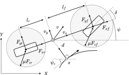
3.1 Vehicle model

Figure 3.1: Illustration of the bicycle model showing the relation between Global X-Y frame and Frenet frame. s denotes the progress along the cen-terline of the lane

3.1.1 Frenet frame

The Frenet frame is an alternate coordinate system to the Cartesian system, that simplifies the representation of a system moving along a continuous and differentiable curve in three-dimensional Euclidean space, by the use of vari-ables s and d, shown in Figure 3.1. s represents the distance traveled along the curve and d represents the perpendicular distance to the curve. Using the frenet frame to describe the vehicle motion along the road centerline makes it possible to formulate the optimization problem for racing by maximizing pro-gression along s while staying inside max and min values of d. All parameters measured as part of the perception system are passed in terms of global X-Y coordinates and is transformed to the local frenet frame, this permits the car dynamics to be described relative to the centerline.

3.1.2 Bicycle model

The vehicle is modeled by representing left and right wheels at the front and rear axles, as single wheels at each of the axle centers. This model is valid by the assumption that the roll dynamics on the left are canceled out by those on the right. This way of modeling a car is called a bicycle model. Equal steering angle for both left and right wheel is assumed, however, this is not always

(30)

CHAPTER 3. THEORETICAL BACKGROUND 14

the case. Although, in general, these angles will be approximately equal [27]. The bicycle model has previously been used in the field of autonomous driving [28], [29], [1], [6], and has become a standard of sorts.

The representation of a bicycle model driving in a track is shown in Figure 3.1. denotes the steering angle, while and c denote the vehicle heading angle

and the angle of path tangent at s measured relative the X-axis, respectively. v is the vehicle velocity, and distance from the center of gravity (CG) to the front and rear axles are given by lf and lr. Lateral forces are denoted as Fyfand Fyr,

longitudinal forces represented as Fxf and Fxr, and rear-wheel is denoted by

the subscript r, while the front wheel is denoted by f. The coordinates of the vehicle are represented in both the traditional X-Y system and the frenet frame.

3.1.3 Dynamic model

Experiments as part of this thesis were conducted using dynamic vehicle mod-els. Consider the dynamic bicycle model represented in Figure 3.1, the vehicle orientation relative to the centerline tangent at s is given as

= c (3.1)

whereby the vehicle dynamics can be described using the frenet frame as ˙s = vxcos( ) vysin( ) 1 dc (3.2a) ˙ d = vxsin( ) + vycos( ) (3.2b) ˙ = ˙ c vxcos( ) vysin( ) 1 dc (3.2c) ¨ = 1 Iz (lfFyf lrFyr) (3.2d) ˙vx = 1 m(Fxf + Fxr Dav 2 x) (3.2e) ˙vy = 1 m(Fyf + Fyr) vx ˙ (3.2f) where ˙ , vxand vydenotes yaw rate, longitudinal velocity and lateral velocity,

mand Izrepresent the mass and moment of inertia of the vehicle and cis the

curvature of the centerline at s. The term vx ˙ represents the centripetal

(31)

Note that the road is flat during this work, therefore bank angle and inclination of the road are assumed to be zero. State and control vectors are selected as

x = [s, d, , ˙ , vx, vy] (3.3)

and

u = [Fyf, Fxf, Fxr]T (3.4)

which allows the state space equation with the control and state vectors can be written as

˙x = f (x, u) (3.5)

Slip Angle

The lateral force on the wheel depends on the characteristics of the tire like the deflection of the treads in the contact between road and wheel. As a result the lateral force on a tire is proportional to the slip angle, when the slip angle is small[27]. Hence, in order to model the lateral force acting on the rear wheel, the slip angle needs to be defined.

Figure 3.2: An illustration of the velocity vector (represented by the red arrow) and the angle relative the rear wheel

The vehicle slip angle is given by

↵r= ✓r (3.6)

where ↵ris the slip angle at the rear wheel and ✓ris the angle of the velocity

vector at the rear wheel, shown in Figure 3.2. The direction of the velocity vector at the rear wheel can be described as

✓r= arctan(

vy lr ˙

vx

(32)

The variation of lateral tire force with slip angle is shown in the figure below.

Figure 3.3: Lateral tire force as a function of slip angle for different road con-ditions. [30]

As seen in Figure 3.3 for small slip angles, the lateral force is proportional to the slip angle [27], if small slip angles are assumed the lateral force can be described as

Fy = C↵↵ (3.8)

where C↵is the cornering stiffness of the wheel. Given equations (3.6),(3.7)

and (3.8), the lateral force on the rear wheels is described as Fyr = 2C↵Fzarctan(

lr ˙ vy

vx

) (3.9)

a factor 2 is included to account for both tires.

Force constraints

The longitudinal and lateral tire forces Fyf, Fxf and Fxf, and the relation

be-tween slip angles and tire forces exist as previously seen. Since these are used as the control parameters, basic Newtonian mechanics is sufficient to get the upper bound to set constraints on these control parameters. Upper bound for the horizontal force acting on the front and rear wheels are given by

Fi  µFzi, i2 [f, r] (3.10) with Fi = q F2 xi+ Fyi2 (3.11)

(33)

f and r stands for front respectively rear wheels, Fzi represents the normal

force on each of the wheels, and µ is the tire-road friction coefficient. The con-dition in (3.11) provides a boundary called the friction circle since it forms a circle with radii µFzi, this is illustrated by the circles around the tires in figure

3.1. Both µ and Fziis dynamically changing with time, the friction varies as a

result of the vehicle driving on different surfaces and Fziis dependent on the

vehicle’s longitudinal acceleration. In order to adapt to changes in the friction, a friction estimation algorithm needs to be implemented to predict the condi-tions ahead of the vehicle. For the purpose of this project, the estimation of the friction will be given by the simulation environment for the models using friction estimation, models without friction estimation will take an assumed value µafor the friction coefficient.

Figure 3.4: Force distribution - side view [27]

The time-varying axle loads can be modeled by moment balance about the two contact points, seen in Figure 3.4, gives the normal forces Fzf and Fzr at the

front and rear wheels as

Fzf = 1 lf + lr (mglr) (3.12) Fzr = 1 lf + lr (mglf) (3.13)

and gives maximum value on Fzi for the models without pitch dynamics and

(34)

trans-CHAPTER 3. THEORETICAL BACKGROUND 18

fer at high accelerations the following relationships are used to calculate the normal force on the front and rear axles taking into account the longitudinal load transfer effects

Fzf = 1 lf + lr (m ˙vxh mghsin✓ + mglrcos✓) (3.14) Fzr = 1 lf + lr ( m ˙vxh + mghsin✓ + mglfcos✓) (3.15)

and sets the maximum value on Fzifor the models with pitch dynamics.

3.2 Optimisation based planning

The thesis utilizes the optimisation based planning algorithm from paper [1]. Optimisation based motion planning involves solving a Constrained Finite Time Optimal Control Problem (CFTOC), at each planning iteration in a re-ceding horizon manner [31] [1]. The friction variation, motion planning CFTOC problem, is as follows: min u0|t,..,uN 1|t J(x_k|t, u_k|t) = p(x_N|t) + N 1_X k=0 q(x_k|t, u_k|t) (3.16) such that, xk+1|t = f (xk|t, uk|t) u_k|t _{2 U}_k|t xk|t 2 Xk|t 8k = 0, ...., N 1 x0|t = xt, xN|t 2 Xk|t

[u_0|t, ...., u_{N 1|t}]T is the input applied to vehicle model f, to generate N+1

states [x0|t, ...., uN|t]T. Functions p(·) and q(·,·) denote the positive definite

running cost and terminal costs respectively. J(·) represents the overall quadratic cost function. Each of the dynamic vehicle models as discussed earlier has its’ own set of states x and inputs u. The predicted trajectory is written as Tt =

(x_x|t, u_k|t), k_{2 (0, ...., N). The predicted states are real at each step and} repre-sents collision free paths for the vehicle to follow. T⇤

t = (x⇤k|t, u⇤k|t, k2 (0, ..., N)).

3.2.1 RTI algorithm

A common method of solving the previously defined optimisation problem in real-time is Real Time Iteration Sequential Quadratic programming (RTI). In

(35)

RTI, an initial guess is obtained from Tt and dynamics are linearised by the

solution obtained from the previous iteration T⇤

t 1. Finally, the state and input

constraints are expressed as linear inequalities. The solution is unsolvable in cases when T⇤

t 1is infeasible and not optimal, at

iteration step t and this leads to some drawbacks of RTI. Unsolvable optimi-sation problem points to the lack of a control signal Uk|tat this iteration step.

The optimal solution from previous time iteration T⇤

t 1 may not be collision

free due to a dynamic environment. RTI algorithm is prone to local sensitivity as it involves discrete decision making (e.g, whether to go left or right of an obstacle) and at rapid changes to the problem constraint (relevant for traction adaption).

3.2.2 sampling augmented real time iteration (SAARTI)

SAARTI overcomes the above mentioned drawbacks of RTI, by the introduc-tion of sampling. SAARTI solves the quadratic cost funcintroduc-tion using the same planning horizon N and discretization step Ts[1], the cost function is described

as

J(xk|t, uk|t) = xTN|tQNxN|t+ N 1_X

k=0

xTk|tQxk|t+ uTk|TRuk|t (3.17)

with QN > 0, Q > 0, and R > 0, representing the tuning matrices. A

dynamically feasible initial guess is generated from T⇤

t 1, by projecting onto

current time step Uk|tand forward integration of dynamics. Additional guesses

created from trajectory rollout [32]. The best guess is selected by evaluating the constraints and the cost function. The QP is then formulated around the initial guess and solved with the constraints. The process is repeated with closed loop control. The algorithm is summarised in the figure below,

(36)

(37)

Implementation

The implementation utilized for batch simulations and setup of experiments is described in this chapter. The initial sections deal with the reasoning for choosing the different parameter configurations and the latter end of the chap-ter deals with the implementation.

4.1 Experimental Setup

4.1.1 Selection of cases

Different track sections that affected the planning performance were identi-fied. Adaption of friction and pitch dynamics were hypothesised to permit better vehicle handling in cornering at higher speeds. U and S sections of track provided a way of testing the vehicle handling under extreme cornering conditions with different complexities. U-section in real races, would start typically with a long straight stretch to accelerate, followed by quick corner-ing and then some acceleratcorner-ing stretch to follow up. S-section, is similar to U-section, except that it has two back to back cornering sections. These sec-tions permit some racing action, given equivalent car and driving parameters, and hence are of interest. S- curve, formed by means of consecutive U turns, was opportune to investigate, if there were any problems due to build up of errors from earlier sections of the track and reasons for parameters like model complexity and planning horizon, affecting it. The effect of planning horizon on the performance and the effect of different models on the physical limits of speed, were tested by the use of tracks of different radii, for both U- and S-sections. The tracks used for testing is shown in Figure 4.1

(38)

CHAPTER 4. IMPLEMENTATION 22

(a) S-shape (b) U-shape

Figure 4.1: The S- and U- curves with different radius which form the cases of the case study, the radius of the curves is denoted as r

4.1.2 Selection of input parameters

The performance of TA, FA, and LA were evaluated individually and also com-pared with a generic model, to conclude how the added dynamics contributed to the performance. NA provided a baseline for performance measurement, which is a widely used vehicle model in the research field. Simulations were done for the different models, using equivalent parameter sets to ensure a fair trial for comparison of results on common grounds.

By identifying different sources of variations the input parameters of inter-est and the levels of variation needed were defined. The purpose was to find what input parameters affected the performance of the path planner. Param-eters were selected in considerations of previous research and the models of interest. Previous work has shown that the planning horizon has an impact on the planning performance[6], and using standard deviation of the tire-road friction coefficient was chosen to study the effect of the friction estimation. The standard deviation values was used to generate friction values for differ-ent parts of the track by draw random samples from a normal distribution. Some questions that were investigated at this stage was, what is the maximum and minimum value, and what step size should be used to ensure that interest-ing behavior isn’t missed. The possible levels of variations are also limited by the number of simulations that were possible to achieve under the restricted time frame.

Values for the planning horizon was decided by running test simulations for TA. The planning horizon denoted as N is the number of states to be generated by the planner. Figure 4.2 shows the failure for TA using different planning horizons and the blue patch represents a 68% confidence interval of failure.

(39)

At the horizon N equal to 30, a sudden increase of the failure can be observed, and running simulations with a failure of 100% would not generate any useful data to analyze. Therefore, the maximum value of N was set to 30. At N equal to 15 a small increase in failure is observed and is therefore chosen as the min-imum value of N. The difference between consecutive N values decided to be five, to capture the entire bandwidth of values between the upper and lower bounds while ensuring a feasible number of simulations.

Figure 4.2: Failure for different N values using TA

NA was hypothesized to be most affected by changes in the tire-road friction coefficient. Hence, the values of the standard deviation of the road friction coefficient, denoted as µ-sd, was selected by running simulations for NA. The variation of the friction coefficient as the car progresses along the track is shown in Figure 4.7. Figure 4.3 shows difference in failure for the chosen values on µ-sd.

Figure 4.3: Effect on NA when varying µ-sd

The failure for tracks with friction coefficient deviation of 0.2 is close to zero and low enough to see a good performance for NA. The failure increases as

(40)

the variance increases at a value of 0.6 a distinct increase in failure was ob-served and about 40%. To limit the number of parameter configurations while observing interesting behavior and ensure timely completion, the variances in friction values were fixed to 0.2 and 0.6.

The models being compared and the cases consisting of the tracks is also in-put parameters to the system. A table of the selected Inin-put variables and their levels of variations is shown in Table 4.1

Model µ-sd N Curve radius Non adaptive (NA) 0.2 15 S 10 Friction adaptive (FA) 0.6 20 U 15 Load adaptive (LA) 25 20 Traction adaptive (TA) 30

Table 4.1: Table showing the input variables and their levels

We evaluated the effect of these input parameters on the planning performance by simulating all combinations of these parameter sets. In total 32 sets of pa-rameters, combinations are simulated for each case in terms of the tracks to explore the effect by individual and combination of parameters, on the plan-ning performance. For each set of parameters, 80 laps were computed.

4.1.3 Identifying Experimental units

Experimental units define the conditions of the environment which decide the conclusions. The number of samples Nsin the planning algorithms using

sam-pling, assumption of tire-road friction coefficient µaused by models without

friction estimation, and sample time Ts were identified as the experimental

units. These parameters were set to give each model as good conditions as possible, to make a fair comparison. µawas set to the mean value of µ for the

whole track, while Ns was set by testing to find a value giving good

perfor-mance. Tsdecides how often planning of a new trajectory is done and was set

to the same value used by [1] and is the same for all models. The values of the experimental units are seen in Table 4.2

µa Ns Ts[ms]

1.6 50 100

(41)

4.1.4 Noise factors

Noise factors are factors that are not considered in the result but affect the re-sult. When running simulations one noise factor identified was the placement of different µ values, meaning if a low value is placed in a sharp corner the risk of failing is higher than if the value was higher. Another factor was the initial conditions on speed and vehicle placement on the road. An important part of the research was to find the different generalisations possible from testing on specific sections. Therefore noise factors were dealt with by introducing randomness into the experiments and running batch simulations, meaning the result is based on the mean values of several laps for each set of parameters. This ensured that the various possible scenarios are accounted for and the most likely output was obtained. Hence permitted the results to be generalised for most sections of the track and answer the research question.

4.1.5 Measurements

The laptime and planning time was measured to conclude performance for dif-ferent models. Data collection and output visualization were integrated into the simulation environment to get an agile understanding of the relations be-tween various parameters.

4.2 Software

4.2.1 ROS

ROS [33] was chosen for handling the functionality aspect of the simulations due to simplicity and modularity. Robot Operating System (ROS) is a middle-ware platform that provides libraries and tools that help softmiddle-ware developers create robot applications. It simplifies the integration of different components on the same system and over the network. A basic ROS system consists of a master, nodes, topics, services, and actions. ROS nodes are executables, that that can exchange information through topics, services, or actions. ROS master ensures that all the nodes are running smoothly and asynchronously. ROS handles the communication of different nodes to run the package as a single system. The entire setup is modular and permits different modules to be swapped in or out. The system of simulation is also close to reality, hence reduce setup time when switching to hardware implementation.

(42)

4.2.2 FSSIM

FSSIM was chosen as the racing simulator. FSSIM is a vehicle simulator ded-icated for Formula Student Driverless Competition. It was developed for au-tonomous software testing purposes. A version of this simulator was used to predict laptime of gotthard car at the Formula student Germany 2018 track-drive competition with one percent accuracy[3]. The simulator allows agile real-time visualisation of closely modeled (to reality) cars to be run on tracks defined by cones. The simulation is run in Gazebo environment with the RVIZ package, on ROS.

4.2.3 ACADO Toolkit

The ACADO toolkit was chosen for handling the real-time optimisation of the different variables while planning the path. ACADO Toolkit is a software environment and algorithm collection for automatic control and dynamic opti-mization. It provides a general framework for using a variety of algorithms for direct optimal control, including model predictive control, state and parameter estimation and robust optimization. The toolkit has an object oriented design, hence permits for easy modifications and optimisations.

4.3 Hardware in the loop

Jetson TX2 is a microcontroller and is used as a standard for hardware im-plementation in the industry. Jetson TX2 has a powerful GPU with parallel computing capabilities, and support for multiple hardware and software ap-plications. This makes it widely used in the field of autonomous driving and robotics. We utilize the Jetson for implementation of the planning algorithm, as the main purpose is to evaluate the planning performance. The other as-pects of the simulation like the racing track and it’s associated parameters are implemented on another host machine, and this mimics the real scenario. The host communicates over ethernet with the Jetson via SSH. Ethernet is used to minimize the communication delay between the different nodes. The control node for the car runs on the Jetson.

(43)

Figure 4.4: Hardware in the loop setup for batch simulations

4.4 System architecture

The simulation was implemented with the system architecture as shown in Figure 4.5. The simulation handler is responsible for handling the entire sim-ulation and is the master node. Simsim-ulation handler is also responsible for re-setting the simulations in case of failure. Experiments need to be run with a different combination of parameters and this is given as input from the up-date ROS parameters node. This node publishes the different input parameters to run the simulation. Run simulation runs one iteration of simulations, this could be single or multiple laps, depending on the input configuration for a single combination of parameters. Experiment manager receives inputs from various nodes like perception, state estimation, and planning, to give output commands to the control interface. The commands to the control interface tell the car how it should be driven in the track. The track, the car and its motion are visualized using RVIZ, figure . The FSSIM node provides the state of the car as feedback for both the experiment manager and planning nodes. The planning node takes input from the previous state of the car and the sample set from sampling augmentation, calculates the optimal path by using differ-ently weighted parameters and constraints, and finally, output path is given to the experiment manager. Planning node runs on the Jetson, while the remain-ing nodes run remotely, allowremain-ing the plannremain-ing performance to be evaluated as independently as possible on actual hardware.

(44)

Figure 4.5: System architecture

Figure 4.6: Visualisation of the planned path and the sample trajectories using RVIZ

4.5 Simulation environment

The visualization of the simulation environment is seen in figure 4.6. The sampled trajectories and the planned path are seen as the blue dotted curves. The speed of the car and the friction estimate is displayed on the screen as the car progresses along the track.

(45)

4.5.1 Obstacles at beginning of race

Racing dictates that the car travels the maximum distance in a minimum time interval and we are interested in randomizing the initial conditions only. Ob-stacles were introduced at the beginning of the race at random locations for each lap, to randomize the initial conditions and ensure a representative sam-ple for analysis. The obstacles appear at a location such that it is far from the start point and also gets sufficient distance to accelerate after passing the ob-stacle, before entering critical testing regions of the race track. The existing architecture permitted running multiple laps continuously while in the results only data for the critical section of the track were considered.

4.5.2 Randomising µ throughout the track

Testing the traction adaptive planning algorithm required varying friction through-out the track. This was achieved by variable friction coefficients at different sections of the track. The coefficients were modeled as a normal distribution function with a mean and standard deviation. The simulations were run with constant mean value and standard deviations of 0.2 and 0.6, a visualization of the varying friction can be seen in 4.7. The coefficients for the Pacejka Tire Model [19] used to calculate the cornering stiffness C↵ in the

simula-tion environment were experimentally identified for a fricsimula-tion coefficient of 1.6[3]. Hence, the mean value of the friction was set to 1.6. The values were randomly generated while following the probability distribution function. The randomly generated values were assigned to smaller sections of the track. This later permitted testing the effect of different models and friction variations.

(46)

(a) µ-sd of 0.2 (b) µ-sd of 0.6

Figure 4.7: A visualization of an s-shaped track with varying friction sections. The colorbar in the bottom shows the colormapping for the friction coefficient sections in the track

4.5.3 Tracks

Critical sections of the tracks in racing include sections with roundabout turns, quick sharp corners, and consecutive corners after long stretches of acceler-ation. The tracks needed to be modeled to permit these sections to be tested while allowing us to run a large number of simulations. Generalisation of the results formed a large part of the test environment and simulations to answer the research question. It was decided to keep the majority of the track a con-stant while only swapping the critical sections to be tested. This would ensure that the results would be due to the critical sections of the track. Sufficient acceleration lengths were provided to ensure the car was going into the curves at high speed and test the adaptability of the algorithm. Tracks generated in frenet frame to allow the car to follow the curve path s and variations along the width represented by d.

4.5.4 Tuning weights for optimisation

The weights of the cost function were tuned to give good performance in rac-ing. A tune process was done where the weights are tuned one after the other. The weights were increased/decreased as long as laptime was consistent or

(47)

decreasing. When the failure or laptime increased the previous value of the weight was used and then the next weight was tuned. This process was re-peated for all weights until the tuning was not changing the weights. Many sets of weights gave good results since the setup is insensitive to tuning, there-fore a large step size could be used when tuning and the same weights could be used for all models.

4.6 Data Post-processing

Extensive experimentation with the different parameter combinations resulted in large data sets and required systematic methods for analysis and visuali-sation. The data is saved as numpy files, with all the details about path tra-versed, path planned, planning samples, vehicle parameters, track parameters, and any other parameter that required investigating. Python pandas were used for collecting all the data and storing the parameters that required investiga-tion. Sometimes failed runs occurred due to factors outside the planner (the object of evaluation) and was filtered out during post-processing.

(48)

Chapter 5 Results and Discussion

During this thesis, it was hypothesized that models with dynamic constraints would perform better than the one with the static constraints up to the point of failure where all computational resources are used. By varying the input parameters that were expected to have the most effect on performance, we evaluate the effect of these parameters on the planning performance for dif-ferent models. Suitable input parameters include the planning horizon and the friction coefficient variance. To generalize the evaluation, the algorithm was tested on several S and U shaped tracks and curves of varying radii. The resulting trade-offs between model complexity and planning horizon and the consequences of variation of input parameters are presented in this chapter. Data gathered by performing batch simulations of 80 laps for each of the com-binations of input parameters which resulted in a total number of 15360 laps. We utilize NA as the baseline for evaluating the planning performance. A single lap on an S-track with low variance on the friction coefficient is plotted in Figure 5.1 for different planning horizons. The vertical color bar represents the variation in speed and the path traced by the car is plotted with the same color coding. Variation in friction coefficient along the track is represented by the colors in the horizontal bar. The four N values represent the planning horizon for each lap. It can be seen that NA manages to plan feasible trajec-tories to compensate for the curve and handles small errors between assumed and real value on the friction coefficient for different planning horizons.

(49)

Figure 5.1: A sample of succeeded laps for NA on an S shaped track with radii= 20 and µ-sd = 0.2. Color mapping on the vehicle path shows the longitudinal velocity in m/s and color mapping on the track shows the real tire-road friction coefficient µ, NA uses an values of µ = 1.6 for planning The following Overview section provides a generic view of the results obtained for all models. To study the effect different input parameters have on planning performance the result is then presented for varying planning horizon, friction variance, and track shapes in separate sections. The effect each of these pa-rameters on output is presented as a contrast between using models with static constraints and models with dynamic constraints. A table of the mean results for all track shapes can be seen in appendix A.

5.1 Overview

This section presents the results and analysis of the data obtained by running 80 laps for each combination of input parameters. The input parameters used is summarized in Table 4.1 from earlier section. To get an overall view of the differences in performance for different models, plots in Figure 5.2, shows how the interaction between models and planning horizon affects failure and lap-time. Results for all track shapes and µ-sd values are combined and visualized by mean value and 68% confidence interval of laptime and failure.

(50)

CHAPTER 5. RESULTS AND DISCUSSION 34

(a) Failure

(b) Laptimes

Figure 5.2: Plots showing failure and laptime vs planning horizon N. Lines illustrate mean value to combine the results for all input parameters and the colored area around the lines illustrates the 68% confidence interval for on each value of N

As seen in Figure 5.2, TA and FA have the lowest failure for planning horizons lower than 25 while NA allows for a higher planning horizon. For a planning horizon of 30, NA has the lowest failure, although it is higher compared to the adaptive models when using lower N. LA was hypothesized to have a higher failure and lower laptime compared to FA and TA, the figure shows that the results are in agreement with this hypothesis. Figure 5.2 shows that FA and TA are close in performance except for a planning horizon of 20, where TA has lower failure and laptime. TA and FA, show the most consistent result in failure which is shown by the shaded area around the curves in Figure 5.2a. The areas for NA and LA is both wider, and LA has lower spread for planning horizons between 20 and 25.

(51)

Table 5.1: Table presenting results at point of failure for each model, the result is an average for all track shapes and radius

Avg. Laptime [s] Failure [%]

Model N µ-sd

Friction adaptive 25 0.2_0.6 _10.729.96 0.00_7.50

Load adaptive 25 0.2_0.6 _10.109.69 _22.920.00

Non adaptive 30 0.2_0.6 9.60_9.69 _24.380.62

Traction adaptive 25 0.2_0.6 _10.899.77 0.21_6.67

The results for all input parameters combined shows that TA has the best per-formance until a certain planning horizon. In the following sections the impact of planning horizon, varying friction coefficient and track shape will be further investigated, to better understand what influences the results seen in Figure 5.2.

5.2 Effect of planning horizon

The planning horizon limits the number of steps to which the car plans ahead in time. Higher planning horizons require higher numbers of computations, while a lower horizon meaning, the car sees a shorter length of the track to follow. Given this, it was hypothesised that all models will first get decreased failure with higher planning horizons and that there will be a trade off when the planning time gets close to point of failure, and failure will start increase with higher planning horizons. Since NA is a less complex model, it is assumed to be less affected by the increased planning time. Consider Figure 5.3 showing laptime and failure for each model.