Fast Estimation of Aggregated Results of Many
Load Flow Solutions in Electric Traction
Systems
L. Abrahamsson, L. S¨oder
Electric Power Systems, Royal Institute of Technology (KTH), Sweden
Abstract
Transports on rail are increasing and major railway infrastructure investments are expected. An important part of this infrastructure is the railway power supply sys-tem. The future railway power demands are naturally not known for certain. This means investment planning for an uncertain future. The more remote the uncertain future, the greater the amount of scenarios that have to be considered. Large num-bers of scenarios make time demanding (some tens of minutes, each) simulations less attractive and simplifications more so. The aim of this paper is to present a fast approximator that uses aggregated traction system information as inputs and out-puts. This facilitates studies of many future railway power system loading scenar-ios, combined with different power system configurations, for investment planning analysis. Since the electrical and mechanical relations governing an electric trac-tion system are quite intricate, an approximator based on neural networks (NN), is applied. This paper presents a design suggestion for a NN estimating power system caused limits on active and reactive power load, i.e., limits on the levels of train traffic.
Keywords: railway, neural networks, load flow.
1 Introduction
For environmental and economic reasons, in Sweden and the rest of Europe, both personal and goods transports on rail are increasing. Therefore major railway in-frastructure investments are expected. An important part of this inin-frastructure is the railway power supply system.
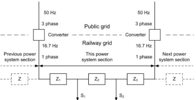
One phase low frequency AC railway power supply systems are normally con-nected to the normal 50 Hz power system through frequency converters, see Figure 1.
Z1 Z2 Z3 S1 50 Hz S2 16.7 Hz 3 phase 1 phase Converter 50 Hz 16.7 Hz 3 phase 1 phase Converter Z Z Previous power system section Next power system section This power system section Public grid Railway grid
Figure 1: A section of the railway power supply system, illustrated as an electric circuit.
The converters may be merely used as power sources, as in Sweden for example, whereas in other countries the railway administrations produce electricity on their own and sell it on the market when profitable. The catenary (the overhead con-tact line from which the locomotive extract electric power) has a relatively high impedance, i.e., the railway power grid normally can be considered weak. The weakness can be somewhat reduced by strengthening the catenary system, plac-ing the converter stations closer to each other, or connectplac-ing a High Voltage (HV) transmission line in parallel to the catenary system. One important consequence of a weak railway power supply system is that when traffic is dense, fast, and/or the trains are heavy, the voltage will drop. For voltages lower than nominal, the locomotives cannot extract as much tractive force as is normally the case. This means that, depending on the strength of the power system, there is a limit on the intensity of the train traffic, caused by voltage drops in the catenary that reduces the maximal tractive force.
Railway power supply systems are changing all the time. When a train moves, the impedances between it and the feeding points changes, because both catenary and HV line impedances are distance dependent. The magnitude of the apparent power demands also change when the trains move. Both the active and reactive power demands of the locomotives may vary with the slopes of the railway, the train weights, the desired train velocity, etc.
When considering future possible railway power supply system investments, for each possible expansion alternative, many different situations of railway operation causing different loading on the railway power supply system have to be stud-ied. This is a kind of transmission expansion planning. Similar approaches can be found in the references [1, 2, 3]. In the case of the railway, however, the locations of feeding points are up to the railway power grid administrator, and not to the
actors on the market as in the case with the public grid.
For each possible investment alternative, the power grid calculations have to be performed fast. There are several algorithms available, e.g., TPSS (Train Power System Simulator, called TTS in [4]) and commercial programs such as TracFeed Simulation [5]. These are however not fast enough, though, when several thou-sands of cases have to be studied. The intention of this paper is to propose a solu-tion of how to design an approximator that rapidly estimates the properties of an electric railway power supply system which are considered important in the stud-ies of future expansion alternatives. In other words, to calculate aggregated results from many load flow calculations in a fast way.
The two most important consequences of train traffic related to the state of the power system, having the railway operation costs in mind, are:
• The power consumption of the grid, preferably divided up by individual converter stations.
• The impact of catenary voltages on the minimal traveling times.
In this paper, the power system impact on travel time limits is studied, and there-fore these are modeled to be the outputs of the approximator. In order to keep the approximator relatively simple, inputs as well as outputs must contain aggregated information. These aggregated figures can, from the power system point of view, be divided into three groups: issues having influence on the power consumed (in-puts), issues having influence on the impedances (in(in-puts), and issues related to voltage drops (outputs). For more details, see sections 3.2.1 and 3.2.2.
Since the electrical and mechanical relations of an electric traction system are quite intricate, an approximator of the black box kind is a tempting approach. Therefore, Neural Networks (NN), which basically are a kind of nonlinear pre-dictors, were selected as a suitable approximator type. One reason to use aggre-gated inputs is that NNs with too many inputs and outputs may need a tremendous amount of training cases in order to become reliable and general [6]. The exact details of the approximation can be studied in section 3.
In a numerical example, an X km section of a traction power supply system is modeled, see section 3.2. The operation is then simulated and the parameters and the performance of the approximator are then estimated. The notation X signifies that the inter-converter distance is varied.
1.1 Related Work
Efforts constructing less complicated approximators, based on knowledge, intu-ition, and experience have been made in [7], an interesting German paper from 1998. That paper presents an obviously very fast and uncomplicated method of approximating impacts of different levels of traffic and different power system setups, on the train speeds. The models in [7] do, however not consider the im-pacts of: slopes, non-maximal train velocities, train velocity and catenary voltage dependencies of the reactive power consumption (which implicitly is done in the model proposed here, from now on called TPSA (Train Power System Approxi-mator) since the approximator is trained with simulation results based on load flow
calculations), different train types at the same railway section, etc.
2 Basic Power System Modeling
2.1 Converters
Traction systems fed through converters, are normally either low frequency one-phase AC systems, or DC systems. A section of the low frequency railway power supply systems used in Northern Europe can be modeled as in Figure 1. Because of the relative weakness of such systems, converters can more or less be consid-ered as power injectors from strong grids. Thereby, converter stations need to be distributed along the railway such that power does not have to be transmitted over too great distances, and such that the converters do not get overloaded.
The frequency converter stations in Sweden control their terminal voltages, al-though not stiffly. The voltage is controlled linearly with respect to reactive power generation. Converter stations can produce reactive power of both positive and negative signs. If no reactive power is generated, the catenary voltage is controlled at a nominal level (16.5 kV). The voltage angles at the converter station terminals are completely determined (although quite nonlinearly) by the voltage levels, and the active and reactive power flows in and out of the terminals of the converter station.
In Figure 1, the power system sections are fed from both ends. In reality, how-ever, a railway power system section can also be supplied only from one side. Singly fed sections are not studied in this paper, but can for example occur at cate-nary ends, or in cases of converter outages.
2.2 Power Transmission
The impedances Zj, j ∈ {1, 2, 3}, in Figure 1, denote the total impedances as
seen by the locomotives. Included in these impedances one can find catenary impedances as well as (if present) impedances originating from the high voltage lines and the transformers connecting them to the catenary.
The impedance values do not only depend on the train positions (impedances are normally length dependent), they also depend on the power system configuration. Basically, there are two kinds of catenary technologies used: Booster Transformer (BT) and Auto Transformer (AT). BT is the cheaper one, with higher impedances than AT [8]. There is also an option of strengthening the power system by installing a High Voltage (HV) transmission line in parallel to the catenary. The impedances between the locomotives and the converter stations are naturally smaller, the more densely the transformers connecting catenary and HV line are distributed.
2.3 Locomotives and Trains
For a train to move forward, a tractive force is needed, depending on its running resistance (mainly air and mechanical resistance), its weight, the locomotive’s
ef-ficiency, and track topography, different force levels are needed for acceleration or speed maintenance. Moreover, depending on the train velocity, the catenary volt-age levels, and possible additional controls, the tractive force outtakes are bounded. The following is important, especially from the power system dimensioning viewpoint. For sinking catenary voltage levels, for a constant amount of consumed power, the currents tend to increase. Therefore the tractive force is successively reduced by on-locomotive controllers. This control is installed in order to protect the engine from overloading. The connection between tractive force, F , and the electric active power consumed, P , is, P = F · v, excluding electrical and me-chanical losses in the train, and where v denotes train velocity. Thus, in weaker traction power systems, if the traffic demand is too high, the trains will be forced to travel either more sparsely, more slowly, or a combination of the two, compared to what would be the case if the power system had an unlimited capacity. An im-portant difference between locomotives and other kinds of power consumers is that locomotives to a greater extent accept substantial voltage drops. Thus, even a typical Swedish locomotive will still be in operation, at a reduced level of tractive force, for voltage drops of about 40 %. The electrical and mechanical rules of train movements are described in some detail in [4, 9].
Summarizing the preceding paragraph, trains are movable and heavily varying electric power loads. In the exemplifying circuit of Figure 1, the apparent power consumed by the two trains Si= Pi+ jQi, i∈ {1, 2} can be found. As indicated
in the above, the apparent power is not constant with respect to time and position. For some (older) locomotive types, the reactive power consumption, Qi, depends
on catenary voltage levels, Pi, and v, see e.g. [4, 9] for details. For more modern
locomotive types, Qican be controlled freely but such locomotives are, at least in
Sweden, normally operated purely resistively [10].
3 The Approximator
3.1 Introduction
The aim of the approximator (TPSA), is to obtain a fast estimation of whether a certain power system causes limitations in possible train power consumption levels, i.e., in possible train traffic.
Since the voltages are almost stiff at the catenary side of the converter station terminals, the railway power supply system can be divided into separate sections by using the converters as section borders. These sections are almost independent of each other. This means that train traffic on one side of a converter station in-fluences the catenary voltage levels on the other side of that particular converter station to a comparatively small extent. The power flows between these power sys-tem sections are normally insignificant, but the smaller the impedances, the more noticeable they are.
In [11], one modeling simplification is that a train consumes power only from the feeder units right in front of and right behind it. There, ”feeder unit” means either a converter station or a transformer station connecting the catenary to the
transmission line.
With this assumption, the inputs to TPSA, as well as the outputs from it, only have to describe the traffic and power system states for one section at the time. The power system sectioning assumption is an essential part of the TPSA model presented here. The fact that the TPSS simulations for the creation of the TPSA training set will treat smaller power systems, and thereby further reduce the simu-lation times, must simply be considered as a bonus. The main benefit considering future usage of TPSA is that it will now become a general module that can be used for any traction power system section in a greater system. The part of TPSA that determines the maximal on-average velocities can be used as traffic-dependent constraints in a suitable time table program. Such a constraint states the maximal on-average velocity for an additional train, given an already existing traffic.
The main difference between the TPSA model presented in this paper, and the so called TTSA in [4] is that inputs and outputs are aggregated differently. In this paper the choices of aggregation are better adjusted for the kind of information that one can expect to be available. In [4], the active power consumption of the railway was also estimated. Since this paper is more detailed, all focus is here set on the impacts of minimal train running times as a function of the strength and the load of the power supply system.
3.2 The Model
It is common in train time table planning programs to use models containing binary or integer variables for train location. The models vary, but are similar. From now on, assume we have a binary variable, say xi,j,ti,tj,r, that takes on the value1 when there is traffic on that particular railway section in that particular time window with that particular train, and equals0 when not. The indices designate the following: i is the node (a node in a traffic planning model, i.e., a train stop) from which the train leaves at time ti, j is the node at which the train will arrive at time tj, whereas
r is the train index.
The facts explained above regarding train timetable planning are crucial for the modeling of TPSA, i.e., the choices of the aggregated inputs and outputs for the TPSA. The inputs and outputs of TPSA must be such that they are possible to aggregate both from TPSS as well as time tabling programs.
The points in time when the studied (additional) train starts, ti, and stops, tj, are
crucial when aggregating the inputs and outputs. For example they make it possible to know when to start measuring the behavior of the other trains (connected to the same power system section as the studied train during the time interval between ti
and tj). Obviously, all trains are limited by the catenary voltage levels, but TPSA
is designed such that each train is studied at a time. Separate TPSA:s for different numbers of trains on the power system sections would make the approximator less general and probably demand a greater set of training data.
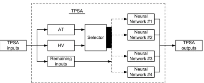
The choices of important aggregated TPSA inputs and outputs are in the bullet lists of sections 3.2.1 and 3.2.2 described and motivated. The binary variables AT and HV describing the power system technology are not aggregated, and as shown
in Figure 2 even not really inputs to the NN, and therefore not found in the bullet list of section 3.2.1.
3.2.1 The Aggregation of Inputs
The TPSA inputs can be classified as either parameters giving rise to the con-sumption of active and reactive power, or parameters related to the power system impedances. Some inputs may be connected to both consumption and impedance. In this paper, the trains are allowed to stop only at the locations of converter stations, a fact that reduces the number of input variables. Additionally, the model is restricted to one type of trains traveling in one direction. The TPSA inputs of this paper can be found in the following bullet list, including short motivations.
• The distance between i and j, denote it d (i, j). The distance gives informa-tion of the power system impedances.
• The average inclination, E (incl), between the power system section-borders i and j. The average inclination gives information of the net potential energy consumed by the trains. The other trains will not experience the same incli-nations as the train studied in the time interval between tiand tjdoes.
• The standard deviation of the inclination, D (incl), between the power sys-tem section-borders. The average inclination, E(incl), would for example equal zero for both flat ground as well as for a rail section with 20 per mille uphill half the section and 20 per mille downhill the remaining half. The standard deviation is a measure of how much the inclinations fluctuate, which will influence the consumed electric power of the trains.
• The traffic of other trains on the studied power system section in the time interval between tiand tj must also be measured, because within that time
interval, the power consumed by ”other trains” affects the catenary voltages experienced by the ”studied” train. The average velocity, E(v), and the aver-age number of trains, E(trains), on the section are calculated. The velocity is used because higher train speeds means greater power consumption. The average velocity is measured only when trains are in service. The number of trains is important because the more trains, the greater need for electricity. The average number of trains is calculated as total train traffic time divided by the length of the time window, tj− ti.
3.2.2 The Aggregation of Outputs
The TPSA output describes the running times influenced by catenary voltage levels for the studied train.
• The fastest possible average velocity of the studied (added) train.
3.2.3 Neural Network
The output of TPSA is the greatest possible average speed for an added train. The inputs of TPSA describe the power system topology and parameters, the topogra-phy of the track, and the number of other trains (on the same power system section as the studied train) as well their average speeds. TPSA is essentially a NN that connects the inputs to the outputs.
TPSA inputs AT HV Remaining inputs Neural Network #2 Neural Network #1 Neural Network #3 Neural Network #4 Selector TPSA TPSA outputs
Figure 2: For AT and BT catenary types, who can be either connected to or with-out an HV transmission line, there are four separate possible neural net-works.
Moreover, some of the TPSA inputs describing the power system are binary, i.e., AT , which equals1 for AT catenaries and equals 0 for BT catenaries, and HV , which indicates the presence of HV transmission lines when it equals1. Two binary variables give four possible combinations. For each of the four cases, an individual NN is constructed, see Figure 2. The separation into four different NNs is motivated by the fact that backpropagation [12, 13] networks are not optimal for such classifications [6]. Backpropagation networks are mainly approximators of smooth functions. Thus, the NNs are only trained with inputs and outputs that can be regarded as continuous variables, i.e., ”remaining inputs” in Figure 2.
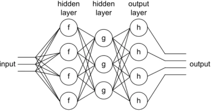
Two different NN models are proposed, both based on the assumed outputs and inputs presented in sections 3.2.1 and 3.2.2. An example of a multilayered neural network can be found illustrated in Figure 3. In that network, there are three layers, of which two are hidden. Normally, all neurons in one layer have the same type of transfer functions, e.g., f in the first layer in Figure 3.
The first model, M1, is a nonlinear NN with two layers. In M 1, the hidden layer hastanh transfer functions,
out1n = tanh b 1 n+ 5 X k=1 inkw 1 k,n ! (1)
where subscript n denotes neuron number and superscript1 denotes the first layer. The input vector is, as can be deduced from the bullet list, of length5 and the output is just a scalar. The second (output) layer has a linear transfer function
out2= b2 + N X n=1 out1nw 2 n (2)
where superscript2 denotes the second layer, and N is the number of neurons in the first layer. The parameters b1
n, b 2
, w1
k,n, and w 2
n are parameters whose values
are determined in the training step. According to the theory, page 78 in [14], and in [13], this kind of network can be used as a general function approximator, given a sufficient amount of neurons in the hidden layer.
f f f f input g g g h h h h output hidden layer hidden layer output layer
Figure 3: A sketch of an arbitrary neural network. The input vector is three ele-ments long, whereas the output vector is four eleele-ments long.
The second model, M2, assumes a linear dependency
out= b +
5
X
k=1
inkwk (3)
where k is input index, and wk and b are parameters whose values are determined
in the training process presented in section 3.2.3.1.
The motivation for testing a linear model at all is explained by the planned future use of TPSA as a running time constraint in a train time tabling program. In such a program, time consuming already as it is, a linear model would probably not extend the computation times as much as a nonlinear one would. The accuracies of the two models are compared and evaluated in section 4.2.
3.2.3.1 Training of the Neural Network In both models, i.e., M1 and M 2, the aggregated input and output data sets are normalized to lie in the interval[−1, 1] before training and testing the approximators.
Training is essentially a method of determining the values of the parameters w and b (in both M1 and M 2), such that the mean square of the estimation error of the network output is minimized.
Model M1 is trained by thetrainbr(Bayesian regularization
backpropaga-tion) algorithm (of Matlab’s NN Toolbox) with an error goal of10−5. Thus, out2
of equation 2 is the estimation of the maximal train velocity.
Model M2 is trained by thetrainb(batch learning) algorithm (of Matlab’s
NN Toolbox). Thus, out of equation 3 is the estimation of the maximal train ve-locity.
4 Numerical Example
4.1 Problem Setup
In order to be as clear a possible, in the numerical example presented in this paper, just a few of all possible parameters are presented and used. That makes the prob-lem setup more surveyable. For example, only one kind of trains is studied (simi-larly as in [4]), only one kind of each respective catenary type is studied, unidirec-tional traffic is assumed, and the converter stations are all assumed to be equipped with six 10 MVA converters (Q48/Q49) each such that the installed power should not be a limiting factor in the simulations studied. Furthermore, the train stops are also assumed to coincide with the locations of the power system section borders, i.e., the converter stations. The speed limit is set as high as 150 km/h all over the simulated railway sections, i.e., for Rc4 locomotives a limiting constraint only in very steep downhill situations. Moreover, the number of transformers connecting the transmission line (when present) to the catenary is set to three in all cases stud-ied in this paper. The model presented in section 3.2 is as simple as it is in order to comply with these model restrictions. All trains also try to go as fast as possible in the TPSS simulations, excluding a lot of real-life cases.
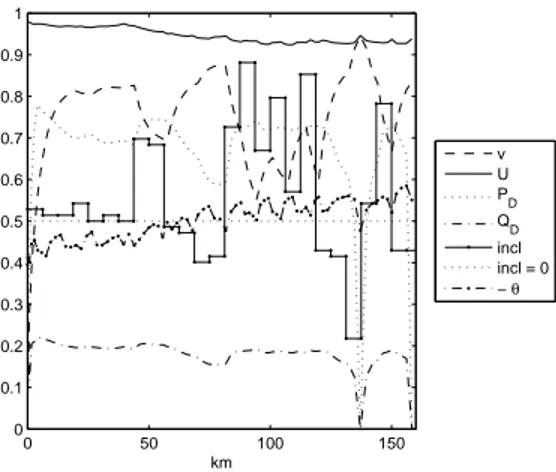
In Figure 4, a train from a TPSS simulation is studied. In that simulation, the converter distance was 160 km on an AT system with HV line and the train de-parture periodicity was 6 minutes. The velocity of the train, v, is scaled down by a factor of160 km/h. Additionally, the figure presents the consumed active power, PD, reactive power, QD, and the catenary voltage, U , all expressed in p.u., where
Sb = 5 MVA and Ub = 16.5 kV. The catenary phase angles of opposite sign, i.e,
−θ, seen by the locomotive of the train can also be found in Figure 4, expressed in radians. Finally, the inclinations of the railway track are also plotted in Figure 4, scaled such that0 on the y-axis means −10 per mille, and 1 means 10 per mille.
In the numerical example, 400 different simulations have been done, 100 for each neural network to train. There are four separate NNs, one for BT catenaries, one for AT catenaries, one for BT with transmission line, and finally one for AT with transmission line – as described in Figure 2.
These hundred cases consists of ten different inter converter distances (of length: 30, 57, 80, 98, 114, 127, 138, 146, 154, and 160 km) combined with ten different train departure periodicities (of times: 6, 8, 10, 13, 17, 22, 28, 36, 46, and 60 minutes between each train departure).
In the numerical example of [4], the measuring of a train’s running time is not started until the railway is filled up with trains according to a certain train departure periodicity. In this study, in order to speed up the calculations, the measuring is started immediately. In order not to have a completely empty railway when starting measuring, in the initialization procedure, TPSS distributes trains along the track almost as in an ideal situation, i.e., trains going at maximally allowed speed all the time. After the simulation has started, however, of course the trains distributed along the track with predefined initial velocities will follow the same electrical and mechanical laws of nature as the other trains.
0 50 100 150 0 0.1 0.2 0.3 0.4 0.5 0.6 0.7 0.8 0.9 1 km v U P D Q D incl incl = 0 − θ
Figure 4: An example of the mechanical and electrical states of a train traveling through a section of the railway electric power supply system.
4.2 Numerical Results
The greatest on-average velocity, for an added train, is determined through TPSS simulations with the problem setup presented in section 4.1.
Worth pointing out is that all simulations use the same railway profile, e.g., the first 30 km in all simulated cases have the same inclinations. Consequently, the average values and standard deviations of the inclinations will be different for each inter-converter distance.
As rule of thumb [6], two thirds of the simulations may be used for training the NN, whereas the remaining third may be used for testing. That is applied also here. The amount of hidden neurons, i.e., N in equation 2 was set to4. This was not done arbitrarily, but by studying the average (ten different random choices of training and testing sets) mean square approximation errors for one to ten hidden neurons – see Figure 5.
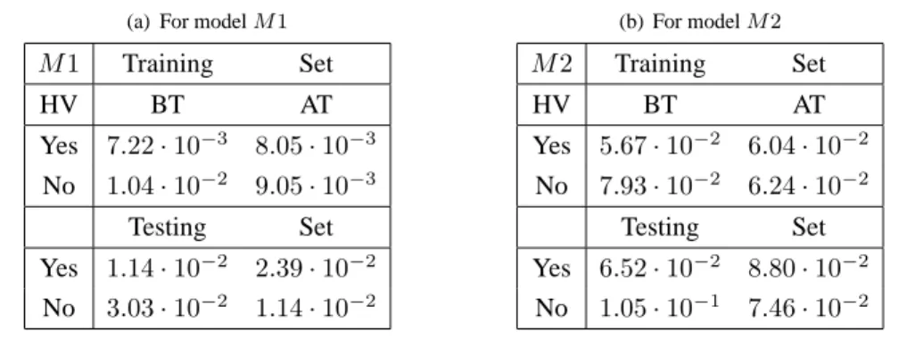
In the case studies, the accuracies of one linear NN and one nonlinear NN are compared for both the training and the testing sets. The approximation errors in Table 1(a) can be found for network M1, and Table 1(b) for network M 2. The NNs are modeled with the design introduced in section 3. The computer time needed for execution of minor NNs like these is negligible.
5 Conclusion and Summary
The paper can be concluded with the fact that a first suggestion to a fast method of estimating the fastest possible train speeds, for an additional train, as a function of the railway power supply system and the traffic level of other already added trains. The function uses aggregated parametric values as both inputs and outputs.
1 2 3 4 5 6 7 8 9 10 0.01 0.02 0.03 0.04 0.05 0.06 0.07 0.08 0.09 0.1 0.11
Number of neurons in hidden layer
Average Mean Square Error
Training Set Test Set
Figure 5: A study of the average mean square errors on the training and testing sets as a function of the amount of hidden neurons.
Table 1: The approximation errors for the four different neural networks (a) For model M 1
M1 Training Set HV BT AT Yes 7.22 · 10−3 8.05 · 10−3 No 1.04 · 10−2 9.05 · 10−3 Testing Set Yes 1.14 · 10−2 2.39 · 10−2 No 3.03 · 10−2 1.14 · 10−2 (b) For model M 2 M2 Training Set HV BT AT Yes 5.67 · 10−2 6.04 · 10−2 No 7.93 · 10−2 6.24 · 10−2 Testing Set Yes 6.52 · 10−2 8.80 · 10−2 No 1.05 · 10−1 7.46 · 10−2
In the numerical example, an example of the results of TPSS were presented in a graph. That is followed up with a comparison between the two suggested
approx-imator models M1 and M 2. As one could expect, the non-linear model performs
noticeably better.
Some recommendations for further work:
• Include different traveling directions in the model • Include trains with different speed limits
• Allow train stops at arbitrary locations • Include different train types
• The next step of TPSA: estimate the injected active power, and the dividing up between the converter stations.
References
[1] Cruz-Rodrgues, R.D. & Latorre-Bayona, G., HIPER: Interactive Tool for Mid-Term Transmission Planning in a Deregulated Environment. Power En-gineering Review, IEEE, 20(11), pp. 61–62, 2000.
[2] Buygi, M.O., Balzer, G., Shanechi, H.M. & Shahidehpour, M., Market-Based Transmission Expansion Planning. Power Systems, IEEE Transactions on,
19(4), pp. 2060–2067, 2004.
[3] Chennapragada, B., Radhakrishna, C. & Vallampati, R., Risk-based approach for Transmission Expansion Planning in Deregulated Environment. Prob-abilistic Methods Applied to Power Systems, 2006. PMAPS 2006. Interna-tional Conference on, Stockholm, Sweden, 1–4.
[4] Abrahamsson, L. & S¨oder, L., Fast Calculation of the Dimensioning Factors of the Railway Power Supply System. Computational Methods and Experi-mental Measurements, Prague, The Czech Republic, volume XIII, pp. 85–96, 2007.
[5] Stern, J., TracFeed Simulation, Reference Manual. Technical Report BBSE951112-BNA, Balfour Beatty Rail, 2006.
[6] Communication with Bj¨orn Levin, SICS - Swedish Institute of Computer Science, 2007. Kista, Sweden.
[7] v Lingen, J. & Schmidt, P., Railway Electric Energy Supply and Operation of Railways (original title in German). Elektrische Bahnen, 96(1–2), pp. 15–23, 1998.
[8] B¨ulund, A., Deutschmann, P. & Lindahl, B., Circuit design of the Swedish railway Banverket in catenary network (original title in German). Elektrische Bahnen, 102(4), pp. 184–194, 2004.
[9] Abrahamsson, L. & S¨oder, L., Basic Modeling for Electric Traction Systems under Uncertainty. Universities Power Engineering Conference, 2006. UPEC ’06. Proceedings of the 41st International, Newcastle upon Tyne, UK, vol-ume 1, pp. 252–256, 2006.
[10] Communication with A. B¨ulund, Swedish national railway administration (Banverket), 2007. Borlnge, Sweden.
[11] Nyman, A., TTS/SIMON Power Log – a simulation tool for evaluating elec-trical train power supply systems. Computers in Railways VI, Lisbon, Portu-gal, 1998.
[12] Backpropagation. http://en.wikipedia.org/wiki/
Backpropagation, 2007.
[13] Neural Network Toolbox (Matlab online help). www.mathworks.com/
access/helpdesk/help/toolbox/nnet/backpro4.html.
Re-trieved on March 9 2007.