2007:29 Intercomparison of Cement Solid-Solution Models

Research

SKI Report 2007:29

Intercomparison of Cement Solid-Solution

Models

Issues Affecting the Geochemical Evolution of

Repositories for Radioactive Waste

Steven Benbow

Colin Walker

David Savage

May 2007

SKI Perspective

Background

Many concepts for the geological storage of radioactive waste incorporate cement based materials, which act to provide a chemical barrier, impede groundwater flow or provide structural integrity of the underground structures. Thus, it is important to understand the long-term behaviour of these materials when modelling scenarios for the potential release and migration of radionuclides. In the presence of invasive groundwater, the chemical and physical properties of cement, such as its pH buffering capacity, resistance to flow, and its mechanical properties, are expected to evolve with time.

Purpose

The purpose of this study is to address the uncertainty regarding the choice of model for the CSH (calcium-silicate-hydrate) gel dissolution. One small scale and one large scale model from work performed during 2005 is taken as base case and the cement model is replaced with two other cement models recently developed by other researchers. The results are compared to the last years modelling to give an estimate of the model uncertainties.

Results

Two alternative CSH solid solution aqueous solution (SSAS) models are compared with the one that was used in the earlier work, with an emphasis on a direct comparison of the model predictions.

The results suggest that the three models are generally in agreement regarding the degradation of CSH gel and the overall cement and therefore that the modelling results of the previous report would be largely unaffected if an alternative cement model were used. One of the alternate CSH SSAS models considered is notably different from the others in its underlying assumptions (Sugiyama and Fujita). It assumes different end-member solids, which may make it applicable to the modelling of low pH cements, which are being considered in the context of HLW repositories in order to avoid some of the possible deleterious interactions between high pH cement waters and other EBS materials.

Continued activity in the research area

Further studies are needed to evaluate which model(s) are applicable to use for modelling the degradation of low pH cements.

Effect on SKI supervisory and regulatory task

An understanding of the behaviour and influence of cement in repositories is necessary for upcoming SKI reviews of SKB reporting for repositories for low- and intermediate level waste (SFR) and spent nuclear fuel. This study will a constitute a basis for further dialogue with SKB on the use of cement in repositories and on the required knowledge base for new materials.

Project information

Responsible at SKI has been Christina Lilja SKI reference: SKI 2006/366

Project number: 200609032

Earlier reports in this project: Benbow, S., Watson, C., and Savage, D., Investigating conceptual models for physical property couplings in solid solution models of cement, SKI Report 2005:64, Swedish Nuclear Power Inspectorate, Stockholm, November 2005.

Research

SKI Report 2007:29

Intercomparison of Cement Solid-Solution

Models

Issues Affecting the Geochemical Evolution of

Repositories for Radioactive Waste

Steven Benbow

1

Colin Walker

2

David Savage

1 1

_{Quintessa Ltd.}

The Hub

14 Station Road

Henley-on-Thames

United Kingdom

2

_{Department of Mineralogy}

The Natural History Museum

Cromwell Road

London

SW7 5BD

United Kingdom

May 2007

This report concerns a study which has been conducted for the Swedish Nuclear Power Inspectorate (SKI). The conclusions and viewpoints presented in the report are those of the author/authors and do not

Contents

Summary ... 1

1. Introduction ... 3

2. Thermodynamics background... 5

2.1. General thermodynamics... 5

2.2. Thermodynamics of solid solutions... 8

2.3. The model of Börjesson et al. (1997) ... 10

2.4. The model of Walker (2003) ... 13

2.5. Summary of Börjesson et al. and Walker’s thermodynamic data ... 15

2.6. The model of Sugiyama and Fujita (2005)... 16

2.7. Comparing Ca(OH)2 activity predicted by the solid solution models ... 19

3. Numerical simulations... 21 3.1. Concrete composition ... 22 3.2. Secondary minerals... 24 3.3. Rates of reaction ... 25 3.4. Fluids ... 28 4. Results... 31 5. Conclusions... 35 References... 37

Summary

Many concepts for the geological storage of radioactive waste incorporate cement based materials, which act to provide a chemical barrier, impede groundwater flow or provide structural integrity of the underground structures. Thus, it is important to understand the long-term behaviour of these materials when modelling scenarios for the potential release and migration of radionuclides. In the presence of invasive groundwater, the chemical and physical properties of cement, such as its pH buffering capacity, resistance to flow, and its mechanical properties, are expected to evolve with time.

Modelling the degradation of cement is complicated by the fact that the long term pH buffer is controlled by the incongruent dissolution behaviour of calcium-silicate-hydrate (C-S-H) gel. It has been previously shown (SKI Report 2005:64) that it is possible to simulate the long term evolution of both the physical and chemical properties of cement based materials in an invasive groundwater using a fully coupled geochemical transport model. The description of the incongruent dissolution of C-S-H gel was based on a binary solid solution aqueous solution (SSAS) between end-member components portlandite (Ca(OH)2) and a C-S-H gel composition expressed by its component oxides

(CaH2SiO4). The models considered a range of uncertainties including different

groundwater compositions, parameterised couplings between the evolution of porosity with permeability and diffusivity and alternative secondary mineral assemblages. The results of the modelling suggested that alternative evolutions were possible under these different conditions.

The focus of this report is to address the uncertainty regarding the choice of model for the C-S-H gel dissolution. We compare two alternative C-S-H SSAS models with the one that was used in the previous report, with an emphasis on a direct comparison of the model predictions. Thus we have chosen one simple simulated experimental model based on those in the previous report, but with some of the process coupling removed so that the differences between the C-S-H models can be more directly compared.

The results suggest that the three models are generally in agreement regarding the degradation of C-S-H gel and the overall cement and therefore that the modelling results of the previous report would be largely unaffected if an alternative cement model were used. One of the alternate C-S-H SSAS models considered is notably different from the

others in its underlying assumptions (Sugiyama and Fujita). It assumes different end-member solids, which may make it applicable to the modelling of low pH cements, which are being considered in the context of HLW repositories in order to avoid some of the possible deleterious interactions between high pH cement waters and other EBS materials.

1. Introduction

Many concepts for the geological storage of radioactive waste incorporate cement based materials, which act to provide a chemical barrier, impede groundwater flow or provide structural integrity of the underground structures. Thus, it is important to understand the long-term behaviour of these materials when modelling scenarios for the potential release and migration of radionuclides. In the presence of invasive groundwater, the chemical and physical properties of cement, such as its pH buffering capacity, resistance to flow, and its mechanical properties, are expected to evolve with time.

Modelling the degradation of cement is complicated by the fact that the long term pH buffer is controlled by the incongruent dissolution behaviour of calcium-silicate-hydrate (C-S-H) gel. It has been previously shown (Benbow et al., 2005)) that it is possible to simulate the long term evolution of both the physical and chemical properties of cement based materials in an invasive groundwater using a fully coupled geochemical transport model. The description of the incongruent dissolution of C-S-H gel was based on a binary solid solution aqueous solution (SSAS) between end-member components portlandite (Ca(OH)2) and a C-S-H gel composition expressed by its component oxides

(CaH2SiO4). The models considered a range of uncertainties including different

groundwater compositions, parameterised couplings between the evolution of porosity with permeability and diffusivity and alternative secondary mineral assemblages. The results of the modelling suggested that alternative evolutions were possible under these different conditions.

The focus of this report is to address the uncertainty regarding the choice of model for the C-S-H gel dissolution. We compare two alternative C-S-H SSAS models with the one that was used in the previous report, with an emphasis on a direct comparison of the model predictions. Thus we have chosen one simple simulated experimental model based on those in the previous report, but with some of the process coupling removed so that the differences between the C-S-H models can be more directly compared.

The report is structured as follows. In section 2 we describe the thermodynamic theory that forms the basis for the three cement models. We show that the three models have a common background and describe the way in which each model differs from the others. In section 3 we give details of the numerical model that is used in the comparison and in

section 4 we give the results. The key results and conclusions are summarised in Section 5.

2. Thermodynamics background

2.1. General thermodynamics

Thermodynamics is the study of energy and its transformations, which, from a

geochemical viewpoint, can be applied to the equilibrium states of minerals. Generally, we are interested in whether a particular mineral is either dissolving or precipitating, which for a mineral reaction may be simply defined as

mineral. dissolved

mineral

solid ⇔ (2.1)

Using the mineral calcite (CaCO3) as an example, the dissolution reaction can be written

CaCO_{3( s )} = Ca_{( aq )}2+ + CO_{3( aq )}2− .

Whether the mineral should be in the solid state or dissolved state can be determined by considering the change in Gibbs free energy of the reaction, Δ_rG. For any given reaction, there are three conditions of interest (i) when Δ_rG < 0 the dissolution reaction will be spontaneous, (ii) when Δ_rG = 0 the reaction is in equilibrium and at a Gibbs free energy minimum and (iii) Δ_rG > 0 the precipitation reaction will be spontaneous. While it is difficult to measure absolute values of ΔrG, it is standard practise to

calculate the Gibbs free energy of formation for a substance in standard state, Δ_fG0, from the difference between the Gibbs free energy of the substance and the Gibbs free energy of its constituents. The standard state refers to a pure mineral at some

temperature and pressure of interest, typically 25 °C and 1.01325 bar. Again, using calcite as an example, Δ_fG_CaCO

3( s ) 0

can be calculated from

. 5 . 1 0 0 0 0 0 ) ( 2 ) ( 3 ) ( 3s CaCO s Ca C O g CaCO fG =G −G −G − G Δ

Values of Δ_fG0 are tabulated in thermodynamic databases for most common minerals, solids, liquids, gases, and solutes.

Minerals dissolve and precipitate to minimise the magnitude of the Gibbs free energy of the system and bring it to equilibrium. Thus, if we write the reaction as

¦

α_iS_i = ,0 (2.2) where α_i is the stoichiometry of species S in the reaction (note that there is no _i

distinction between the species S being a mineral, solid, liquid, gas or solute), then the _i minimal Gibbs free energy of the reaction in the standard state is written as

. 0 0

¦

Δ = ΔrG αi fGS_i (2.3) The values 0 i S fG

Δ are the differences between the Gibbs free energy of formation of the substances S in standard state and the sum of the Gibbs energies of formation of its i

constituent parts in standard state. Again, considering calcite as an example, Δ_rG_CaCO

3( s ) 0

can be calculated according to

. 0 0 0 0 2 3 2 ) ( 3 ) ( 3 =Δ −Δ + −Δ − ΔrGCaCO s fGCaCO s fG_Ca fG_CO Since values of 0 i S fG

Δ are tabulated in thermodynamic databases for most common minerals, solids, liquids, gases, and solute species, Δ_rG0_{can be determined for most}

reactions of interest.

The activity of a substance, a is defined in terms of the difference between the Gibbs _i free energy of the substance and the Gibbs free energy of the substance in standard state, . ln 0 i i i G RT a G − = (2.4)

This equation is often seen in the form μ_{i −}μ_i0 ₌RT lna_i

, where μ_i is the chemical potential of species i. The chemical potential is essentially the Gibbs energy per mol, so working with μ_i can avoid problems relating to the fact that G varies with the _i concentration of species i if species i is a solute.

If we assume that the constituent parts of the reaction are indivisible (so that

i i fG =G

(

)

(

)

∏

¦

¦

¦

= = − = Δ − Δ = Δ − Δ i i i i i i i i i i i f i f i r r i a RT a RT G G G G G G α α α α ln ln 0 0 0 (2.5) Writing Q to be the ion activity product ( =

∏

i i

i

a

Q α ), and defining the value of Q at equilibrium (when Δ G_r =0) to be K_eq, we have

eq

rG0 =RTlnK

Δ

− , (2.6)

where Keq is defined as the equilibrium constant of the reaction. The values of Keq (or

equivalently _G0

r

Δ ) are tabulated in thermodynamic databases for most reactions of interest. Therefore , ln eq r K Q RT G= Δ (2.7)

and at equilibrium the activity of the aqueous species in solution, defined by the ion activity product Q, should equal the activity of the aqueous species in solution defined by the equilibrium solubility product, Keq, i.e. at equilibrium we have Q=Keq.

Again using calcite as the example, at equilibrium

(

)

(

)

1 2 3 2 2 3 2 = = ⋅ ⋅ − + − + eq m equilibriu CO Ca water CO Ca K Q a a a a

Because Q may vary by orders of magnitude, it is more convenient to take the log of the ratio

eq

K Q

. log

K Q

SI = (2.8)

SI is a form of a free energy of which there are three conditions of interest, which can be related to the direction of the reaction. When (i) SI < 0 the solution is said to be undersaturated and the mineral of interest will dissolve (ii) when SI = 0 the solution is said to be in equilibrium with the mineral of interest and (iii) when SI > 0 the solution is said to be oversaturated and the mineral of interest will precipitate.

2.2. Thermodynamics of solid solutions

Notice that in the previous analysis there was no distinction between the case when the species S was a solid, liquid, gas or solute. In the case of a single pure mineral, the _i activity is usually taken to be 1, so that Q is purely a function of the activity of the solute species (for a suitable choice of porewater basis species).

Now, if we consider a solid solution mineral composed of two or more end-members, denoted S_j, then the chemical potential of each end-member can be written as

, ln 0 j j j =μ +RT a μ (2.9)

where aj is the activity of end-member j . The activity of the end-member in a solid

solution is given by , j j j X a = γ (2.10)

where X_j is the mol fraction of end-member j in the solid solution and γ is the solid _j phase activity coefficient.

For the solid solution reaction, we can then write in terms of Gibbs free energies

(

0

)

, 0 j f j f j j r rG −Δ G = X Δ G −Δ G Δ

_¦

_(2.11)

. ln 0 j j j r rG −Δ G =

¦

X RT a Δ _(2.12)

Now, since Δ_rG0 can be expressed as

( )

¸ ¸ ¹ · ¨ ¨ © § −

∏

j X j j K

RTln 0 , using (2.10) we have that

. ln ln ln 0 _j j j j j j j j j rG =−RT

¦

X K +RT

¦

X X +RT

¦

X γ Δ _(2.13)

We now restrict attention to the case when there are two end-members; a binary solid solution. In both the Börjesson et al. (1997) and Walker (2003) models (sections 2.3 and 2.4), the two end-members are taken to be portlandite (Ca(OH)2) and a C-S-H gel

(CaH2SiO4). CaH2SiO4 is an empirical formula representing the simplest stoichiometry

of a C-S-H gel expressed by its component oxides. In the Sugiyama and Fujita (2005) model (section 2.6) the end-members are taken to be Ca(OH)2 and SiO2(s).

Both Börjesson et al. (1997) and Walker (2003) base their approach to modelling solid solutions by providing a method of determining the solid phase activity coefficients in this equation, however the approach taken in determining the coefficients is different. Sugiyama and Fujita (2005) base their approach on the “conditional equilibrium

constant”, but it can be related back to determining the solid phase activity coefficients. The final term in (2.13) is referred to as the excess Gibbs free energy of mixing,

. ln excess j j j rG =RT

¦

X γ Δ _(2.14)

If each end-member were treated as an ideal mineral, then its activity coefficient would be 1 and the final term would disappear. Hence the previous equation can be expressed as . excess ideal ideal -non G G G _{r r} r =Δ +Δ Δ (2.15)

Several empirical expressions exist to model the excess energy of the solid solution as a function of the solid solution composition. Most of these are of Margules type, which express the excess energy as a power series of mol fractions (e.g. Glynn, 1991). One

such fitting function is the polynomial suggested by Guggenheim (1937, 1952), referred to as the Guggenheim mixing model,

(

)

¦

= − = Δ n k k k rG X X A X X 0 2 1 2 1 excess . (2.16)

Here, the A are coefficients that are independent of the solid solution composition but _k can depend on temperature and pressure.

Both the Börjesson et al. and Walker models use the Guggenheim mixing model as the basis for the determination of the solid phase activity coefficients of each end-member. What distinguishes each model is the way in which the Guggenheim mixing model is parameterised. This is described in the following two sections.

2.3. The model of Börjesson et al. (1997)

In Börjesson et al. (1997), the two end-members are taken to be portlandite (Ca(OH)2)

and a C-S-H gel (CaH2SiO4) with end-member reactions

( )

O. 2H SiO Ca 2H SiO CaH O, 2H Ca 2H OH Ca 2 2(aq) 2 4(s) 2 2 2 2(s) + + = + + = + + + + +

The Guggenheim polynomial (2.16) is truncated after two terms to obtain the sub-regular Guggenheim expression

(

)

[

_{0 1 1 2}

]

. 2 1 excess X X A A X X G r = + − Δ (2.17)

Next, the following expression (due to Prausnitz, 1969) is used to express the solid phase activity coefficient of an end-member as a function of Gexcess,

(

)

. ln n G_excess n RT _{T r} j j Δ ∂ ∂ = γ (2.18)

Here n_j is the number of moles of end-member j , and n is the total number of moles _T of the solid solution. This expression is then evaluated for the first end-member (taken to be Ca(OH)2),

(

)

[

3

]

, ... ₂2 _{0 1 1 2} 2 1 2 1 1 0 2 1 2 1 1 X X A A X n n n n A A n n n n n ¸¸_¹= = + − · ¨ ¨ © § » ¼ º « ¬ ª + − + + ∂ ∂ (2.19) to obtain

(

)

[

0 1 1 2

]

2 2 1 3 ln X A A X X RT γ = + − . (2.20)

The saturation index of the end-members is defined as

, log ₀ j j j K Q SI = _(2.21) and so . 10 0 j SI j j j j j K Q a X = = = γ (2.22)

Börjesson et al. (1997) use data from the literature (Kalousek, 1952) to evaluate

2 Ca(OH)

SI at various Ca/Si ratios of the solid phase(s). This is then used to fit A and ₀ A₁ to complete the formula forγ₁, the activity coefficient of Ca(OH)2 . The fitted values of

0

A and A were found to be ₁

-1 0 =3.26kJmol

A and A₁ =13.44kJmol-1.

The same A and ₀ A values are then used to define ₁ γ₂, the activity coefficient of CaH2SiO4, using

(

)

[

3

]

, ... ln 2 _{0 1 1 2} 1 2 X A A X X RT γ = = + − (2.23)

The Ca(OH)2 data is therefore essentially used to fit both end-members, although this is

not unreasonable given the much more soluble Ca(OH)2 end-member has such a strong

influence on the solubility of the system.

This allows Börjesson et al. to calculate solid phase activity coefficients for each end-member as a function of the mol fractions of the end-end-members in the solid solution. Then it is possible to calculate Q /_j K_j to determine the direction of each end-member reaction individually.

As presented above, the model over-predicts the activity of Ca(OH)2 for calcium-rich

C-S-H gels. Following Glasser et al. (1987), Börjesson et al. postulate the existence of a miscibility gap for Ca(OH)2 mole fractions greater than 0.3 (corresponding to a Ca/Si

ratio 1.43), when the C-S-H gel may in fact exist as two solid solutions with one being close to pure Ca(OH)2. Since the Ca(OH)2 end-member then co-exists almost as a pure

mineral, the activity of Ca(OH)2 is capped at unity for Ca/Si ratios greater than 1.43.

This is shown in Figure 2.1.

0 0.5 1 1.5 2 2.5 3 0.5 1 1.5 2 2.5 3 C/S ratio P o rt la n d ite a c ti v ity

Not fixed for Ca-rich Fixed for Ca-rich

Notes on the Börjesson et al. (1997) model

Since the composition of the C-S-H gel end-member CaH2SiO4 has Ca/Si = 1, the

model is only relevant to C-S-H gel in cement systems with Ca/Si • 1. This makes the model less applicable to low pH cement systems.

2.4. The model of Walker (2003)

Walker (2003) similarly takes the two end-members in the solid solution to be portlandite (Ca(OH)2) and a C-S-H gel (CaH2SiO4), but derives values for the

Guggenheim parameters A and ₀ A (section 2.3) using miscibility gap data. The ₁ miscibility gap is defined as a compositional range where two phases coexist, typically expressed as mole fraction of the more soluble end-member. In this case, these are (i) a C-S-H gel – Ca(OH)2 solid solution phase and (ii) the more soluble end-member

Ca(OH)2. The miscibility gap will be denoted either

[

X1L,X1U

]

or

[

X2L,X2U

]

(where i

i X

X₁ =1− ₂ ), where the first interval denotes the range of mol fractions of Ca(OH)2 for

which the minerals are miscible and the second interval denotes the corresponding range of CaH2SiO4.

The Guggenheim parameters can be related to the miscibility gap intervals, in terms of mole fraction of Ca(OH)2, using expressions (2.20) and (2.23) for the activity

coefficient of each end-member. It is useful to rearrange these equations as

(

)

[

0 1 2

]

2 2 1 3 4 ln X A A X RT γ = + − ,

(

)

[

4 3

]

ln ₂ = X₁2 A₀ +A₁ X₁ − RT γ . (2.24)

Writing γ_1L, γ_1U, γ_2L and γ_2U for the activity coefficients of each end-member evaluated at the upper and lower bounds of the miscibility gap, and using similar subscripts for the mole fractions of the end-members evaluated at the same points, it follows that

(

)

(

(

) (

3

)

)

2 3 2 2 2 2 2 1 2 2 2 2 0 1 1 _{3 4} ln _{U L U L U L} L U _{A X X A X X X X} RT = − + − − − γ γ _. (2.25) Hence

(

)

(

(

) (

)

)

¿ ¾ ½ ¯ ® ­ _{− + − − −} = = 3 2 3 2 2 2 2 2 1 2 2 2 2 0 1 1 1 1 1 1 1 1 _{exp 3 4} L U L U L U L U L U L U L U _{X X X X} RT A X X RT A X X a a X X γ γ _.

Here a_1U and a_1L are the activities of the first end-member (taken to be Ca(OH)2)

evaluated at the upper and lower bounds of the miscibility gap. However, outside the miscibility gap, these activities are 1, hence

(

)

(

(

) (

)

)

¿ ¾ ½ ¯ ® ­ _{− + − − −} = 3 2 3 2 2 2 2 2 1 2 2 2 2 0 1 1 _{exp 3 4} L U L U L U U L _{X X X X} RT A X X RT A X X . (2.26)

For the other end-member, CaH2SiO4 , a similar relationship holds,

(

)

(

(

) (

)

)

¿ ¾ ½ ¯ ® ­ _{− − − − −} = 3 1 3 1 2 1 2 1 1 2 1 2 1 0 2 2 _{exp 3 4} L U L U L U U L _{X X X X} RT A X X RT A X X . (2.27)

Entering the miscibility gap bounds in the above two equations and solving for the values of A and ₀ A then allows the Guggenheim mixing model to be parameterised ₁ using only the miscibility gap data. However, although the lower miscibility gap compositional boundary was found experimentally by the occurrence of Ca(OH)2 as a

distinct phase (and therefore within the miscibility gap), the upper limit was determined by the best fit of the model prediction to the experimental solubility data of Walker (2003); making the model semi-empirical.

Thus the key difference between the cement model of Börjesson et al. (1997) and that of Walker (2003) is in the derivation of the Guggenheim parameters. As was the case for the Börjesson et al. model, for Ca/Si ratios inside the miscibility gap the Guggenheim polynomial is capped at the value at the lower bound of the miscibility gap. In Walker’s experiments, the miscibility gap was found to be bounded by Ca(OH)2 mole fractions of

0.39 (real) and 0.93 (fitted), which corresponds to Ca/Si ratios of 1.64 and 1.43 (as used by Börjesson et al., section 2.3). The fitted A and ₀ A values were found to be ₁

-1 0 =4.51kJmol

A and -1

1 =2.56kJmol

A .

Notice that in the above approach to relating the miscibility gap bounds to the Guggenheim parameters (which is a recognised approach in the literature, see for example Kersten, 1996) the value of the activity of Ca(OH)2 at the miscibility gap

boundaries is not set equal to one. The mathematical constraints in the derivation simply imply that the activity at each end of the miscibility gap should be the same. Despite this fact, the derived Ca(OH)2 activities in the mode are actually very close to

one as can be seen in Figure 2.2 in section 2.7.

Notes on the Walker (2003) model

Similar to the model of Börjesson et al. (section 2.3), both end-members contain calcium, and so the minimum Ca/Si ratio that the model can be applied to is 1.

2.5.

Summary of Börjesson et al. and Walker’s

thermodynamic data

The parameters in the Guggenheim thermodynamic mixing model and log K (specific) values for each end-member are given in Table 2.1 for the end-member reactions

( )

O. 2H SiO Ca 2H SiO CaH O, 2H Ca 2H OH Ca 2 2(aq) 2 4(s) 2 2 2 2(s) + + = + + = + + + + +

Table 2.1 Thermodynamic data for the Börjesson et al. and Walker models

A0 (kJ/mol) A1 (kJ/mol) 0_{Ca( )OH}

2

K

log logK0CaH2SiO4

Börjesson et al. 3.26 13.44 22.7 15.89

2.6. The model of Sugiyama and Fujita (2005)

Sugiyama and Fujita (2005) take the two end-members in the solid solution to be Ca(OH)2 and SiO2(s). They truncate the Guggenheim polynomial after three terms and

express Δ_rG as , ln lnK₁ RT K₂ RT G r =− − Δ (2.28) in order to write

(

)

(

)

[

]

. ln ln ln ln 2 2 1 2 2 1 1 0 2 1 0 2 1 X X A X X A A RT X X X X K X K K _j j j j j j − + − + − + − = +

_¦

_¦

(2.29)

Sugiyama and Fujita then equate the terms to write

(

)

(

)

[

]

. ln ln ln 2 2 1 2 2 1 1 0 2 1 0 X X A X X A A RT X X X X K X K j j j j j j j j − + − + − + − = , (2.30)

i.e. the excess energy is split into contributions from each end-member, with the contribution from each end-member having the same form as the entire excess energy, so that A_k = A_1k +A_2k. It is in this step that Sugiyama parts company with the solid solution theory in both Börjesson et al. and Walker’s approaches, since Sugiyama and Fujita are effectively expressing the excess Gibbs energy with a modified Guggenheim polynomial that has the form of the sum of two cubic polynomials (multiplied by

2 1X X ):

(

)(

)

¦

= − + = Δ 2 0 2 1 2 1 2 1 excess . k k k k rG X X A A X X (2.31)

Hence the Sugiyama and Fujita model uses six degrees of freedom in their data fit as opposed to two in both the Börjesson et al and Walker models.

, 0 j j j j X K K = γ (2.32)

(i.e. the model allows the equilibrium constants to vary rather than calculating activity coefficients) to derive

(

)

(

)

(

)

(

)

[

]

. ln 1 ln 1 ln 2 2 1 2 2 1 1 0 2 1 0 X X A X X A A RT X X X X K X j j j j j j j j − + − + − + + − − = γ (2.33)

Sugiyama and Fujita then use available solubility data for C-S-H to calculate saturation indices of each end-member at various Ca/Si ratios. They were able to achieve a fit of the three term Guggenheim model to the data to provide a model of γ for each end-_j member. To calculate the fit, Sugiyama and Fujita split the available solubility data into two sets corresponding to data for Ca/Si < 0.833 and Ca/Si >0.833 (0.833 is the Ca/Si ratio of tobermorite; a believed natural analogue of C-S-H gel as found in cement, e.g. Taylor 1997). They then perform a least-squares fit of both sets of data to obtain activity coefficient curves in each Ca/Si region. Furthermore, they argue that for Ca/Si ratios below 0.461 it is appropriate to assume that λ_SiO2 =1 since the solid composition at such low Ca/Si ratios is close to amorphous silica. Similarly for Ca/Si ratios above 1.755, they argue that pure Ca(OH)2 separates from the solid solution and coexists with

C-S-H gel, hence above this limit it is appropriate to treat each end-member separately as an ideal solid.

This approach allows Sugiyama and Fujita to calculate piecewise curves of K_j for each end-member as a function of the mol fractions of the end-members, with reactions as follows:

( )

. SiO SiO O, 2H Ca 2H OH Ca 2(aq) 2(s) 2 2 2(s) = + = + + +

The conditional equilibrium constant curves have the following form:

(

)

(

)

(

) (

)

(

)

[

(

)

(

)

2

]

0 0 2 1 17 . 164 2 1 724 . 36 019 . 37 1 1 log 1 log 1 log log log 461 . 0 / 0 z z z z z z K z K z K K S C C C S S − + − + − + − − − − = = ≤ <

(

)

[

(

)

(

)

]

(

)

(

) (

)

(

)

[

(

)

(

)

2

]

0 2 0 2 1 17 . 164 2 1 724 . 36 019 . 37 1 1 log 1 log 1 log 1 2 241 . 58 1 2 754 . 57 623 . 18 1 log log log 833 . 0 / 461 . 0 z z z z z z K z K z z z z z z K z K S C C C S S − + − + − + − − − − = − − − + − − + − = ≤ <

(

)

[

(

)

(

)

]

(

)

(

) (

)

(

)

[

(

)

(

)

2

]

0 2 0 2 1 792 . 50 2 1 8302 . 7 937 . 36 1 1 log 1 log 1 log 1 2 033 . 25 1 2 712 . 49 656 . 18 1 log log log 755 . 1 / 833 . 7550 . 1 / 833 . 0 z z z z z z K z K z z z z z z K z K S C S C C C S S − − − + − + − − − − = − + − + − − + − = ≤ < ≤ < 81 . 22 log 853 . 7 log / 755 . 1 = − = < C S K K S C where 1 / 1 + = S C z

and 710logKS₀ =−2. is the equilibrium constant for amorphous silica (at 25°C).

Notes on the Sugiyama and Fujita (2005) model

Since Sugiyama’s model considers Ca(OH)2 and SiO2 as end-members in the solid

solution reaction, a wide range of Ca/Si ratios can be modelled. In particular the model could possibly be applied to simulating low pH cements, which typically have a lower Ca/Si ratio in the C-S-H gel.

2.7.

Comparing Ca(OH)

2

activity predicted by the

solid solution models

The Ca(OH)2 activities that are predicted by each of the solid solution models are shown

in Figure 2.2 for a range of Ca/Si ratios. Also marked are the interval boundaries at Ca/Si=0.833 (tobermorite) and Ca/Si=1.755 (Ca(OH)2 co-existence) in the Sugiyama

and Fujita model. Notice that the models of Börjesson et al. and Walker can only be applied to cases where Ca/Si>1 whereas that of Sugiyama and Fujita can be applied to the full range Ca/Si>0 due to the different choice of end-members in the model. Also shown in the figure are some of the data sets that were used to perform the fitting exercises for the models. The Kalousek (1952) data was the primary data source used for fitting Börjesson et al.’s model. The Greenberg and Chang (1965) dataset is one of the four datasets (which included Kalousek’s) that was used to fit the Sugiyama and Fujita model. It should be noted that the Greeberg and Chang data generally gives the lowest activities at Ca/Si>1 of the datasets that were used, hence the poor fit for Ca/Si>1, but is the only dataset that contained measurements for Ca/Si<0.5.

-7 -6 -5 -4 -3 -2 -1 0 1 0 0.2 0.4 0.6 0.8 1 1.2 1.4 1.6 1.8 2 C/S ratio log Ac ti v it y (Ca (O H) 2 ) Sugiyama model Borjesson model Walker Kalousek data Greenberg data

Figure 2.2 Ca(OH)2 activity predicted by each of the solid solution models together

with some of the data used for fitting. Note that Sugiyama’s model is applicable to a wider range of Ca/Si ratios due to the choice of portlandite and SiO2 end-members.

3. Numerical simulations

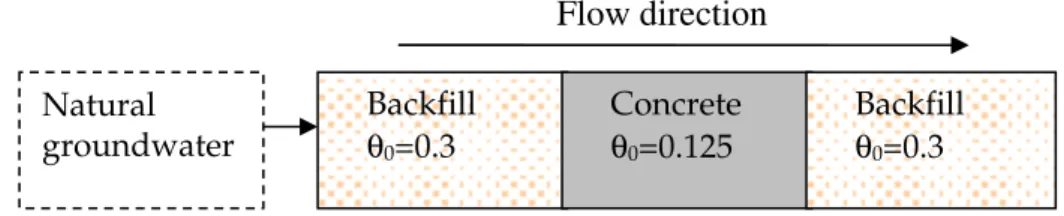
We model the system shown in Figure 3.1 (which is based on models considered in Benbow et al., 2005). The system comprises of a concrete region sandwiched between two backfill regions. The concrete region is composed of cement and a quartz

aggregate with a total porosity of 0.125, and is described in more detail in Section 3.1. The backfill regions are assumed to be composed of crushed quartz particles and have a total porosity of 0.3. Each region in the model is discretised using a number of non-uniformly spaced compartments to more finely capture the behaviour of the model at the interfaces between the regions. At the inlet end of the model, a natural groundwater enters the system. Details of the groundwater are given in Section 3.4.

Transport of aqueous species in the model arises as a result of diffusion and advection. The earlier modelling study (Benbow et al., 2005) considered a variety of possible couplings between the effective diffusivity of the cement and its state of degradation. However in this study, to keep the comparison of the various cement models simple we will take a fixed effective diffusivity of 6×10-10

m2/s in the backfill and 1×10-11 m2/s in the concrete.

Figure 3.1 Schematic of the modelled system

A head gradient is imposed across the system, which gives rise to a flow in the direction indicated in Figure 3.1. The porewater velocity is governed by the head gradient, the hydraulic conductivity and the porosity of the various regions in the model. Head differences are chosen to give rise to models with Darcy velocities of 1, 1×10-2

and 1×10-4

m/y.

In the earlier modelling study (Benbow et al., 2005), the groundwater velocity was fully coupled to the evolving porosity that resulted from the dissolution and precipitation of

Flow direction Backfill θ0=0.3 Concrete θ0=0.125 Backfill θ0=0.3 Natural groundwater

minerals in the system and the permeability of the various regions was coupled to the degree of degradation via the Kozeny-Carmen relationship (see for example, de

Marsily, 1986). In the simulations presented here, the flow velocity is held constant by setting the molar volume of all minerals to zero in the evolution equations. This results in a fixed porosity for all time. Whilst this is physically less realistic, it allows results from the various models to be compared simply without having to account for changes in porosity (in particular we do not need to worry about pore clogging events) and flow velocity. For example, this simplification makes it possible to compare cement

degradation as a function of the volume of water flushed through the various models.

3.1. Concrete composition

The models of Börjesson et al. (1997) and Walker (2003) can both use the same cement composition since they use the same end-members in the description of the C-S-H solid solution model. The cement composition is based upon that in Börjesson et al. (1997). Katoite (Ca3Al2H12O12) and AFm (Ca4Al2SO10) have been chosen to be representative

of the choice of C3AH6 and C4AS H12 by Börjesson et al. (where, in the cement

chemistry nomenclature of Börjesson et al., C=CaO, A=Al2O3, H=H2O and S = SO3).

The cement is used to make concrete with porosity 0.125 (this porosity being representative of the scale from 0.1 to 0.15 quoted in Karlsson et al., 1999). For

modelling purposes, pure quartz particles with a 4 mm diameter and density of 2.65×106

g/m3are used to represent the aggregate components of the concrete. The ratio of cement to quartz by weight is 1:4.4. At this ratio, one m3 of concrete contains approximately 316 kg of Ca(OH)2 and C-S-H, which is in agreement with the rough

estimate of 350 kg of cement per m3 of concrete quoted in (Karlsson et al., 1999), of which approximately 321 kg is composed of Ca(OH)2 and C-S-H. The resulting initial

composition of the intact concrete regions is shown in Table 3.1. For the purposes of the initial volume calculation, the molar volume of CaH2SiO4 was taken to be the sum

of the Ca(OH)2 and quartz molar volumes.

The cement composition used in the Sugiyama and Fujita (2005) model is different due to the different choice of end-members. The amounts of Ca(OH)2 and SiO2(s) have

been chosen to give the same Ca/Si ratio and volume as the cement used in the Börjesson et al. and Walker models, and all other cement amounts are kept the same. For the calculation, the SiO2(s) end-member was assumed to have the same molar

volume as the quartz aggregate.

The backfill regions of the model were taken to be composed entirely of quartz with 30% porosity, as shown in Table 3.3

Table 3.1 Initial cement composition used in Börjesson et al. (1997) and Walker (2003) models

Mineral Initial Concentration

(mol/m3) Molar Volume (cc/mol) Volume Fraction (%) Quartz 30 853.0 22.688 70.0 Ca(OH)2 2 137.0 33.056 7.0 C-S-H 1 175.0 55.744 6.6 Katoite 4.2 149.520 0.06 AFm 137.0 177.000 2.4 Brucite 289.0 24.630 0.7 Porosity 12.5% 12.5

Table 3.2 Initial cement composition used in Sugiyama and Fujita (2005) model

Mineral Initial Concentration

(mol/m3) Molar Volume (cc/mol) Volume Fraction (%) Quartz 30 853.0 22.688 70.0 Ca(OH)2 3 312.0 33.056 10.9 SiO2(s) 1 175.0 22.688 2.7 Katoite 4.2 149.520 0.06 AFm 137.0 177.000 2.4 Brucite 289.0 24.630 0.7 Porosity 12.5% 12.5

Table 3.3 Backfill composition used in all models

Mineral Initial Concentration

(mol/m3) Molar Volume (cc/mol) Volume Fraction (%) Quartz 30 853.0 22.688 70.0 Porosity 30.0% 30.0

3.2. Secondary minerals

The solid products that are considered in the models are subdivided into those that form in the backfill regions of the system and those that can form anywhere (i.e. in the concrete region and the backfill region). This division precludes, for example,

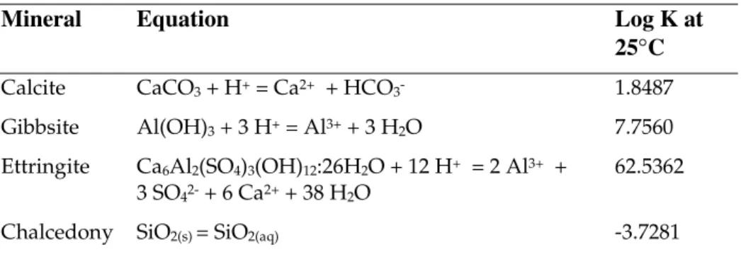
precipitation of the calcium silicate end-member outside the concrete region , since the gel is perceived as a wholly synthetic phase produced only by the hydration of cement clinker. Other secondary phases are mostly calcic phases which could form due to the interaction of groundwater with concrete, e.g. calcite, ettringite. The stable silica polymorph at low temperature is assumed to be chalcedony.

Secondary minerals were allowed to form anywhere in the system (i.e in both the

backfill and concrete regions) and thermodynamic data for these are shown in Table 3.4.

Table 3.4: Thermodynamic data for secondary minerals.

Mineral Equation Log K at

25°C

Calcite CaCO3 + H+ = Ca2+ + HCO3- 1.8487

Gibbsite Al(OH)3 + 3 H+ = Al3+ + 3 H2O 7.7560

Ettringite Ca6Al2(SO4)3(OH)12:26H2O + 12 H+ = 2 Al3+ +

3 SO42- + 6 Ca2+ + 38 H2O

62.5362

Chalcedony SiO2(s)= SiO2(aq) -3.7281

Tobermorite is taken to be representative of all possible secondary C-S-H phases in the system. Thermodynamic data for tobermorite is presented in Table 3.5.

Table 3.5: Thermodynamic data for tobermorite.

Mineral Equation Log K at

25°C Tobermorite-14A Ca5Si6H21O27.5 + 10 H+ = 5 Ca2+ + 6 SiO2(aq) + 15.5 H2O 63.8445

We disallow precipitation of secondary C-S-H phases in the concrete regions to be consistent with the solid solution models, which are all two end-member models and do not consider additional C-S-H phases. Hence, the secondary C-S-H phase will only be permitted to form in the backfill regions.

Over long time periods and higher temperatures (50-100 °C), C-S-H gel might be expected to convert to tobermorite and/or jennite. C-S-H gel could thus be envisaged to both dissolve and recrystallise simultaneously. This recrystallisation of C-S-H into a thermodynamically more stable phase could slow down C-S-H gel dissolution and overall degradation of the cement component of the concrete. Crystallisation of C-S-H gel would however, lead to lower ambient pH values in coexisting groundwater

(Atkinson et al., 1995). This recrystallisation process was studied by Atkinson et al. for an 80°C repository system, but quantitative data regarding the kinetics of this process is unavailable. At lower temperatures, the conversion of C-S-H gel to a more crystalline form will probably be a very slow process and has thus been excluded from model calculations presented here.

3.3. Rates of reaction

The C-S-H gel and portlandite phases were modelled as a SSAS described in sections 2.3, 2.4, and 2.6. Each of these models allows an in-situ activity to be calculated for each of the Ca(OH)2 and C-S-H end-members for the current cement composition.

Using this activity and the porewater composition, the saturation of each end-member can be calculated. Then we can use a Transition State Theory rate equation (e.g. Helgeson et al., 1984) of the form,

¸¸ ¹ · ¨¨ © § − = 1 i i i i i K Q A k dt dC ,

to model the rate of dissolution of each end-member. Here C (mol mi

-3

) is the concentration of end-member i per total volume, ki(mol m

-2

y-1) is the rate of the reaction per surface area of end-member and A (m_i 2 m-3) is the surface area of the end-member per unit volume. Q /_i K_i represents the saturation state of the end-member. We model the solid solution as being essentially instantaneous by choosing k to be _i large compared to the other reaction rates and timescales in the system.

Kinetic models for quartz and calcite are taken from Knauss and Wolery (1988) and Busenberg and Plummer, (1986) respectively. All other minerals in the system are modelled using a fast kinetic rate to approximate instantaneous dissolution and precipitation. The reaction rates can all be characterised as

[ ]

¸¸ ¹ · ¨¨ © § − ¸ ¹ · ¨ © § + 1 K Q a = k A dt dC n H .

Here, C is the concentration of the mineral (mol m-3), kis the rate of the reaction per reactive surface area (mol m-2 y-1), Ais the available reactive surface area (m2 m-3), a_H+

is the activity of the H+ ion in solution and Q/K represents the degree of saturation of the mineral in the fluid phase and n is a nonlinear coefficient that is used to obtain a better fit to experimental data for a range of pH values.

The available surface area, A, is calculated from the mineral concentration in the compartment, C(mol m-3), using

C M S

A= _{SA W} ,

where S_SA is the specific surface area of the mineral (m2 g-1) and M_Wis the molecular weight (g mol-1). This model of available surface area does not take into account any armouring effects when one precipitated mineral covers the surface of another, but is largely irrelevant for fast rates that are approximating an instantaneous precipitation and dissolution assumption (which also ignores armouring effects).

Table 3.6 lists the physical properties of all of the minerals in the simulations. In the calculations in (Benbow et al., 2005), molar volumes were used to calculate porosity changes which are continuously coupled to the evolving flow field calculation. However in these calculations the molar volumes have been assumed to be zero to effectively decouple the flow field and make inter-model comparison more

straightforward between the solid solution models. Molar weight and surface area values are used to derive reactive surface areas from the mineral concentrations in the compartments when calculating kinetic rates of reaction. Surface area data was not available for all minerals, but this is not especially important when fast reaction rates are being used that approximate instantaneous equilibration.

Table 3.6: Mineral physical properties1.

Mineral Molar Volume

(cc/mol) Molar weight (g/mol) Surface area (m2/g) Portlandite 33.056 74.0927 0.02 C-S-H 55.7442 _{134.1769 0.02} SiO2(s) 22.688 60.0843 0.02 Quartz 22.688 60.0843 5.66×10-4 Katoite 149.520 378.2852 0.02 AFm 177.000 634.5462 0.02 Brucite 24.630 58.3197 0.02 Calcite 36.934 100.0872 0.0210 Gibbsite 31.956 78.0036 0.02 Ettringite 715.000 1 255.1072 0.02 Chalcedony 22.688 60.0843 0.02 Tobermorite-14A 286.810 830.0532 2.27 1

Quartz surface area assumes a 4 mm particle with density 2.65×106 g/m3, as in Benbow et al. (2004); calcite surface area from Savage et al. (2002); surface area value of 2.27 m2/g for tobermorite chosen to be the same as in Benbow et al. (2004); all other values chosen to be 0.02. Surface areas are to some extent unnecessary for minerals modelled using very fast kinetic assumptions provided that vastly different surface area values are not assumed.

2

The values of the parameters in the model for the quartz and calcite reactions are given in Table 3.7. The fast kinetic rates to approximate the instantaneous equilibrium assumption for all of the other non-cement minerals each use n=0.

Table 3.7: Reaction rate parameters for quartz and calcite.

k (mol m-2 y-1) n Reference

Quartz 1.58×10-9 _{-0.5 Knauss and Wolery, 1988.}

Calcite 1.99×102 _{0 Busenberg and Plummer, 1986}

The rate of consumption of Ca2+ and OH- from the fluid phase through precipitation of secondary C-S-H (tobermorite) is dependent upon the assumed rate of reaction of quartz and its associated reactive surface area. Here, the experimentally-measured data of Knauss and Wolery (1988) have been used, together with an assumption of sand grain sized quartz particles for surface area calculations. Clearly, any variation of quartz dissolution rate and associated reactive surface area will affect the consumption of Ca2+ and OH- from the fluid phase accordingly.

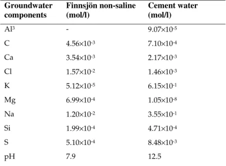
3.4. Fluids

The pore space in the concrete regions is initially occupied with pore water that is equilibrated with respect to the cement. The pore space in the backfill regions is initially filled with the natural host rock pore water that is intruding into the system through the in-flowing boundary. A representative natural host rock water from Karlsson et al. (1999) has been considered: “Finnsjön non-saline”, a high carbonate non-saline water. The composition of each of the porewaters is shown in Table 3.8. A calcium-dominated cement water has been chosen as the initial fluid in the concrete regions to prevent any initial dissolution of the Ca(OH)2 and C-S-H phases. A precise

formulation of the cement water is not especially important since it will be quickly washed out of the system or equilibrated with the cement.

Preliminary modelling showed that the “Finnsjön non-saline” water is saturated with respect to calcite, which leads to calcite clogging the incoming water boundaries in the

model (when porosity was allowed to evolve). Thus the compositions were adjusted to be in equilibrium with calcite.

The aqueous speciation reactions that are included in the models are shown in Table 3.9.

Table 3.8: Groundwater compositions used in the modelling.

Groundwater components Finnsjön non-saline (mol/l) Cement water (mol/l) Al3 _- 9.07×10-5 C 4.56×10-3 7.10×10-4 Ca 3.54×10-3 2.17×10-3 Cl 1.57×10-2 1.46×10-3 K 5.12×10-5 6.15×10-1 Mg 6.99×10-4 1.05×10-8 Na 1.20×10-2 3.55×10-1 Si 1.99×10-4 4.71×10-4 S 5.10×10-4 8.48×10-3 pH 7.9 12.5

Table 3.9: Aqueous speciation reactions included in the models.

Reaction Log K O H H OH + = 2 + − _13.9951 O 4H Al 4H Al(OH) 2 3 4 + = + + + = _22.1400 − + −_{+ =} 3 2 3 H HCO CO 10.3288 O H Ca H CaOH+ ₊ + ₌ 2+ _{+ 2 12.8500} O H Mg H MgOH+ ₊ + ₌ 2+ _{+ 2 11.6820} ( ) H O SiO H HSiO₃− + + = _2aq + ₂ 9.9525 ( ) 2H O SiO 2H SiO H₂ 2₄− + + = _2aq + ₂ 22.9600 3

Values for Al concentrations in the natural rock were not given in Karlsson et al. (1999). Equilibrium with Gibbsite was assumed.

4. Results

Results of the various models for fixed Darcy velocities of 1, 1×10-2 and 1×10-4 m/y are shown in Figure 4.1-Figure 4.4.

Figure 4.1 shows the fraction of the cement that is remaining with time in each of the flow scenarios for each cement model. Figure 4.2 shows the fraction remaining plotted against the number of initial cement volumes of water that have flowed through the system. The most striking observation on the results is that there is good agreement between the various models for each scenario. Generally the Börjesson et al. (1997) model predicts the shortest time for total dissolution of cement and Sugiyama (2005) predicts the longest, with the Walker (2003) model lying in between. The differences in the times for total dissolution are very small though, especially for the fast flow rate scenario. In the slower flow scenarios there is slightly more spread in the results. The cement in the fast flow scenario dissolves approximately 100 times faster than in the medium flow scenario, indicating a direct connection between the volume of water flushed and the amount of degradation. Against the time axis, the slow flow scenario results are not so different from the medium flow scenario, implying that diffusion is an increasingly important transport process in the slower flow scenarios. This is

highlighted in the plot against water volumes flushed, where the slow flow scenario curves are distinct from the other scenarios. Also shown on Figure 4.2 is an additional scenario where the medium flow rate is taken and diffusion is set to zero. The evolution in this scenario is close to that of the fast flow rate when plotted against water volumes flushed, which implies that diffusion plays a small role in the fast flow scenario but is not insignificant in the medium flow scenario.

The Ca/Si ratio is plotted as a function of water volumes flushed in Figure 4.3. In each scenario the different cement models predict similar Ca/Si while the Ca/Si ratio is greater than 1. In the Börjesson et al. and Walker models the Ca/Si ratio approaches 1 as the Ca(OH)2 end-member is completely removed from the cement. After this time,

Ca/Si is fixed at 1 in these models due to the other end-member (CaH2SiO4) having a

unit Ca/Si ratio. In the Sugiyama model, the Ca/Si ratio continues to reduce beyond Ca/Si=1 due to the different choice of end-members, but agrees well with the other models up to this point. It is noted that there is an excellent agreement in the predicted

Ca/Si between the Walker and Sugiyama and Fujita models while the Ca/Si ratio is greater than 1.

The predicted pH at the outflowing end of the system is plotted for each cement model for the fast scenario in Figure 4.4. Again there is good agreement between the models.

0 0.2 0.4 0.6 0.8 1 1.2 0.01 0.1 1 10 100 1000 10000 Time (y) Ce m e nt Fra c ti on Re ma in ing (by v o lu me ) Sugiyama (fast) Borjesson (fast) Walker (fast) Sugiyama (medium) Borjesson (medium) Walker (medium) Sugiyama (slow) Borjesson (slow) Walker (slow)

Figure 4.1 Cement fraction remaining in each model as a function of time, with various imposed flow rates (porosity is fixed)

0 0.2 0.4 0.6 0.8 1 1.2 0.001 0.01 0.1 1 10 100 1000

No. Cement Volumes Flushed

C e me nt Fr a c tio n R e ma inin g ( b y v o lu me ) Sugiyama (fast) Borjesson (fast) Walker (fast) Sugiyama (medium) Borjesson (medium) Walker (medium) Sugiyama (slow) Borjesson (slow) Walker (slow) Sugiyama - medium, D~0 Borjesson - medium, D~0 Walker - medium, D~0

Figure 4.2 Cement fraction remaining in each model as a function of (initial) cement volumes flushed, with various imposed flow rates.

0 0.5 1 1.5 2 2.5 3 0.0001 0.001 0.01 0.1 1 10 100 1000

No. Cement Volumes Flushed

C/ S Ra ti o Sugiyama (fast) Borjesson (fast) Walker (fast) Sugiyama (medium) Borjesson (medium) Walker (medium) Sugiyama (slow) Borjesson (slow) Walker (slow)

Figure 4.3 Ca/Si ratio in each model as a function of (initial) cement volumes flushed, with various imposed flow rates.

7 8 9 10 11 12 13 1 10 100 1000 10000

No. Cement Volumes Flushed

pH e x it ing c onc re te Sugiyama (fast) Borjesson (fast) Walker (fast)

Figure 4.4 pH at outflowing end of each model as a function of (initial) cement volumes flushed in fast flow scenario.

5. Conclusions

The results of the modelling exercise suggest that the three models are generally in agreement regarding the behaviour of the cement and therefore that the modelling results of Benbow et al. (2005) would be largely unaffected if an alternative cement model were used. The Börjesson et al. (1997) model (used in Benbow et al., 2005) predicts the fastest cement dissolution and so could be said to be conservative, although the differences in predicted times between the models are small.

The Sugiyama and Fujita (2005) model is considerably different from the others in its underlying assumptions. It assumes a different set of cement end-member solids and a different form for the Guggenheim polynomial. The different choice of end-members may make the model applicable to the modelling of low pH cements, which are beginning to be considered in the context of radioactive waste repositories in order to avoid some of the possible deleterious interactions between cement waters and other EBS materials.

References

Atkinson, A., Harris, A.W. and Hearne, J.A. (1995), Hydrothermal alteration and ageing of synthetic calcium silicate hydrate gels. Safety Series Report NSS/R374, UK Nirex Limited, Harwell, UK.

Benbow, S., Watson, C. E. and Savage, D. (2005), Investigating conceptual models for physical property couplings in solid solution models of cement. SKI Report 2005:64, Swedish Nuclear Power Inspectorate, Stockholm, Sweden.

Benbow S., Watson S., Savage D. and Robinson P. (2004), Vault-Scale Modelling of pH Buffering Capacity in Crushed Granite Backfills. SKI Technical Report 2004:17, Swedish Nuclear Power Inspectorate, Stockholm, Sweden.

Börjesson K. S., Emrén A. T., and Ekberg C. (1997), A thermodynamic model for the calcium silicate hydrate gel, modelled as a non-ideal binary solid solution. Cement and Concrete Research 27, pp. 1649-1657.

Busenberg, E. and Plummer, L.N. (1986), A comparative study of the dissolution and crystal growth kinetics of calcite and aragonite. In Mumpton, F.A. (Ed.), Studies in Diagenesis, U.S. Geol. Surv. Bull., 1578, 139-168.

de Marsily G. (1986), Quantitative Hydrogeology: Groundwater Hydrology for Engineers. Academic Press Inc.

Glasser F.P., Lachowski E.E. and Macphee D.E. (1987), Composition model for calcium silicate hydrate (C-S-H) gels, their solubilities and free energies of formation. J. Am. Ceram. Soc., Vol. 70, No. 7.

Glynn P.D., (1991), MBSSAS: A computer code for the computation of Margules Parameters and equilibrium relations in binary solid-solution aqueous-solution Systems. Computers and Geosciences 17(7): 907-966.

Greenberg S.A. and Chang T.N. (1965), Investigation of colloidal hydrated calcium silicates. II. Solubility relationships in the calcium oxide-silica-water system at 25°C. J. Phys. Chem. Vol. 69.

Guggenheim E.A. (1952), The theory of the equilibrium properties of some simple classes of mixtures solutions and alloys. Oxford University Press, London.

Guggenheim E.A. (1937), Theoretical basis of Raoult's law. Trans. Faraday Soc. 33 (1) 151-159.

Helgeson, H.C., Murphy, W.M. and Aagaard, P. (1984), Thermodynamics and kinetic constraints on reaction rates among minerals and aqueous solutions- II. Rate

constraints, effective surface area, and the hydrolysis of feldspar. Geochim. Cosmochim. Acta 48, 2405–2432.

Kalousek G. L. (1952), Application of differential thermal analysis in a study of the system lime-silica-water. In 3rd International Symposium on Chemistry of Cements, London, UK, pp. 296-311.

Karlsson F., Lindgren M., Skagius K., Wiborgh M. and Engkvist I. (1999), Evolution of geochemical conditions in SFL 3-5. SKB Technical report R-99-15, Swedish Nuclear Fuel and Waste Management Co., Stockholm, Sweden.

Kersten M. (1996), Aqueous solubility diagrams for cementitious waste stabilization systems. 1. The C-S-H solid-solution system. Environmental Science and Technology, Vol. 30.

Knauss K.G. and Wolery T.J. (1988), The dissolution kinetics of quartz as a function of pH and time at 70°C, Geochimica et Cosmochimica Acta 52: 43-53.

Prausnitz M. J. (1969), Molecular Thermodynamics of Fluid Phase Equilibria. Prentice-Hall.

Savage, D., Noy, D.J. and Mihara, M. (2002), Modelling the interaction of bentonite with hyperalkaline fluids. Applied Geochemistry, 17: 207-223.

Sugiyama, D. and Fujita, T. (2005), A thermodynamic model of dissolution and

precipitation of calcium silicate hydrates. Cement and Concrete Research 36: 227-237. Taylor, H.F.W. (1997), Cement Chemistry, 2nd ed. Thomas Telford Services Ltd, London.

Walker, C. S. (2003) Characterisation and Solubility Behaviour of Synthetic Calcium Silicate Hydrates. PhD Thesis. Earth Sciences, pp. 207, University of Bristol, Bristol, UK

www.ski.se

S TAT E N S K Ä R N K R A F T I N S P E K T I O N

Swedish Nuclear Power Inspectorate POST/POSTAL ADDRESS SE-106 58 Stockholm BESÖK/OFFICE Klarabergsviadukten 90 TELEFON/TELEPHONE +46 (0)8 698 84 00 TELEFAX +46 (0)8 661 90 86