Independent project (degree project), 15 credits, for the degree
of Degree of Bachelor of Science (180 credits) with a major in
Computer Science
Spring Semester 2020
Faculty of Natural Sciences
House Price Prediction
Ahmad Abdulal
Nawar Aghi
Ahmad Abdulal Nawar Aghi
Title
House Price Prediction
Supervisor
Qinghua Wang
Examiner
Niklas Gador
Abstract
This study proposes a performance comparison between machine learning regression algorithms and Artificial Neural Network (ANN). The regression algorithms used in this study are Multiple linear, Least Absolute Selection Operator (Lasso), Ridge, Random Forest. Moreover, this study attempts to analyse the correlation between variables to determine the most important factors that affect house prices in Malmö, Sweden. There are two datasets used in this study which called public and local. They contain house prices from Ames, Iowa, United States and Malmö, Sweden, respectively.
The accuracy of the prediction is evaluated by checking the root square and root mean square error scores of the training model. The test is performed after applying the required pre-processing methods and splitting the data into two parts. However, one part will be used in the training and the other in the test phase. We have also presented a binning strategy that improved the accuracy of the models.
This thesis attempts to show that Lasso gives the best score among other algorithms when using the public dataset in training. The correlation graphs show the variables' level of dependency. In addition, the empirical results show that crime, deposit, lending, and repo rates influence the house prices negatively. Where inflation, year, and unemployment rate impact the house prices positively.
Keywords
Multiple linear regression, Lasso Regression, Ridge Regression, Random Forest Regression, Artificial Neural Network, Machine Learning, House Price Prediction.
Acknowledgement
We wish to express our sincere thanks to the following people, without whom we would not have been able to complete this project; Docent and Associate Professor Qinghua Wang, whose insight and knowledge in this subject guide us throughout this project. Svensk Mäklarstatistik for providing data about house prices in Malmö. Our examiner Niklas Gador, for the feedback and comments in the midway seminar presentation.
Table of Contents
1. Introduction ... 1
1.1. Aim and Purpose ... 1
1.2. Research Questions ... 2
1.3. Limitations ... 2
1.4. Thesis Structure ... 2
2. Background ... 3
2.1. Multiple Linear Regression ... 3
2.2. Lasso Regression ... 3
2.3. Ridge Regression ... 4
2.4. Random Forest Regression ... 4
2.5. Artificial Neural Network ... 6
3. Method ... 9 3.1. Literature Study ... 9 3.2. Experiment ... 9 3.2.1. Evaluation Metrics ... 10 3.2.2. Computer Specifications ... 10 3.2.3. Algorithms' Properties/Design ... 10 4. Literature Study ... 12 4.1. Related Work ... 12 4.2. Feature Engineering ... 13 4.2.1. Imputation ... 14 4.2.2. Outliers... 14 4.2.3. Binning ... 15 4.2.4. Log Transformation ... 16 4.2.5. One-hot Encoding ... 16 4.2.6. Feature Selection ... 16 4.3. Evaluation Metrics... 17
4.4. Research Question 1 Results ... 18
4.5. Factors ... 18
4.5.1. Crime Rate... 18
4.5.2. Interest Rate ... 19
4.5.3. Unemployment Rate ... 19
4.6. Correlation ... 19
4.7. Research Question 2 Results ... 20
5. Experiment ... 22 5.1. Data Used ... 22 5.2. Public Data ... 22 5.3. Local Data ... 27 5.4. Correlation ... 28 5.5. Experiment Results ... 30 5.5.1. Prediction Accuracy... 30 5.5.2. Correlation ... 32 5.5.3. Factors ... 34 6. Discussion ... 36 7. Conclusion ... 39 7.1. Ethics ... 39 7.2. Future Work ... 40 8. Bibliography ... 42 9. Appendixes ... 46
Machine learning is a subfield of Artificial Intelligence (AI) that works with algorithms and technologies to extract useful information from data. Machine learning methods are appropriate in big data since attempting to manually process vast volumes of data would be impossible without the support of machines. Machine learning in computer science attempts to solve problems algorithmically rather than purely mathematically. Therefore, it is based on creating algorithms that permit the machine to learn. However, there are two general groups in machine learning which are supervised and unsupervised. Supervised is where the program gets trained on pre-determined set to be able to predict when a new data is given. Unsupervised is where the program tries to find the relationship and the hidden pattern between the data [1].
Several Machine Learning algorithms are used to solve problems in the real world today. However, some of them give better performance in certain circumstances, as stated in the No Free Lunch Theorem [2]. Thus, this thesis attempts to use regression algorithms and artificial neural network (ANN) to compare their performance when it comes to predicting values of a given dataset.
The performance will be measured upon predicting house prices since the prediction in many regression algorithms relies not only on a specific feature but on an unknown number of attributes that result in the value to be predicted. House prices depend on an individual house specification. Houses have a variant number of features that may not have the same cost due to its location. For instance, a big house may have a higher price if it is located in desirable rich area than being placed in a poor neighbourhood.
The data used in the experiment will be handled by using a combination of pre-processing methods to improve the prediction accuracy. In addition, some factors will be added to the local dataset in order to study the relationship between these factors and the sale price in Malmö.
1.1. Aim and Purpose
The No Free Lunch Theorem state that algorithms perform differently when they are used under the same circumstances [2]. This study aims to analyse the accuracy of predicting house prices when using Multiple linear, Lasso, Ridge, Random Forest regression algorithms and Artificial neural network (ANN). Thus, the purpose of this study is to deepen the knowledge in regression methods in machine learning.
In addition, the given datasets should be processed to enhance performance, which is accomplished by identifying the necessary features by applying one of the selection methods
to eliminate the unwanted variables since each house has its unique features that help to estimate its price. These features may or may not be shared with all houses, which means they do not have the same influence on the house pricing resulting in inaccurate output.
1.2. Research Questions
The study answers the following research questions:
- Research question 1: Which machine learning algorithm performs better and has the most accurate result in house price prediction? And why?
- Research question 2: What are the factors that have affected house prices in Malmö over the years?
1.3. Limitations
The local data will be requested from the Svensk mäklarstatistik [3]. The request contains a list of features, that matches the public dataset's features, that is desired to be available when the data is sent. There is no guarantee that the data will be available in time nor contains the exact requested list of features. Thus, there might be a risk that the access will be denied or delayed. If so, the study will be accomplished based only on the public dataset.
Moreover, this study will not cover all regression algorithms; instead, it is focused on the chosen algorithm, starting from the basic regression techniques to the advanced ones. Likewise, the artificial neural network that has many techniques and a wide area and several training methods that do not fit in this study.
1.4. Thesis Structure
The thesis structure is as follows: Section 1 introduces the area of study. Section 2 gives an overview of the algorithms. Section 3 shows the followed methods in this study, in addition to, the design of the experiment. Section 4 presents the literature articles and methods that are being used in the experiment in addition to the theoretical findings. Section 5 shows the experimental implementation process and the experiment results followed by a discussion in section 6. Finally, Section 7 concludes with remarks and hints about future work.
2. Background
2.1. Multiple Linear Regression
Multiple Linear Regression (MLR) is a supervised technique used to estimate the relationship between one dependent variable and more than one independent variables. Identifying the correlation and its cause-effect helps to make predictions by using these relations [4]. To estimate these relationships, the prediction accuracy of the model is essential; the complexity of the model is of more interest. However, Multiple Linear Regression is prone to many problems such as multicollinearity, noises, and overfitting, which effect on the prediction accuracy.
Regularised regression plays a significant part in Multiple Linear Regression because it helps to reduce variance at the cost of introducing some bias, avoid the overfitting problem and solve ordinary least squares (OLS) problems. There are two types of regularisation techniques L1 norm (least absolute deviations) and L2 norm (least squares). L1 and L2 have different cost functions regarding model complexity [5].
2.2. Lasso Regression
Least Absolute Shrinkage and Selection Operator (Lasso) is an L1-norm regularised regression technique that was formulated by Robert Tibshirani in 1996 [6]. Lasso is a powerful technique that performs regularisation and feature selection. Lasso introduces a bias term, but instead of squaring the slope like Ridge regression, the absolute value of the slope is added as a penalty term. Lasso is defined as:
𝐿 = 𝑀𝑖𝑛(𝑠𝑢𝑚 𝑜𝑓 𝑠𝑞𝑢𝑎𝑟𝑒𝑑 𝑟𝑒𝑠𝑖𝑑𝑢𝑎𝑙𝑠 + 𝛼 ∗ |𝑠𝑙𝑜𝑝𝑒|) (1) Where 𝑀𝑖𝑛(𝑠𝑢𝑚 𝑜𝑓 𝑠𝑞𝑢𝑎𝑟𝑒𝑑 𝑟𝑒𝑠𝑖𝑑𝑢𝑎𝑙𝑠) is the Least Squared Error, and 𝛼 ∗ |𝑠𝑙𝑜𝑝𝑒| is the penalty term. However, alpha 𝑎 is the tuning parameter which controls the strength of the penalty term. In other words, the tuning parameter is the value of shrinkage. |𝑠𝑙𝑜𝑝𝑒| is the sum of the absolute value of the coefficients [7].
Cross-validation is a technique that is used to compare different machine learning algorithms in order to observe how these methods will perform in practice. Cross-validation method divides the data into blocks. Each block at a time will be used for testing by the algorithm, and the other blocks will be used for training the model. In the end, the results will be summarised, and the block that performs best will be chosen as a testing block [8]. However, 𝛼 is determined
by using cross-validation. When 𝛼 = 0, Lasso becomes Least Squared Error, and when 𝛼 ≠ 0, the magnitudes are considered, and that leads to zero coefficients. However, there is a reverse relationship between alpha 𝑎 and the upper bound of the sum of the coefficients 𝑡. When 𝑡 → ∞, the tuning parameter 𝑎 = 0. Vice versa when 𝑡 = 0 the coefficients shrink to zero and 𝑎 → ∞ [7]. Therefore, Lasso helps to assign zero weights to most redundant or irrelevant features in order to enhance the prediction accuracy and interpretability of the regression model. Throughout the process of features selection, the variables that still have non-zero coefficients after the shrinking process are selected to be part of the regression model [7]. Therefore, Lasso is powerful when it comes to feature selection and reducing the overfitting.
2.3. Ridge Regression
The Ridge Regression is an L2-norm regularised regression technique that was introduced by Hoerl in 1962 [9]. It is an estimation procedure to manage collinearity without removing variables from the regression model. In multiple linear regression, the multicollinearity is a common problem that leads least square estimation to be unbiased, and its variances are far from the correct value. Therefore, by adding a degree of bias to the regression model, Ridge Regression reduces the standard errors, and it shrinks the least square coefficients towards the origin of the parameter space [10]. Ridge formula is:
𝑅 = 𝑀𝑖𝑛(𝑠𝑢𝑚 𝑜𝑓 𝑠𝑞𝑢𝑎𝑟𝑒𝑑 𝑟𝑒𝑠𝑖𝑑𝑢𝑎𝑙𝑠 + 𝛼 ∗ 𝑠𝑙𝑜𝑝𝑒2 ) (2) Where 𝑀𝑖𝑛(𝑠𝑢𝑚 𝑜𝑓 𝑠𝑞𝑢𝑎𝑟𝑒𝑑 𝑟𝑒𝑠𝑖𝑑𝑢𝑎𝑙𝑠) is the Least Squared Error, and 𝛼 ∗ 𝑠𝑙𝑜𝑝𝑒2 is the penalty term that Ridge adds to the Least Squared Error.
When Least Squared Error determines the values of parameters, it minimises the sum of squared residuals. However, when Ridge determines the values of parameters, it reduces the sum of squared residuals. It adds a penalty term, where 𝛼 determines the severity of the penalty and the length of the slope. In addition, increasing the 𝛼 makes the slope asymptotically close to zero. Like Lasso, 𝛼 is determined by applying the Cross-validation method. Therefore, Ridge helps to reduce variance by shrinking parameters and make the prediction less sensitive.
2.4. Random Forest Regression
A Random Forest is an ensemble technique qualified for performing classification and regression tasks with the help of multiple decision trees and a method called Bootstrap Aggregation known as Bagging [11].
Decision Trees are used in classification and regression tasks, where the model (tree) is formed of nodes and branches. The tree starts with a root node, while the internal nodes correspond to an input attribute. The nodes that do not have children are called leaves, where each leaf performs the prediction of the output variable [12].
Figure 1. Decision Tree
A Decision Tree can be defined as a model [13]:
𝜑 = Χ ⟼ Υ (3)
Where any node 𝑡 represents a subspace 𝑋𝑡 ⊆ 𝑋 of the input space and internal nodes 𝑡 are labelled with a split 𝑠𝑡 taken from a set of questions 𝑄. However, to determine the best separation in Decision Trees, the Impurity equation of dividing the nodes should be taken into consideration, which is defined as:
Δi(s, t) = i(t) − pLi(t𝐿) − pRi(t𝑅) (4) Where 𝑠 ∈ 𝑄, 𝑡𝐿 and 𝑡𝑅 are left and right nodes, respectively. 𝑝𝐿 and 𝑝𝑅 are the proportion 𝑁𝑡𝐿
𝑁𝑡 and 𝑁𝑡𝑅
𝑁𝑡 respectively of learning samples from ℒ𝑡 going to 𝑡𝐿 and 𝑡𝑅 respectively. 𝑁𝑡 is the size of the subset ℒ𝑡.
Random Forest is a model that constructs an ensemble predictor by averaging over a collection of decision trees. Therefore, it is called a forest, and there are two reasons for calling it random. The first reason is growing trees with a random independent bootstrap sample of the data. The second reason is splitting the nodes with arbitrary subsets of features [14]. However, using the bootstrapped sample and considering only a subset of the variables at each step results in a
wide variety of trees. The variety is what makes Random Forest more effective than individual Decision Tree.
Figure 2. Random Forests
To improve prediction performance, Random Forest acquires out-of-bag (OOB) estimates, which is based on the fact that, for every tree, approximately 1
𝑒≈ 0.367 𝑜𝑟 36% of cases are not in the bootstrap sample [15]. There are several advantages to using OOB. One advantage is that the complete original example is used both for constructing the Random Forest classifier and for error estimation. Another advantage is its computational speed, especially when dealing with large data dimensions [16].
2.5. Artificial Neural Network
Artificial neural network (ANN) is an attempt to simulate the work of a biological brain. The brain learns and evolves through the experiments that it faces through time to make decisions and predict the result of particular actions. Thus, ANN tries to simulate the brain to learn the pattern in a given data to predict the output of that data whether the expected data was provided in the learning process or not [17].
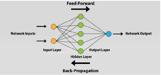
ANN is based on an assemblage of connected elements or nodes called neurons. Neurons act as channels that take an input, process it, and then pass it to other neurons for further processing. This transaction or the process of transferring data between neurons is handled in layers. Layers consist of at least three layers, input layer, one or more of hidden layers and output layer. Each layer holds a set of neurons that takes input and process data and finally pass the output to other neurons in the next layer. This process is repetitive until the output layer has been reached, so
eventually, the result can be presented. ANN architecture is shown in the following figure as is also known as feed-forward, which values pass in one direction.
Figure 3. ANN architecture
The data that is being held in each neuron is called activation. Activation value ranges from 0 to 1. As shown in figure 3, each neuron is linked to all neurons in the previous layer. Together, all activations from the first layer will decide if the activation will be triggered or not, which is done by taking all activations from the first layer and compute their weighted sum [18].
𝑤1𝑎1+ 𝑤2𝑎2+ 𝑤3𝑎3+ ⋯ + 𝑤𝑛𝑎𝑛 (5) However, the output could be any number when it should be only between 0 and 1. Thus, specifying the range of the output value to be within the accepted range. It can be done by using the Sigmoid function that will put the output to be ranging from 0 to 1. Then the bias is added for inactivity to the equation so it can limit the activation to when it is meaningfully active.
𝜎(𝑤1𝑎1+ 𝑤2𝑎2+ 𝑤3𝑎3+ ⋯ + 𝑤𝑛𝑎𝑛 − 𝑏) (6) Where 𝑎 is activation, 𝑤 presents the weight, 𝑏 is the bias and 𝜎 is the sigmoid function. Nevertheless, after getting the final activation, its predicted value needs to be compared with the actual value. The difference between these values is considered as an error, and it is calculated with the cost function. The cost function helps to detect the error percentage in the model, which needs to be reduced. Applying back-propagation on the model reduces the error percentage by running the procedures backwards to check on how the weight and bias are affecting the cost function.
Back-propagation is simply the process of reversing the whole activations transference among neurons. The method calculates the gradient of the cost function concerning the weight. It is performed in the training stage of the feed-forward for supervised learning [19].
3. Method
This study has been organised through theoretical research and practical implementation of regression algorithms. The theoretical part relies on peer-reviewed articles to answer the research questions, which is going to be detailed in section 4. The practical part will be performed according to the design described below and detailed furthermore in section 5.
3.1. Literature Study
Most of the literature study is based on articles with full text online, open access articles and peer-reviewed publications from Kristianstad University database search engine Summon, and the search websites; the Research Gate publications and the Towards Data Science collection instead of textbooks and chapters of books. The literature study endeavours to construct a robust basis on regression techniques, regularisation, and artificial neural network in machine learning and on how it can precisely be applied to house prices prediction.
The literature study gives an overview of the articles that are related to this study, the feature engineering methods that have been used in this study. As well as evaluation metrics that are used to measure the performance of the algorithms. In addition, the factors that have been used in the local dataset.
3.2. Experiment
The experiment is done to pre-process the data and evaluate the prediction accuracy of the models. The experiment has multiple stages that are required to get the prediction results. These stages can be defined as:
- Pre-processing: both datasets will be checked and pre-processed using the methods from section 4.2. These methods have various ways of handling data. Thus, the pre-processing is done on multiple iterations where each time the accuracy will be evaluated with the used combination.
- Data splitting: dividing the dataset into two parts is essential to train the model with one and use the other in the evaluation. The dataset will be split 75% for training and 25% for testing.
- Evaluation: the accuracy of both datasets will be evaluated by measuring the R2 and RMSE rate when training the model alongside an evaluation of the actual prices on the test dataset with the prices that are being predicted by the model.
- Performance: alongside the evaluation metrics, the required time to train the model will be measured to show the algorithm vary in terms of time.
- Correlation: correlation between the available features and house price will be evaluated using the Pearson Coefficient Correlation to identify whether the features have a negative, positive or zero correlation with the house price.
3.2.1. Evaluation Metrics
The prediction accuracy will be evaluated by measuring the R-Squared (R2), and Root Mean Square Error (RSME) of the model used in training. R2 will show if the model is overfitted, whereas RSME shows the error percentage between the actual and predicted data, which in this case, the house prices.
3.2.2. Computer Specifications
The needed time to train the model depends on the capability of the used system during the experiment. Some libraries use GPU resources over the CPU to take a shorter time to train a model.
Table 1. Computer Specifications
Operating System Windows 10
Processor Core i7 7700k
RAM 16 GB
Graphics card 1080 TI OC
3.2.3. Algorithms' Properties/Design
The algorithms used in this study have different properties that will be used during the implementation. The experiment is done with the IDE Spyder using Python as a programming language. However, in all algorithms, the data is split into four variables, namely, X_train, X_test, y_train, and y_test, by using train_test_split class from the library sklearn.model_selection. In addition, in all algorithms, the train_test_split class takes as parameters the independent variables, which is the data, the dependent variable, which is the SalePrice, test_size = 0.25, and random_state = 0. The properties and design of each algorithm are as below:
- Artificial neural network:
ANN is implemented with the feed-forward architecture as in figure 3 using Keras framework that does not include the back-propagation implementation. The model consists of an input layer, three hidden layers and the output layer. These layers contain a number of neurons which varies in both datasets. in the public dataset, the layers have 70, 60, 50, 25, 1 neurons, respectively. On the other hand, the layers in the local dataset have 64, 64, 64, 64, 1 neurons, respectively. The activation function used in this design is RELU for both datasets and the optimiser used is ADAM. The selection of the number of neurons, number of layers, activation function and the optimiser has been selected after running multiple tests to determine the one with the best performance. - Multiple linear:
Multiple linear is implemented using the LinearRegression from the library sklearn.linear_model. This library takes only the independent variables and dependent variable as parameters.
- Random Forest:
Random forest is implemented using the sklearn.ensemble.RandomForestRegressor library. This library takes several parameters to set up the model properties. The model consists of 1200 tree where the max depth of the tree is set to 60.
- Lasso Regression:
Lasso regression is implemented by using LassoCV class, which is from sklearn.linear library. The model LassoCV has several parameters that are set to prepare the model for the training. These parameters consist of the value of alphas = [1, 0.1, 0.01, 0.001, 0.0005], selection = random, and max_iter = 15000.
- Ridge Regression:
Ridge regression is implemented by using both Ridge and GridSearchCV classes. GridSearchCV class is from sklearn.model_selection library, which takes as parameters Ridge class, ridge parameter. This class performs grid search, and hyperparameter tuning to find the optimal parameter. Before fitting the Ridge model with the dataset, the class takes the best estimator method from GridSearchCV class and apply it for the model.
4. Literature Study
4.1. Related Work
There is a vast amount of work that is focused on training models to detect patterns in datasets to predict what the future output could be. However, there are researches where the authors use different machine learning algorithms with a combination of pre-processing data methods. A research was conducted in 2017 by Lu, Li and Yang [20]. They examined the creative feature engineering and proposed a hybrid Lasso and Gradient boosting regression model that promises better prediction. They used Lasso in feature selection. They used the same dataset as the one used in this study. They did many iterations of feature engineering to find the optimal number of features that will improve the prediction performance. The more features they added, the better the score evaluation they receive from the website Kaggle. Hence, they added 400 features on top of the 79 given features. Furthermore, they used Lasso for feature selection to remove the unused features and found that 230 features provide the best score by running a test on Ridge, Lasso and Gradient boosting.
In 2016, Jose Manuel Pereira, Mario Basto and Amelia Ferreira da Silva performed a study to examine three methods [21]. Lasso, Ridge and Stepwise Regression implemented in SPSS to develop an empirical model for predicting corporate bankruptcy. They defined two types of errors. The first error is the percentage of failed enterprises predicted well by the model. The second error is the percentage of good enterprises predicted failed by the model. The results of this study showed that the lasso and ridge algorithms tend to favour the category of the dependent variable that appears with heavier weight in the training set when they are compared to the stepwise algorithm implemented in SPSS.
A study was accomplished in 2017 by Suna Akkol, Ash Akilli, Ibrahim Cemal [22], where they did a comparison of Artificial neural network and multiple linear regression for prediction. In their study, the impact of different morphological measures on live weight has been modelled by artificial neural networks and multiple linear regression analyses. They used three different back-propagation techniques for ANN, namely Levenberg-Marquardt, Bayesian regularisation, and Scaled conjugate. They showed that ANN is more successful than multiple linear regression in the prediction they performed.
A research was done in 2010 by Reza Gharoie Ahangar, Mahmood Yahyazadehfar and Hassan Pournaghshband [23]. The authors estimated the stock price of activated companies in Tehran
(Iran) stock exchange by using Linear Regression and Artificial Neural Network algorithms. The authors considered ten macroeconomic variables and 30 financial variables. Then, they obtained seven final variables, including three macroeconomic variables and four financial variables, to estimate the stock price using Independent Components Analysis (ICA). They showed that the value of estimation error square mean, the absolute mean of error percentage and R2coefficient will be decreased significantly after training the model with ANN.
A study was conducted in 2015 by Nils Landberg [24]. Nils analysed the price development on the Swedish housing market and the influences of qualitative variables on Swedish house prices. Landberg has studied the impact of square meter price, population, new houses, new companies, foreign background, foreign-born, unemployment rate, the number of breaks-in, the total number of crimes, the number of available jobs ranking. According to Nils, unemployment rate, number of crimes, interest rate, and new houses have a negative effect on house prices. Landberg showed that the real estate market is not easy to be analysed compared with goods market because many alternative costs are affecting the increase in house prices. The study shows that the increase in population and qualitative variables have a positive effect on house prices. The interest rate, the average income level, GDP, and the fokus 8 In contrast, the rise in interest rates has a significant negative influence on house prices. Besides, it showed unemployment rate effects negatively on house prices, but the sale price and unemployment rate are not directly correlated with each other.
Research Question 1:
4.2. Feature Engineering
Feature Engineering is the technique of improving the performance on a dataset by transforming its feature space, and it is the practice of constructing suitable features from given features of the dataset, which leads to improving the performance of the prediction model [25]. However, several techniques should be implemented for better performance and a prediction result [26].
4.2.1. Imputation
Missing value imputation is one of the biggest challenges encountered by the data scientist. In addition, most machine learning algorithms are not powerful enough to handle missing data. Missing data can lead to ambiguity, misleading conclusions, and results [27]. There are two types of missing values [28]; the first type is called missing completely at random (MCAR). MCAR can be expressed as:
𝑃(𝑅|𝑋, 𝑍, 𝜇) = 𝑃(𝑅|𝜇) (7)
Where 𝑅 is the response indicator variables, 𝑋 are independent of data variables, and 𝑍 is latent. The second type is called missing at random (MAR), which can be expressed as:
𝑃(𝑅 = 𝑟|𝑋 = 𝑥, 𝑍 = 𝑧, 𝜇) = 𝑃(𝑅 = 𝑟|𝑋0 = 𝑥0) (8)
𝑓𝑜𝑟 𝑎𝑙𝑙 𝑥𝜇, 𝑧 𝑎𝑛𝑑 𝜇 (9)
There are two methods of handling missing data, namely ignoring missing data and imputation of missing data. Ignoring missing data is a simple technique which deletes the cases that contain missing data. The disadvantages of this method are that it reduces the size of the dataset, and it uses a different sample size for different variables. Imputation of missing data is a technique that replaces missing data with some reasonable data values [27]. However, the imputation of missing data method has two types, single imputation, and multiple imputations. Single imputation contains several approaches, such as mean imputation and regression imputation. Mean imputation is the most common approach of missing data replacement [27]. It replaces the missing data with sample mean or median. However, it has a disadvantage which is if missing data are enormous in number, then all those data are replaced with the same imputation mean, which leads to change in the shape of the distribution. Regression imputation is a technique based on the assumption of the linear relationship between the attributes. The advantage of regression imputation over mean imputation is that it was able to preserve the distribution shape [27].
4.2.2. Outliers
Outliers are noisy data that they do have abnormal behaviour comparing with the rest of the data in the same dataset. Outliers can influence the prediction model and performance due to its oddity. There are three types of outliers, which are point, contextual, and collective outliers [29]. Point outlier is an individual data instance that can be considered as odd with respect to
the rest of the data. The contextual outlier is an instance of data that can be regarded as odd in a specific context but not otherwise. An example of contextual is the longitude of a location. A collective outlier is a collection of related data instances that can be considered as abnormal with respect to the entire dataset. In supervised, the detection of outliers can be accomplished visually, where a predictive model is built for normal against outliers' classes. Dean De has investigated the public dataset and he suggests to remove certain outliers from the public data when he said "I would recommend removing any houses with more than 4000 square feet from the data set" [30]. Another example of detecting outliers is by using Isolation forest, which has two stages, training, and testing. The training is to create the isolation trees and then to record the anomaly score of each entry in the testing stage. This method has shown a promising result, according to [31].
4.2.3. Binning
Binning is a technique purposed to reduce the impact of statistical noise, to prevent overfitting, reduce overall complexity and make the model more robust. An interval with all observed values is split into smaller sub-intervals, bins, or groups [32]. Also, binning can be considered as a form discretisation, which is a technique to cut a continuous value range into a finite number of sub-ranges, where a categorical value is associated with each of them. Although there are several binning methods, this report is limited to equal-width, equal-size, and multi-interval discretisation binning. Equal-width binning is an approach where the whole range of predictor values is divided into a pre-specified number of equal-width intervals. Equal-size binning is an approach where the variety of predictor values is split into intervals in a way that bins contain an equal number of observations. However, the width of bins depends on the density of observations. Multi-interval discretisation binning is based on entropy minimisation heuristic search for recursively splitting of continuous range into sub-intervals [32]. The entropy function is defined as:
𝐸𝑛𝑡(𝑆) = − ∑ 𝑃(𝐶𝑖, 𝑆) log(𝑃(𝐶𝑖, 𝑆)) 𝑘
𝑖=1
(10)
Where 𝐶𝑖 are predictor classes in input dataset 𝑆, where maximising information entropy of the partition induced by 𝑇: 𝑆1 ∈ 𝑆, 𝑆2 = 𝑆 − 𝑆1 is given by:
𝐸(𝑇, 𝑆) =|𝑆1|
|𝑆| 𝐸𝑛𝑡(𝑆1) + |𝑆2|
Once cut point 𝑇 is found for compete interval of 𝑆, the process is repeated for sub-intervals recursively until there is no substantial improvement in entropy.
4.2.4. Log Transformation
A log transformation is a method that is used to handle skewed data. It is used to make data conform to normality, it reduces the impact of the outliers, due to the normalisation of magnitude and to reduce the variability of data [33].
4.2.5. One-hot Encoding
One-hot encoding is a technique that is used to convert categorical features to a suitable format to be used as an input in Machine Learning algorithms [34]. It transforms a single variable with 𝑛 observations and 𝑑 distinct values to 𝑑 binary variables, where each observation indicating the presence as 1 or absence as 0 [35]. In one-hot encoding, the categories are represented as independent concepts.
4.2.6. Feature Selection
Feature Selection is an important technique that is used to handle high-dimensional input data and overfitting caused by a curse of dimensionality by selecting a relevant feature subset based on mutual information criterion [36]. Moreover, feature selection has many advantages, such as improve the prediction performance by reducing dimensionality in the dataset. It speeds up the learning process and leads to a better understanding of the considered problem. However, there are many useful methods for feature selection, such as Mutual Information (MI) and Conditional Mutual Information (CMI) [37]. Mutual information is used for quantifying the mutual dependence of random variables, and it can be considered as the amount of information shared by two variables. MI is given as:
𝐼(𝑋; 𝑌) = ∑ ∑ 𝑝(𝑥𝑦)𝑙𝑜𝑔 𝑝(𝑥𝑦)
𝑝(𝑥)𝑝(𝑦) 𝑦∈𝑌
𝑥∈𝑋
(12)
Where 𝑥 ∈ 𝑋 and 𝑦 ∈ 𝑌 are the possible value assignments of 𝑋 and 𝑌, and 𝑙𝑜𝑔 is used base 2. Conditional Mutual Information measures the limited dependence between two random variables given the third [37].
𝐼(𝑋; 𝑌|𝑍) = ∑ 𝑝(𝑧) 𝑧∈𝑍 ∑ ∑ 𝑝(𝑥𝑦|𝑧)𝑙𝑜𝑔 𝑝(𝑥𝑦|𝑧) 𝑝(𝑥|𝑧)𝑝(𝑦|𝑧) 𝑦∈𝑌 𝑥∈𝑋 (13)
If 𝐼(𝑋; 𝑌|𝑍) = 0, 𝑋 and 𝑌 are conditionally independent given 𝑍.
4.3. Evaluation Metrics
Several evaluation metrics measure the performance of machine learning algorithms such as Mean Squared Error (MSE), Root Mean Squared Error (RMSE), R-Squared, and Mean Absolute Error (MAE). However, in this study, the performance of the algorithms is measured by using RMSE and R-Squared.
Root Mean Square Error (RMSE) is used as an evaluation metric in machine learning to measure the performance of the model. However, RMSE is similar to the Mean Square Error (MAE). Where all errors in MAE have the same weight, but RMSE penalises the variance, which means it gives more weight to the errors that have large absolute values than that have small absolute values. Therefore, when RMSE and MAE are calculated, RMSE is always bigger than MAE. RMSE is more sensitive to the errors than MAE; therefore, using RMSE for measuring the performance is better than MAE [38]. RMSE can be calculated as the square root of the sum of squared errors∑ (𝑦𝑛 𝑖 − 𝑦̂)𝑖 2
𝑖 over the sample size 𝑛. RMSE can be presented as: 𝑅𝑀𝑆𝐸 = √∑ (𝑦𝑖 − 𝑦̂)𝑖 2 𝑛 𝑖=1 𝑛 (14)
It can be observed from the equation when the sum of squared errors is closer to zero, RMSE is closer to zero. Therefore, when RMSE is zero, it means there are no errors between the actual value 𝑦 and the predicted value 𝑦 ̂.
R-Squared or as known as coefficient determination is a statistical measurement that is used in machine learning to measure how close the data are to the fitted regression line. R-Squared takes the value between 0 and 1. Where 1 indicates the prefect score and 0 is imperfect. In addition, R-Squared is calculated by measuring the deviations of the observations from their predicted values over the measurement of the deviations of the observations from their mean. R-Squared can be presented as:
𝑅2 = 1 − ∑ (𝑦𝑖 − 𝑦̂)𝑖 2 𝑖
∑ (𝑦𝑖 𝑖 − 𝑦̅)2
Where 𝑦 is the model, 𝑦̅ is the mean of the model, and 𝑦 ̂ is the prediction model of 𝑦. It can be observed when the sum of squared errors ∑ (𝑦𝑖− 𝑦̂)𝑖 2
𝑖 Is closer to zero and R-Squared is closer to one [39].
4.4. Research Question 1 Results
Several studies have been performed on or between multiple machine learning algorithms in order to predict and compare the prediction accuracy of the models. These studies indicate that an algorithm has performed better in their prediction results such as Artificial Neural network (ANN), which gives better accuracy results when it is compared with multiple linear regression [22]. However, the percentage of root square (R2) decreases after training the ANN model which means that ANN is prone to overfitting [23] that it might have an impact on the prediction accuracy in the final evaluation.
Data pre-processing is an essential part of preparing the data to be used by the training model. It does improve the prediction accuracy according to [26]. However, several problems might arise while dealing with the data. For instance, managing the missing values is a difficult task that can be solved in anyways. Hence, it requires a set of iterations before settling on a final solution. Moreover, outliers are noisy values within the dataset. Its existence affects the training model and preferably to be removed. It can be removed either by following suggesting of [30] which is to be tested alongside Isolation Forest. However, these studies evaluate the accuracy of the prediction with evaluation metrics and not the time need to train a model with the algorithm. In this study, the performance in terms of time is taken into consideration.
Research Question 2
4.5. Factors
There are many factors that influence the house prices. Some of these factors influence positively, whereas others have a negative impact on house prices [24]. The factors addressed in this section are Crime, interest, unemployment, inflation rate.
4.5.1. Crime Rate
Crime rate is the number of crimes that are perpetrated in a period of time. There are different types of crimes, such as burglary, vandalism, theft, assault, and robbery. However, the high level of crime rate leads people to move out to another place where the level of crime rate is low. The number of people who are willing to buy houses in neighbourhoods that have a high
level of crime rate will decrease, and that leads to a decrease in house prices. Therefore, the house prices will decrease in neighbourhoods that have a high level of the crime rate [40].
4.5.2. Interest Rate
Interest rate is the ratio of a loan that is charged as an interest to the borrower. However, the Swedish Central Bank [41] has divided the interest rates into three categories, which they are Repo, Lending, and deposit rates. Repo rate is the rate that is determined by the central bank of a country when it comes to lending money to other banks in case of any shortfall of funds in other banks [42]. The lending rate is the amount of money that banks charge others for lending its money. The deposit rate is the amount that banks pay for deposit holders in order to lure customers into putting their money in the bank. However, the interest rate plays a major role in clarifying the fluctuations in house prices in Sweden [19]. In addition, the low-interest rate has participated in increasing house prices [43].
4.5.3. Unemployment Rate
The unemployment rate is the ratio of people that do not have a job or looking for a job. However, the high level of unemployment is harmful to society because it reduces the GDP, it causes a loss of people's wealth, and it leads to lower taxes and higher expenses, which affect the government [44]. In addition, the unemployment rate affects as well as the house prices. High level of unemployment indicates that there are many people who do not have jobs and cannot afford to buy houses, which leads to decrease the house prices in order to lure people into buying houses [45].
4.5.4. Inflation Rate
The inflation rate is the percentage of increasing or decreasing in prices of goods and services. However, the high level of inflation reduces the purchasing power of the currency. Therefore, increasing of inflation rate leads to increase house prices [24].
4.6. Correlation
Correlation analysis defines the strength of a relationship between two variables, which can be between two independent variables or one independent and one dependent variable. The strength of the relationship can be distinguished based on direction and dispersion strength as in figure 4.
Figure 4. Correlation strength of the value of R
However, the correlation can be presented as a numerical value, which is called the correlation coefficient [46]. The value of the correlation coefficient ranges between 1 and -1. However, the correlation coefficient with a positive sign indicates that the two variables are positively correlated, which means when a variable increases the other increases as well. The correlation coefficient with a negative sign indicates that the two variables are negatively correlated, which means when a variable increases the other decreases. In addition, when the value of the correlation coefficient is closer to either positive one or negative one means the strength of the relationship between the two variables is strong. However, when the value of the correlation coefficient is closer to zero means the strength of the relationship between the two variable is weak, where the zero value indicates to non-relationship between variables.
4.7. Research Question 2 Results
The theoretical results show that many factors have an impact on house prices, such as the unemployment rate, the total number of crimes, interest rate, GDP, and population. However, it is difficult to analyse the real estate market compared with goods market, because the real estate market has more variables to examine [24]. However, the theoretical study shows that the increase in population, inflation and qualitative variables have a positive effect on house prices [24]. As well as the theoretical study shows that there are some factors that affect house prices negatively. The crime rate has a significant negative impact on house prices, according to [40]. Interest rate plays a major role in the fluctuation of house prices [47], and it has a negative correlation with house prices, which means low-interest-rate leads to increase the house price [43], Unemployment rate affects the GDP of the country, and it affects the government of the country leading to low taxes and high expenses [44]. Unemployment rate
affects negatively house prices, which means high level of unemployment rate leads to decrease house prices as reported by [45].
5. Experiment
5.1. Data Used
There are two datasets used in this study; they are named public and local datasets. The public dataset is taken from a website called Kaggle. It consists of records ranging from 2006 to 2010 in Ames, Iowa, United States. Each record contains 80 features describing an individual house, such as SalePrice, YearBuilt, YrSold, etc. The feature SalePrice is the variable to be predicted, and it will be taken out. Thus, 79 features are left, 37 of them are numeric, and the rest are categorical. A list with all features is available at [Appendix A].
The local dataset is brought from Svensk Mäklarstatistik [3]. It contains 9136 entries of sold houses " villas" ranging from 2009 to 2019 in Malmö, Sweden. However, it has 13 features, 6 numerical and 7 categorical features. These features are available at [Appendix B].
The local data has few features, and some of them got removed later in the process. Some features are added to the list to check their correlation with the house prices in the dataset, such as unemployment rate from ekonomifakta [48], Crime rate from brå [49], inflation rate from SCB [50], the repo rate, lending rate and deposit rate from SCB [41].
The source code for the experiment can be accessed from [Appendix C].
5.2. Public Data
This data came divided from the competition. There are train and test datasets. Thus, the experiment began by preparing the data to perform an initial prediction. Starting by checking if there are any missing values. The graph below shows the percentage of missing values in each feature.
Figure 5. Missing values in train data; public dataset
PoolQC, MscFeature and Alley have more than 80% of missing data. Therefore, these values can be resolved by replacing the missing data by calculating the mean value for numerical values and by replacing it with NONE for categorical values. However, some of these features are categorical, and the model accepts only numerical values. Thus, transforming them by using label encode and one-hot encode are required which work to replace each instance in a feature with a number that would help to identify it, as shown in table 2 and table 3.
Table 2. after applying label encoding
Index LotConfig LotConfiq_labelEncoding SalePrice
0 Inside 2 208500
1 FR2 1 181500
2 Inside 2 223500
3 Corner 0 140000
Table 3. After applying one-hot encode
Index LotConfiq_Corner LotConfiq_FR2 LotConfiq_Inside SalePrice
0 0 0 1 208500
1 0 1 0 181500
2 0 0 1 223500
3 1 0 0 140000
4 0 1 0 250000
Now the data is almost ready for the first prediction test; it needs to be separated from the house prices to get two data drafts called Train and SalePrice. Both are used to train the model, which gives the results below.
Table 4. First prediction results
Multiple Linear Lasso Ridge Random Forest
ANN
R2 0.6971 0.6953 0.6966 0.8555 0.6593
RMSE 44717.9238 44853.7815 44754.3819 30880.0679 28194.8593
R2 shows the measurement of data fitted in the training model, where the score is closer to 1 the data is more fitted in the model. RMSE shows the difference between the actual and predicted values. RMSE should be closer to 0 for the best score. The first prediction results show that the model is well fitted by looking at R2 scores and bad scores in RMSE.
Figure 6. Positive distribution of SalePrice
Figure 7. Skewness in SalePrice
Figure 8. Distribution after log transformation Figure 9. Skewness after log transformation
In figure 6, the plotting shows that the SalePrice distribution has positive skewness. This skewness effects the RMSE negatively. It can also be observed by plotting the values after they have been ordered as in figure 7. It can be resolved using Log transformation to be equally distributed, as shown in figure 8 and 9.
Table 5. Results after log-transformation
Multiple Linear Lasso Ridge Random Forest ANN
R2 0.7422 0.7390 0.7443 0.8830 0.7541
RMSE 0.0850 0.0855 0.0846 0.0572 0.0624
The result enhances when applying log transformation. As shown in table 5, R2 and RMSE scores have been improved from the first test.
Furthermore, another method of improving the data is to remove outliers. This method has been tested over two strategies. The first one is by finding the outliers manually from the graphs of plotting each feature over the SalePrice to check for anomaly values as suggested by [30]. The second is by using a library that helps detect anomaly rows called IsolationForest. Both
strategies have been tested. However, IsolationForest gave better outliers detection and prediction output. It caught 104 rows with outliers and 1356 without, out of 1460 rows in total.
Table 6. Prediction results after removing outliers
Multiple Linear Lasso Ridge Random Forest ANN
R2 0.8926 0.8909 0.8939 0.8825 0.4411
RMSE 0.0505 0.0509 0.0502 0.0528 0.0882
The results have improved further after removing outliers. Ridge scores the best result here by having the highest R2 and lowest RMSE scores. However, R2 has significantly dropped for the ANN model. Hence, we have performed a test to evaluate this drop. The test as in described and discussed in [Appendix E] that the drop could be occurred due to some of the outliers have a relation with other nodes in the dataset that have impacted the R2 negatively.
Multiple features seem to be related to each other and can be combined into one. For instance, the house living area is divided into three columns, 1stFlrSF, 2ndFlrSF, TotalBsmtSF. Also, some features have a lot of missing value due to its availability. Therefore, they have been replaced with Boolean to indicate their availability, such as the pool area. The new features and their sub-feature(s) are in the table below.
Table 7. Added features.
New feature List of sub-features
TotalSF GrLivArea, LotArea, TotalBsmtSF
Total_Bathrooms FullBath, HalfBath, BsmtFullBath, BsmtHalfBath Total_porch_sf OpenPorchSF, 3SsnPorch, EnclosedPorch, ScreenPorch,
WoodDeckSF
haspool PoolArea (Set to available of poolArea is not empty) has2ndfloor 2ndFlrSF (Set to available of 2ndFlrSF is not empty) hasgarage GarageArea (Set to available of GarageArea is not empty) hasbsmt TotalBsmtSF (Set to available of TotalBsmtSF is not empty) hasfireplace Fireplaces (Set to available of Fireplaces is not empty)
Binning the features improved the ANN result. However, it slightly affected the other algorithms as in the table below.
Table 8. Prediction results after creating new features
Multiple Linear Lasso Ridge Random Forest ANN
R2 0.8888 0.8912 0.8893 0.8836 0.8223
RMSE 0.0535 0.0529 0.0533 0.0547 0.0455
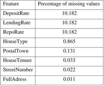
5.3. Local Data
The data will be pre-processed as the public data in section 5.2. The percentage of missing values in the data will be checked if available. List of the features with the rate of missing values of each are as presented in the table below.
Table 9. Percentage of missing values in local data
Feature Percentage of missing values
DepositRate 10.182 LendingRate 10.182 RepoRate 10.182 HouseType 0.865 PostalTown 0.131 HouseTenure 0.033 StreetNumber 0.022 FullAdress 0.011
The missing values will be resolved as in the public data, followed by applying label and one-hot encoding to make the data ready for the first test. Moreover, some features are dropped from the data because they are having the same values or redundant data that is already presented by other features. For instance, ContractDate since year and month are available, MunicipalityCode since it is shared with all entries and HouseCategory since all houses belong to the same category.
Table 10. Prediction results
Multiple Linear Lasso Ridge Random Forest ANN
R2 0.1818 0.1818 0.1819 0.3273 0.1782
RMSE 1613833.55 1613810.741 1613801.03 1463346.0745 1097759.5
Table 10 shows the R2 and RMSE rates after the first test. The results are as bad as the first prediction test on the public data. However, R2 scores are low, which means that the independent variables are not explaining much in the variation of the sale price, which is why the RMSE scores are high. In addition, ANN gave a negative R2 score in the first test, as shown in [Appendix D], where it should be within the range of 0 and 1. The design of ANN has been modified to use the same optimiser, ADAM, as used in the public data instead of the optimiser RMSPROP, which enhanced the results of ANN.
Another method is to apply log-transformation and remove outliers. IsolationForest has detected 3913 outliers leaving 5221 rows for training.
Table 11. Prediction results after pre-processing
Multiple Linear Lasso Ridge Random Forest ANN
R2 0.1874 0.1836 0.1872 0.3328 0.2591
RMSE 0.1371 0.1375 0.1372 0.1243 0.0993
RMSE score has improved from the last test, whereas R2 score has slightly improved; however, it is still low.
5.4. Correlation
The correlation gives an overview of the association strength between available features and the house price. The correlation is being calculated using the Pearson Coefficient Correlation method. In the public dataset, features have an impact on the sale price. Figure 10 shows the correlation with a positive sign in the public data.
Figure 10. Positive correlation in public data
On the other hand, figure 11 shows the features that have a correlation with a negative sign with house price.
Since there are not many features in the local data, figure 12 shows the correlation for all features in the local data.
Figure 12. Correlation in local data
5.5. Experiment Results
Many machine learning algorithms are used to predict. However, previous researches have shown a comparison between them alongside Artificial neural network in different datasets. Therefore, using these algorithms is beneficial so that the result can be as near to the claimed results. However, the prediction accuracy of these algorithms depends heavily on the given data when training the model. If the data is in bad shape, the model will be overfitted and inefficient, which means that data pre-processing is an important part of this experiment and will affect the final results. Thus, multiple combinations of pre-processing methods need to be tested before getting the data ready to be used in training.
5.5.1. Prediction Accuracy
Pre-processing methods played a significant role to provide the final prediction accuracy, as shown in the experiment sequence in both public and local data, as indicated by [26]. Resolving
outlier, as suggested by [30] gave a worse outcome than Isolation Forest [20] where it has improved the prediction accuracy.
The performance of trained models has been measured by evaluating the RMSE and R2 metrics, where RMSE needs to be closer to 0 and R2 closer to 1. The accuracy has been evaluated by plotting the actual prices on the predicted values, as shown below.
Figure 13. Prediction accuracy for public data
Figure 13 shows the final prediction accuracy after applying all used pre-processing methods on public data. The accuracy measures the actual data over the predicted data by the model. Thus, the closer to each other, the better prediction accuracy it is. From the graph, however, it is evident that ANN differs from the other algorithms by having a worse prediction despite that it has the best RMSE score which proves that R2 score decreases when training the ANN model [23]. Whereas regression algorithms show better accuracy, which is because, by looking at table 8, R2 and RMSE. Hence, Lasso has scored the highest R2 and lowest RMSE, indicating that its model is well fitted compared to other regression algorithms, which means that Lasso has the best prediction accuracy in public data.
However, ANN performed worse than multiple linear, giving the opposite result to what has been conducted by [22]. The difference between the results of [22] and this study is that ANN in this study was designed by using different design and where ANN in this study uses feed-forward architecture with a total of 5 layers, which are one input layer, 3 hidden layers, and one output layers. ANN in [22] is designed with 1 hidden layer and uses different back-propagation algorithms such as Levenberg-Marquart, Bayesian Regularization, Scaled Conjugate.
Figure 14. Prediction accuracy for local data
Figure 14 shows a worse accuracy compared with public data. The algorithms have achieved low RMSE and R2 scores, as shown in table 11. However, despite that the models are under fitted; the random forest has performed better than other algorithms due to it is being more fitted than other models.
ANN performed a slightly better prediction accuracy than Multiple linear here, which is as what is demonstrated by [22]. This comes down to that ANN has a higher R2 score which indicates that the training model is a bit more fitted to the data compared with Multiple linear in addition to them using a different dataset than the one used in this study.
Overall, the results show how the pre-processing methods on both public and local data make an enhancement to the model after each iteration as in section 5 as stated in [25]. Both datasets have a different number of features and rows, which could be a reason why the prediction accuracy differs. Also, the correlation strength in local data is weaker than the public data, which could also be another reason why the prediction is better in the public data.
5.5.2. Correlation
As shown in graphs 9 and 10, the correlation between SalePrice and other variable differs. The public dataset has a correlation, whether it has a positive or negative sign, which means that these variables provide a better prediction than others. However, Table 12 shows the features that have a correlation with a positive sign with the sale price.
Table 12. Correlation with a positive sign in public data
Feature Correlation Feature Correlation Feature Correlation
LotFrontage 0.36 BsmtFullBath 0.28 OverAllQual 0.79
LotArea 0.27 HalfBath 0.28 YearBuilt 0.52
3SsnPorch 0.045 BedroomAbvGr 0.17 YearRemodAdd 0.51
YearBuilt 0.53 Fireplaces 0.47 TotalBsmtSF 0.61
MoSold 0.05 GarageYrBlt 0.49 1stFlrSF 0.61
MasVnrArea 0.48 GarageArea 0.63 GrLivArea 0.71
BsmtFinSF1 0.39 WoodDeckSF 0.33 FullBath 0.56
BsmtUnfSF 0.22 OpenPorchSF 0.32 TotRmsAbvGrd 0.53
TotalBsmtSF 0.62 PoolArea 0.093 GarageCars 0.64
ScreenPorch 0.12 2ndFlrSF 0.32 GgaraggeArea 0.62
The negative correlation is an important factor as well since it affects the sale price negatively. Table 13 shows the features with a negative correlation with the sale price.
Table 13. Negative correlation in public data
Feature Correlation MSSubClass -0.08 OverallCond -0.08 LowQualFinSF -0.03 KitchenAbvGR -0.14 EnclosedPorch -0.13 YrSold -0.03 BsmtFinSF2 -0.01 BsmtHalfBath -0.02 MiscVal -0.02
However, the local dataset does not have many features. Therefore, all features that are correlated with sale price are combined in one table, as shown in table 14.
Table 14. Positive and negative Correlation in local data Feature Correlation Unemployment rate 0.12 Crime -0.27 Repo rate -0.27 Lending rate -0.26 Deposit rate -0.26 Inflation 0.14 Year 0.31 Month 0.04 Street number -0.10
The table shows that inflation, year, month, and unemployment rate have a weak positive correlation with the sale price. While crime, repo, lending, deposit rates, and a street number have a weak negative correlation with the sale price. The results show that the independent variables have an insignificant influence on the house prices in Malmö. Among these features, the year variable affects the sale price the most, which means that every year the house price increases. Besides, as the inflation rate increases, the house price goes up with it. The results show that when the number of crimes increases the house price decreases, and it is the same with repo, lending, and deposit rates when they increase the house price decrease.
5.5.3. Factors
The factors that have been discussed in section 4.5 and the features of houses in the local data are combined in order to study the correlation between them and the sale price, as in table 14. The correlation values show that the local dataset is weak since the correlation values of the features are close to zero, which indicates to non-relationship between the factors and the sale price.
However, table 14 shows that crime, repo, lending, deposit rates, and street number have a weak negative correlation with sale price (numbers are close to zero). It means when these factors increase the house price decrease. In addition, unemployment rate, inflation, year, and month have a weak positive correlation with the sale price (numbers are close to zero). It means when these factors increase the sale price increase.
The data of repo, lending, and deposit rates are added to the local dataset where they have entries from 2010 to 2019, and the local dataset contains records from 2009 to 2019. Therefore, mean imputing has applied to fill the missing values in the repo, lending, and deposit rates. The theoretical result shows that crime rate [40], interest rate [43], and unemployment rate [45] have a negative influence on house prices indicating that when these factors increase the house price decrease. The empirical results show that the crime rate, repo, lending, and deposit rates have a weak negative correlation with the sale price. Due to its weakness, it may indicate that when these factors increase the house price decrease. In addition, the theoretical result shows that inflation has a positive impact on house prices [24], indicating that when inflation increases the house prices increase. The empirical result shows that inflation and year have weak positive correlations, and it may indicate that when these factors increase the house prices increase. However, the theoretical result shows that the unemployment rate has a negative influence on house prices, whereas the empirical shows that the unemployment rate has a weak positive correlation to the sale price. This error can be justified due to the weakness of local dataset, which means when the dataset is weak, it may give wrong results.
6. Discussion
This study was conducted on two different datasets, public and local. The public data set has 80 features and 1460 rows, and the local dataset has 9136 rows and a total of 13 features and 19 after adding the features presented in this study. However, the final trained model gave promising results regards the house prices.
Training of the ANN has shown that it is slower than other algorithms as in [appendix F], especially when it comes to large-size data. ANN frameworks utilise the CPU to process the data. However, there are additional GPU drives that allow the framework to make use of the GPU resources instead of the CPU. It has helped to speed up the training process rapidly when using a significant number of neurons in ANN.
ANN got affected negatively after eliminating the outliers when training the model with the public data. The R2 score got worse, which could fall into several reasons, such as the implemented design of ANN and removing important nodes from the dataset, which were considered as an outlier by the IsolationForest library. However, this gap has been resolved after applying the binning method presented in this study.
Applying the same algorithm that has the same property on two different datasets gives different results as the empirical results of the local and public datasets have shown. Lasso regression has the best score overall in the public dataset, and Random Forest regression has the best score overall in the local dataset. Although, we applied the same properties for the algorithms in both public and local datasets.
Working with two different datasets prove that it is difficult to use the same pre-processing methods with multiple datasets. The results have shown differences in accuracy and performance between the two datasets. Although the local and public datasets are similar in concept, they have different and unequal features. In addition, if another design used in the implementation, it would result in different prediction accuracy.
Furthermore, the correlation strength varies between the public and local dataset. The correlation shows that the stronger the relationship, the better the accuracy, as shown from the prediction accuracy in both datasets. Thus, the local dataset requires more features that would support it to raise the correlation strength and have a chance to achieve an accurate prediction model.
Data processing and feature engineering are crucial in machine learning to build a prediction model. Furthermore, a model cannot be made without some data processing. For instance, as shown in the experiment, the model could not be trained before handling the missing values and converting the text in the dataset into numerical values. Another example is that the results have shown that the algorithms did not predict accurately before log transformation on the sale price. Hence, from the experiment, we saw that pre-processing the data does improve the prediction accuracy and matches the result of [26].
Outliers have been resolved over two ways. They have been handled as suggested by [30] and by using Isolation Forest. Isolation forest made a better outlier's detection which led to a noticeable improvement in the RMSE and R2 scores when looking at the ANN, for example. Although this study has shown that Lasso made the best prediction, one cannot guarantee that it will perform the same when used for other purposes than the ones that have been presented in this study. An example of this can be seen from comparing Lasso's output when used in both public and local datasets. The accuracy differs due to the datasets not having the same characteristics.
Getting an overview of the correlation helped to understand the difference between the two datasets. It showed the value of some variables and their effect on the prediction. A weak dataset may result in an inaccurate prediction or correlation between the features. Results show that the correlation in the local data is weak and almost considered as zero correlation since the values are close to zero.
Question 1 – Which machine learning algorithm performs better and has the most accurate result in house price prediction? And why?
The practical results show that Lasso is the most accurate algorithm among other algorithms, and it has the best performance after evaluating both RMSE and R2. Lasso achieved 0.052 and 0.13 RMSE scores on public and local data, respectively. Lasso scored 0.8912 and 0.1836 R2 scores on public and local data, respectively. Besides, Ridge and Lasso have achieved 0.0533 and 0.0529. However, Random Forest has performed better than Multiple linear, Ridge and Lasso in the local dataset due to the weakness of the local dataset and the overfitting.