Development of Microwave sensor and Android Application for monitoringlong bone defects

(1)

IT 16 090

Examensarbete 30 hp

November 2016

Development of Microwave sensor

and Android Application for monitoring

long bone defects

Asad Hameed Afridi

Institutionen för informationsteknologi

Department of Information Technology

(2)

(3)

Teknisk- naturvetenskaplig fakultet UTH-enheten Besöksadress: Ångströmlaboratoriet Lägerhyddsvägen 1 Hus 4, Plan 0 Postadress: Box 536 751 21 Uppsala Telefon: 018 – 471 30 03 Telefax: 018 – 471 30 00 Hemsida: http://www.teknat.uu.se/student

Abstract

Development of Microwave sensor and Android

Application for monitoring long bone defects

Asad Hameed Afridi

Fractures of the long bones are one of the most common injuries. Long bone are always at risk for fractures and require careful treatment to avoid the human disabilities. Microwave technology is using to development of biomedical sensors for detecting and monitoring bone defects. Microwave are electromagnetic (EM) radiation with frequencies between 300MHz and 300 GHz. The microwave technology is used in wireless networking and communication systems, wireless security systems, remote sensing and medical application.

The main purpose of this thesis is to investigate rectangular microstrip patch antenna for monitoring long bone defects. A narrow band microwave antenna will be

designed, then validate the antenna using measurement. Design an application for mobile, where physicians can easily see the patient’s measurement in a graph form, healing process and physicians can analyze the patient’s health condition.

Tryckt av: Reprocentralen ITC IT 16 090

Examinator: Arnold Neville Pears Ämnesgranskare: Robin Augustine Handledare: Sujith Raman

(4)

Acknowledgements

I would like to thank Dr.Robin Augustine who gives me the opportunity to work his group and support of my thesis project. I would also like to thank my supervisor Sujith Raman. A special thanks of my co-supervisor Syaiful Mohd Shah Redzwan guidance during my project.

A special feeling of gratitude goes to my loving parents, sister and brothers, whose prayers and words of encouragement helped me to reach this point. They are also providing me with unfailing support and continuous encouragement throughout my years of study and through the process of researching and writing this thesis. This accomplishment would not have been possible without them.

I would also like thank to Jasmin Laroche in Uppsala University, she encouraged me a lot throughout my research work and gives feedback in my report. Finally, special thanks to my friends who have always been supportive and loving.

(5)

Table of Contents i

List of Figures

Figure 1 Classification of bones on the basis of shape [3] ... 1

Figure 2 Types of long-bone Fractures [4] ... 3

Figure 3 The three phases of the healing process [15] ... 4

Figure 4 Current analyzing system for Fracture bones [23] ... 5

Figure 5 Wire Antennas [31] ... 10

Figure 6 Aperture Antenna [31] ... 10

Figure 7 MIcrostrip Antenna Configuration [31] ... 11

Figure 8 Representative shapes of microstrip patch elements [31] ... 12

Figure 9 MIcrostrip Line feed [31] ... 12

Figure 10 Android OS architecture [39] ... 14

Figure 11 Java source to DVM byte code process [37]... 15

Figure 12 All Parameters of microstrip Line ... 18

Figure 13 Microstrip Antenna with Coaxial Probe ... 20

Figure 14 Return Loss of Microstrip Antenna with Coaxial Probe ... 20

Figure 15 L=16.42mm, W=22.82 and Y0 from 5.45 mm to 7.45 mm... 21

Figure 16 W = 22.82 mm, Y0 = 5.45 mm and L is from 15.42 mm to 18.42 mm ... 21

Figure 17 L=18.42 mm Y0 = 5.45 and W is change from 20.82 mm to 24.32 mm... 22

Figure 18 Microstrip Antenna with Microstrip Line ... 23

Figure 19 Return Loss of Microstrip Antenna with Microstrip Line ... 23

Figure 20 W = 22.82mm, y0= 6.45mm gap = 0.3 and L is from 17.12mm to 17.52 mm ... 24

Figure 21 W = 22.82mm, L=17.22mm, gap 0.3mm and Y0 change from 5.45 to 6745mm ... 24

Figure 22 W = 22.82mm, y0= 6.45mm gap = 0.3 and L is from 17.22mm to 17.50mm ... 25

Figure 23 Y0= 6.45 mm gap = 0.3 mm, L =17.50mm (a) change Wf (b) change W ... 25

Figure 24 Proposed System Architecture [23], [53], [55] ... 29

Figure 25 Sensor on Long bone model ... 31

Figure 26 Return loss of coaxial probe sensor in Free Space and body model. (Antenna: - L=18.42 mm Y0 = 5.45 mm and W = 18.42mm) (Model: - skin thickness =1 mm, fat thickness= 3.5 mm, muscle thickness = 13 mm and bone thickness = 50 mm) ... 31

Figure 27 Return loss of coaxial probe sensor to change thickness of skin. (Antenna: - L=18.42 mm Y0 = 5.45 mm and W = 18.42mm) (Model: - skin thickness change from 1 mm to 3.6 mm, fat thickness= 3.5 mm, muscle thickness = 13 mm and bone thickness = 50 mm) ... 32

Figure 28 Return loss of microstrip line sensor in Free Space and body model. (Antenna: - L=17.52 mm Y0 = 6.25 mm, W = 22.82mm and g=0.3 mm) (Model: - skin thickness =1 mm, fat thickness= 3.5 mm, muscle thickness = 13 mm and bone thickness = 50 mm) ... 32

Figure 29 Return loss of microstrip line sensor to change thickness of skin. (Antenna: - L=17.52 mm Y0 = 6.25 mm, W = 22.82mm and g=0.3 mm) a) Model:- skin thickness change from 1 mm to 3.6 mm, fat thickness= 3.5 mm, muscle thickness = 13 mm and bone thickness = 50mm ... 33

Figure 30 Return loss of microstrip line sensor to change thickness of skin. (Antenna: - L=17.52 mm Y0 = 6.25 mm, W = 22.82mm and g=0.3 mm) Model: - skin thickness 3, fat thickness= 11 mm, a )muscle thickness change from 13 to 25 b) bone thickness change from 50 ... 33

Figure 31 SSR Sensor on Long bone model [62] ... 34

Figure 32 Simulation and Phantom Result [62] ... 35

(8)

List of Figures iv

Figure 34 Web service on localhost ... 37 Figure 35 Android Application for bone healing ... 38 Figure 36 Application some basic setting ... 39

(9)

List of Tables v

List of Tables

Table 1 Classification of bones on the basis of shape [5] 2 Table 2 Return Loss and power Reflected from Antenna [34] 8 Table 3 Android versions and API level [39]–[42] 13 Table 4 Microstrip Antenna parameters specifications 19 Table 5 Different microstrip size antenna with Coaxial Probe feed technique 22 Table 6: Different microstrip size antennas with microstrip line feed technique 26 Table 7 The Minimum and Maximum thickness of the Human organs 30

(10)

List of Abbreviation vi

List of Abbreviation

Abbreviation

CT Computed tomography

MRI Magnetic Resonance imaging

EM Electromagnetic

VNA Vector Network Analyzers

SRR Split Ring Resonator

GUI Graphical User Interface

CST Computer simulation Technology IDE Integrated Development Environment

XML EXtensible Markup Language

SQL structured Query Language

RF Radio Frequency

dB Decibels

VSWR Voltages Standing Wave Ratio

VLF Very Low Frequency

LF Low Frequency

HF High Frequency

VHF Very High Frequency

GPS Global Positioning System

OS Operating System

OHA Open Handset Alliance

ASL/Apache2 Apache Software License

DVM Dalvik Virtual Machine

JIT Just In Time

APIs Application programming interfaces

GPS Global Positioning System

PCB Printed Circuit Board

Mm Millimeter

PEC Perfect Electrical Conductor

SMA Sub Miniature version A

JSON Java Script Object Notation IIS Internet Information Services

(11)

1

1 Introduction

1.1 Introduction

The Skeletal system is the main part of the human body and it maintains the shape of a human body. The skeleton is made up of bones and teeth. The normal human skeleton has 206 bones. The skeleton is divided into two parts: the Axial and the Appendicular skeleton [1]–[3]. The Axial skeleton consists of the thoracic cage, the vertebral column and the skull bones , while the Appendicular skeleton consists of the bones of the upper and lower extremities along with their associated girdles [2].

The skeletal system serves mechanical functions in the human body [3], [4] (a) Support: The skeleton helps to support and maintain the shape of the body.

(b) Movement: The skeleton consists of many bones. These bones have flexible muscles and joints which helps in the movements and is grabs in an objects.

(c) Protection: The bones protect different organs for example the skull protects the brain, the vertebrae surrounds the spinal cord, and the rib cage protects the vital organs of the thorax. The bones can also be classified into four groups by their shape, as shown in Figure 1 and Table 1.

(12)

Chapter 1 Introduction 2

Table 1 Classification of bones on the basis of shape [5]

Bone

classification

Features Functions Examples Long Cylinder-like shape,

longer than it is wide

Leverage Femur, tibia, fibula, metatarsals, humerus, ulna, radius, metacarpals, phalanges

Short Cube-like shape, approximately equal in length, width, and thickness

Provide stability, support, while allowing for some motion

Carpals, tarsals

Flat Thin and curved Points of attachment for muscles; protectors of internal organs

Sternum, ribs, scapulae, cranial bones

Irregular Complex shape Protect internal organs Vertebrae, facial bones

1.2 Long Bones

Long bones are long, wide and hard and have a shaft and two ends, as shown in figure 1. The Appendicular skeleton consists of long bones except the patella, the wrist and the ankle bones. They include Femur (leg bone), Tibia (leg bone), Fibula (leg bone), Humerus (arm bone), Ulna (arm bone) and Radius (arm bone) etc.…

1.2.1 Fracture of long bones

Fracture of the long bones is one of the most common injuries. Long bones can be cracked or completely broken at any place and in any direction. Fracture can happen in a variety of ways, but there are three common reasons: Trauma fractures (Accidents), Osteoporosis (bone disease or tumor may weaken a bone) and stress or overuse [4]. Fracture can be divided into two main groups simple fracture (close fracture) and compound fracture (open facture).

a) Simple fracture: when the fracture affects the soft tissue but does not damages the skin. b) Compound fracture: when the bone breaks and damage the skin. Such fracture is more risky

than a simple fracture.

Long bones fracture are divided into different patterns [4], [6]–[8], as shown in Figure 2. a) Simple Transverse Fracture: - when the bone is broken perpendicularly of the long axis of

bone.

b) Oblique Fracture – when the bone is broken an angle of long axis of bone is called oblique fracture.

c) Spiral Fracture – It is similar to the Oblique fracture but in this fracture the bone is broken in rotation along with the long axis of the bone.

d) Longitudinal Fracture – The longitudinal fracture is similar to the long oblique fracture, but the bone cracks parallel to the long axis of the bone.

e) Comminuted Fracture – the bone is broken into small pieces, multiple fragments are present.

(13)

Figure 2 Types of long-bone Fractures [4]

1.3 Problem Motivation

Long bones are always at risk for fractures and require careful treatment to avoid human disabilities. These fractures may be caused by several like accidents, or bone diseases. Bone fractures are a big health issue in the world.

In the United States of America in the year 2000, 50 million injuries required treatment at the cost of $406 billion, incidence of long bone fracture is 11.5 per 100,000 persons, with 40% occurring in the lower limb[9] in the United Kingdom was estimated at £726 million[10].

“In the year 2000 there were an estimated 9.0 million osteoporotic fractures of which 1.6 million were at the hip, 1.7 million at the forearm and 1.4 million were clinical vertebral fractures. The greatest number of osteoporotic fractures occurred in Europe 34.8%” [11].

“Osteoporosis causes over 1.5 million fractures each year in the USA, over 300,000 hips, 700,000 vertebral and over 250,000 wrist fractures“ [12].

“According to Osteoporosis Australia Medical & Scientific Advisory Committee “There is 1 fracture every 3.6 minutes in Australia (2013). By 2022 there will be one fracture every 2.9 minutes [13]”.

Bone healing is a complex process, and this process is divided into different stages and at each stage the physician needs to diagnose the fractured bone [14], [15]. Physicians prefer X-Ray, which is the most common procedure to diagnose bone fractures at a low cost. In some cases the physicians can also use other methods for diagnosis such as Computed tomography (CT) scan, Magnetic Resonance imaging (MRI) to detect different types of abnormalities [16]. The healing process is dependent on the patient’s age, fracture type and fracture location in the body, therefore it is hard to mention the estimated time for healing bone. The stages of the healing process overlap with one another and have no definitive beginning or end points [15], as shown in Figure 3.

(14)

X-ray is ionizing radiation, which is used for medical imaging. X-ray provides lot of benefits, but there is some risk for cancer. Children are more sensitive than adults, so there is a higher chance for children to be affected by x-ray radiation [17]. According to Amy Berrington de González and Sarah Darby in “the UK about 0·6% of the cumulative risk of cancer to age 75

years could be attributable to diagnostic X-rays. This percentage is equivalent to about 700 cases of cancer per year. In 13 other developed countries, estimates of the attributable risk ranged from 0·6% to 1·8%, whereas in Japan, which had the highest estimated annual exposure frequency in the world, it was more than 3%” [18].

Figure 3 The three phases of the healing process [15]

In bone fracture, the first 6 weeks are important. For the physicians to make sure that bone is healing properly, the physician can monitor the bone healing process in x-ray. In some conditions x-ray do not give accurate report about healing process [19] and there is no technology for physicians to use to continuously monitor (real time) the healing process. In order to provide better methods for monitoring bone healing the researchers have been working on implementing microwave technology in medical diagnostic devices. Prof. Robin Augustine (associate professor in Microwave Technology at the Solid state Electronics Division Uppsala University and Microwaves in Medical Engineering Group www.mmguppsala.se) is doing research on the development of biomedical sensors for detecting and monitoring bone defects using microwaves that aim for faster patient rehabilitation outcomes [20], [21]. Microwaves are electromagnetic (EM) radiation with frequencies between 300MHz and 300 GHz. Microwave is the non-ionizing radiation which is less hazardous than ionizing radiation. The microwave technology is used in wireless networking and communication systems, wireless security systems, remote sensing and medical application [22].

1.4 Related work and current working system

Microwave technology at Solid State Electronic Division Uppsala University utilizes split Ring Resonator Antenna as a probe to analyze the osseointegration of skull implants which helps to diagnose the bone implant reunion in children suffering from intracranial pressure [21].

(15)

The SRR (Split Ring Resonator) Antenna is attached to a miniVNA (Vector Network Analysers). The system is connected with computer though USB cable or integrated through Bluetooth module. The measurement data is saved from user interface in different file formats however Prof. Robin Augustine’s group keep data in s1p file format, as shown in Figure 4. The steps involved in patient measurements

a) Free space measurement of SRR Antenna

b) SRR antenna is placed on the patient’s healthy bone area for reference c) SRR antenna is placed on the patient’s fracture bone in different area

Measurement results are kept in s1p format file and then used for future analyzing.

Figure 4 Current analyzing system for Fracture bones [23]

1.5 Aim and Scope of Work

The aim of this thesis is to investigate the rectangular microstrip patch antenna as a sensor which can analyze fractured bones and to program the mobile application for that sensor. The thesis is divided two different section, the first section is analyzes the rectangular microstrip patch antenna as sensor and the second developed the mobile application. In the current working system all data is saved in file format. There is no centralized database to store the patient’s data for analysis. The research group imports the measurement file into the VNA/J GUI application [23] to compare the patient’s measurements and check the healing process. The VNA/J GUI is the general purpose application for the miniVNA device.

1.6 Tool Kit

The following tools have been used for antenna design and development of a mobile application a) CST Studio

Currently Microwaves in Medical Engineering Group is using the CST studio for antenna design. The Electromagnetic Simulation Software CST studio is used in research of electromagnetic design. The CST studio consists of many modules. The CST microwave studio is the leading edge tool for fast and accurate 3D simulation of high frequency devices in time and frequency domain. This module is used for antenna design[24].

(16)

b) Android Studio

Android Studio is Android’s official IDE (integrated development environment) for creating android application. It is freely available. Applications are primarily written in java programming language and most of the android configuration files are based on XML (EXtensible Markup Language). The project is developed in the android system which is called AOSP (Android Source Project) and the project should be available on Google play [25], [26]. The mobile application is developed in Android Studio.

c) Matlab

Matlab is used to simplify and process antenna design equation. d) SQL server 2014

The SQL (structured Query Language) server includes several data management and analysis technologies. Users can easily design databases for any application and used for future analysis[27]. This tool is used to make a small database for the patient’s records and bones fracture measurements. Database is connected to web service and also to Window Application.

e) Visual studio 2015

Visual Studio is extensible IDE for professional teams, individual developers and academic research. It can be used to develop applications for Windows, web application and cloud serveries[28]. This IDE is used to develop a small window application to keep patient’s measurements in the SQL database, and IDE is used to develop web service.

(17)

7

2 Antenna theory

2.1 Antenna Theory

In the radio systems Antenna is an important device for communication in the free space. This device transmits electromagnetic waves in the free space or receives electromagnetic (RF, Radio frequency) waves from the free space. The transmitter and receiver are working at same frequency band of the radio system to which they are connected [29], [30].

The theoretical foundation of electromagnetic theory is based on Maxwell’s Equations. In 1886 the German physicist Heinrich Hertz was able to verify experimentally and validate Maxwell’s equation of the electromagnetic waves. Marconi who developed radio communication, is considered to be the father of radio [22], [30].

The fundamental electromagnetic equation are [22], [30]

∇. D = ρv (2.1) ∇. 𝐵 = 0 (2.2) ∆ × 𝐸 =𝜕𝐵 𝜕𝑡 (2.3) ∇ × 𝐻 = 𝜕𝐷 𝜕𝑡 + 𝐽 (2.4) ∇. 𝐽 = − 𝜕 𝜕𝑡 ρv (2.5)

First four are Maxwell’s equation and last one is continuity equation.

2.2 Properties of Antenna

2.2.1 Wave length

Antenna size is dependent on wave length. 𝜆 =𝑐

𝑓 (2.6)

𝜆 is the wavelength, c is the speed of light and f is the frequency. 𝜆 is inversely proportional to f. The higher frequency shorter the wavelength.

2.2.2 Input Impedance

The input impedance parameter is important to transfer energy efficiently. To transfer maximum power, the input impedance of the antenna should match with the source. If the impedance of antenna is mismatched the power will be reflected back to the source [30], [31]. The input impedance is composed of real and imaginary parts [30], [32]

𝑍_𝑖𝑛 = 𝑅_𝑖𝑛+ 𝑗𝑋_𝑖𝑛 (2.7)

Where 𝑍𝑖𝑛 is the Antenna impedance, 𝑅𝑖𝑛 is the input resistance and 𝑋𝑖𝑛 is input reactance

(18)

Chapter 2 Antenna and Android theory 8

2.2.3 Band Width

Band width can be defined as the range of frequencies where the antenna can operate correctly. For broadband antennas the band width is expressed in ratio and narrowband antennas band width is express in percentage [31]. For example, a 10:1 band width indicated that the upper to lower frequency is 10 times greater than the lower [31], [33].

𝐵𝑊 = 100 × 𝐹𝐻−𝐹𝐿

𝐹𝐶 (2.8)

Where 𝐹_𝐻 and 𝐹_𝐿are the higher and lower frequency bounds. 𝐹_𝐶 is the center frequency of the operating frequency band.

2.2.4 Return Loss

Return loss indicates matching of antenna with the transmission. When all the input energy is radiated from the antenna without any reflection, it is called ideal case but it is possible in the theory. In practice the antenna reflects some power back to transmission line which can be expressed in terms of return loss [34] . Return loss can be expressed in dB (decibels) unit. The input impedance is measured with respect to the transmission line. When the two antennas are not same, a voltage wave is reflected [22], [31], [34], [35]

𝜌 =𝑍𝐴−𝑍0

𝑍𝐴+𝑍0 (2.9)

𝜌 is the voltage reflection coefficient, 𝑍𝐴 is the antenna impedance and 𝑍0 is the measurement

characteristic impedance.

𝑟𝑒𝑡𝑢𝑟𝑛 𝑙𝑜𝑠𝑠 = −20log |𝜌| (2.10) 𝑟𝑒𝑡𝑢𝑟𝑛 𝑙𝑜𝑠𝑠 = 10log (𝑃𝑖𝑛𝑐𝑖𝑑𝑒𝑛𝑡

𝑃𝑅𝑒𝑓𝑙𝑒𝑐𝑡𝑒𝑑) (2.11)

If a return loss > 10 dB (Equivalently, S11 < -10 dB) is considered sufficient for an Antenna [34] , as shown in Table 2.

Table 2 Return Loss and power Reflected from Antenna [34]

S11(dB) Return Loss (dB) P (reflected) / P (incident) (%) P (radiated)/ P (incident) (%) -20 20 1 99 -10 10 10 90 -3 3 50 50 -1 1 79 21

2.2.5 VSWR and Reflected power

VSWR stands for Voltages Standing Wave Ratio and it indicates the quality of the impedance matching [22], [31], [33], [35].

𝑉𝑆𝑊𝑅 =𝑉𝑚𝑎𝑥

𝑉𝑚𝑖𝑛 =

1+|𝜌|

(19)

The equation 2.12 shows that VSWR is between 1 to ∞. The VSWR of 2.0:1 is often considered good and leads to 89% power the transmission. The high VSWR indicates that the signal is reflected prior to being radiated by the antenna and generat high voltages at certain points along a transmission line which are called Hot Spots. Based on a 100 W radio, a VSWR 1.5:1 means the reflected power is 4.2% of the forward power [31], [33].

2.2.6 Directivity and Gain

Directivity and gain is measurement of the ability of an antenna to concentrate radiation in a given direction. It is the ratio of radiation intensity in particular direction while transmitting or receiving to the total radiated energy [30]–[33], [35].

𝐷 = 4𝜋 𝑝𝑜𝑤𝑒𝑟 𝑟𝑎𝑑𝑖𝑎𝑡𝑒𝑑 𝑝𝑒𝑟 𝑢𝑛𝑖 𝑠𝑜𝑙𝑖𝑑 𝑎𝑔𝑛𝑙𝑒 𝑖𝑛 𝑑𝑖𝑟𝑐𝑒𝑡𝑖𝑜𝑛

𝑡𝑜𝑡𝑎𝑙 𝑝𝑜𝑤𝑒𝑟 𝑟𝑎𝑑𝑖𝑎𝑡𝑒 𝑏𝑦 𝑎𝑛𝑡𝑒𝑛𝑛𝑎 (2.13)

𝐷 = 4𝜋𝑈

𝑃𝑟𝑎𝑑 (2.14)

If the direction is not specified, it implies the direction of maximum radiation intensity (maximum directivity) expressed as [31]

𝐷_𝑚𝑎𝑥 =4𝜋𝑈𝑚𝑎𝑥

𝑃𝑟𝑎𝑑 (2.15)

𝐷_𝑚𝑎𝑥 is the maximum directivity, 𝑈_𝑚𝑎𝑥 is the maximum radiation intensity (W/Unit sold angle) and 𝑃_𝑟𝑎𝑑 is the total radiate power (w).

Gain is the ratio of the radiation intensity, in a given direction, to the radiation intensity that would be obtained if the power accepted by the antenna where radiated isotopically. Gain is the practical value of the directivity[31]–[33].

𝐷 = 4𝜋 𝑝𝑜𝑤𝑒𝑟 𝑟𝑎𝑑𝑖𝑎𝑡𝑒𝑑 𝑝𝑒𝑟 𝑢𝑛𝑖 𝑠𝑜𝑙𝑖𝑑 𝑎𝑔𝑛𝑙𝑒 𝑖𝑛 𝑑𝑖𝑟𝑐𝑒𝑡𝑖𝑜𝑛

𝑡𝑜𝑡𝑎𝑙 𝑝𝑜𝑤𝑒𝑟 𝑎𝑐𝑐𝑒𝑝𝑡𝑒𝑑 𝑓𝑟𝑜𝑚 𝑠𝑜𝑢𝑟𝑐𝑒 (2.16)

The relation between gain and directivity gives the efficiency of antenna [33].

𝐺 = 𝜂𝐷𝑚𝑎𝑥 (2.17)

2.3 Type of Antenna

2.3.1 Wire Antennas

Wire antennas is available everywhere like in automobiles, building, ships, aircraft, and spacecraft so on. It is available in many shapes such as dipole, loop and helix antenna [31], as shown in Figure 5.

(20)

Figure 5 Wire Antennas [31]

2.3.2 Aperture antennas

Aperture antennas are useful for aircraft and spacecraft application, as shown in Figure 6. It also withstands hazardous conditions of the environment [31].

2.3.3 Microstrip Antennas

Microstrip antenna became quite popular in the 1970s and it is widely used in many application due to its low profile, low cost, inexpensive to fabricate using modern printed circuit technology and small size. These antennas can be used in satellites, missiles, car and mobile phones [31].

2.3.4 Array Antennas

Antenna which consists of more than two antennas in a single slot, some applications need more radiation which may not be achieved through single element [31].

2.3.5 Reflector Antennas

Long distance radio communications needs special type of antennas which has high gain to help transmit or receive the signals after millions of miles. The parabolic reflector consists of two components a reflecting surface and smaller feed antenna [31].

Pyramidal horn Conical horn

Rectangular Waveguide

(21)

11

3 Microstrip Antenna and Android theory

3.1 Microstrip Antenna

EM spectrum is divided into different frequencies range. The microstrip antenna is working on microwave frequencies, which ranges from 3 GHz to 300 GHz. The concept was proposed by Deschamps in 1953 but its patent was issued in France on 1955 in the names of Gutoon and Baissinot. However, 20 years later the first practical antenna was developed by Howell and Munson. The demands of microstrip antennas is increasing rapidly, this type of antenna became so popular for the mobile communication, the aircrafts, the space crafts , missiles and also as biosensor [31], [35], [36].

The microstrip antenna is consists of four elements (Radiating patch, ground plane, dielectric substrate and feeding) all those elements are kept in three basic layers [31], [35], [36] , as shown in Figure 7.

a) First layer consists of patch which is also called radiating patch.

b) Second layer consists of dielectric substrate and the feed lines are usually photoetched on the dielectric substrate.

c) Third layer consists of ground plane.

Figure 7 MIcrostrip Antenna Configuration [31]

3.1.1 Types of Microstrip Antennas

Microstrip antennas can be designed into different geometrical shapes: circular, square, dipole and rectangular. Microstrip antennas are widely used for different applications. Researcher can also design some other patch shapes for special application [31] [36], as shown in Figure 8.

(22)

Chapter 3 Microstrip Antenna and Android theory 12

Figure 8 Representative shapes of microstrip patch elements [31]

3.1.2 Feeding Methods

Various types of techniques have been developed to feed the microstrip antennas. Selection of the feeding techniques is depended on the application.

There are four popular techniques [31], [36]. a) Microstrip line

b) Coaxial probe c) Aperture coupling d) Proximity coupling

3.2 Microstrip line antenna used in the project

The microstrip feed is connected from edge to the microstrip patch as shown in Figure 9. This technique is popular in microstrip antenna because simple to model, easy fabrication, simple to match by controlling the inset position. The bandwidth is limited because of substrate thickness [31].

Figure 9 MIcrostrip Line feed [31]

3.3 Android Introduction

These days smartphones are gaining more popularity for multitude of applications. Smartphone has lot of hardware components like camera, light sensor, touch screen, and GPS (global positioning system) etc. The application can access that hardware through Android OS (Operating System). It was initial developed for simple mobile but later it was developed for smartphones, tablets, Android TV and Wearables [37].

(23)

Android was developed by Android Inc. In 2008 T-Mobile launched first android smartphone, Android 1.0 was the first open source mobile OS. The android framework is distributed under the ASL/Apache2 (Apache Software License). Daily 1.5 million Android devices are being activated and more than billion Android devices are in used [38], [39]. The developer needs a platform to develop mobile application, access mobile hardware for an application according to customer requirement, so Android provides that platform (Android Studio).

Android provides advance features such as Cellular network, Media support, peer to peer connection, hardware support, web browsing, storage, multi-tasking and multi-touch screens [39].

3.3.1 Version of Android

The first version of android 1.0 was commercially released on 23 September 2008. Now android has many version released, as shown in Table 3 [39].

Table 3 Android versions and API level [39]–[42]

Android Version API level Version code Name Release Date

1.0 1 BASE 23 September 2008 1.1 2 BASE_1_1 9 February 2009 1.5 3 Cupcake 27 April 2009 1.6 4 Donut 15 September 2009 2.0 5 Éclair 26 October 2009 2.0.1 6 Eclair_0_1 3 December 2009 2.1 7 Eclair_MR1 12 January 2010 2.2.x 8 Froyo 20 May 2010 2.3 - 2.3.2 9 Gingerbread 6 December 2010 2.3.3 - 2.3.7 10 Gingerbread_MR1 9 February 2011 3.0 11 Honeycomb 22 February 2011 3.1 12 Honeycomb_MR1 10 May 2011 3.2x 13 Honeycomb_MR2 15 July 2011 4.0.1 - 4.0.2 14 Ice Cream Sandwich 19 October 2011 4.0.3 - 4.0.4 15 Ice Cream Sandwich MR1 16 December 2011 4.1.x 16 Jelly Bean 9 July 2012

4.2.x 17 Jelly Bean MR1 13 November 2012 4.3.x 18 Jelly Bean MR2 24 July 2013 4.4 – 4.4.4 19 KitKat 31 October 2013 4.4W(only for wearables only) 20 KitKat_watch June 2014 5.0 21 Lollipop 17 October 2014 5.1 22 Lollipop 9 March 2015 6.0 23 Marshmallow 5 October 2015

3.4 Android Architecture

Android OS consists of software components which divided into five parts. The main components of Android OS are Linux kernel, collection of libraries, Android runtime, application framework and application [37], [39], [43] , as shown in Figure 10.

(24)

3.4.1 Linux Kernel

Kernel is important component of OS. Kernel is running basic services such as process, memory management, networking, power management, security and preemptive multitasking. The kernel is an interface between hardware device and other layers, so software can easily communicated with hardware though the kernel. Android Linux kernel is the modified form of Linux kernel version 3.4 or above which is optimized for smartphone [37], [39], [43].

3.4.2 Libraries

Libraries is divided into two parts, one part have different collection of Libraries which helps to run Android software and second part called Android Runtime , as shown in Figure 10. Android has various C/C++ libraries, which helps to run the different services together such as OpenGL for graphics, SQLite used for Storage, Media Library helps to play audio and video, Free type is used for Font and WebKit library is used for web browser etc [37], [39], [43].

Figure 10 Android OS architecture [39]

3.4.3 Android Run time

This part consists of core Libraries and DVM (Dalvik Virtual Machine). DVM is same like Java Virtual machine but DVM is more optimized for two reasons

a) Limited memory

b) Device can run multiple instances efficiently and instances are not dependent upon each other. If application crashes then other running application will not be affected and the running application will run smoothly.

Java source code of android application is first compiled to Java byte code and the next process JIT (Just In Time) converts Java byte code into Dalvik byte code, as shown in Figure 11.

(25)

Android application is mostly written in Java, DVM is not Java Virtual Machine so Core libraries provides the Java functionality [37], [39], [43], [44].

Figure 11 Java source to DVM byte code process [37]

3.4.4 Application Framework

Application framework lies between libraries and application layer. The user interface access the hardware resource such as camera and some other services such as content providers (publish and share data between application), NotificationManage (control application alerts and notifications) and LocationManager (Access system location and service) through application framework. This layer provides java classes and services to create Android applications [37], [39], [43].

3.4.5 Application Layer

The top layer of android architecture is application layer. This layer also known as User interface because this layer provides functionality such as gaming interface, web browsing, phone calls, social media application etc. Application is also user friendly, user can easily use application without proper knowledge of working hardware and interaction without mobile service [37].

3.5 Why Android for development

The reason to use android platform as development is because it is open source. Google store is good market for android application where millions users can access application.

Developer can easily develop an application in short time span. Android application gives the cross compatibility, which means that android application works in different devices with different resolutions. Google Play gives feature detection facility, so your apps can run only on compatible devices, for example, if your app needs front camera so Google play can show the app which device have front camera and user can use your application.

Android platform gives the Mashup capability, in Mashup capability developer can combine two or more services in his application, for example, location based gaming is popular, so user can play game with other person who is in same the area, android platform and GPS (Global Positioning System) technology provides this facility [45].

(26)

16

4 Designing

4.1 Design Rectangular Microstrip Antenna

Design of Rectangular Microstrip antenna consists of two parts: one side is radiating patch and the other side is the ground plane. The designing of the antenna depends upon three parameters: frequency, dielectric constant and thickness of the substrate. The antenna length, width and feeding point can be calculated based upon resonant frequency, dielectric constant and thickness of substrate [31].

Specify

Frequency 𝑓𝑟, Dielectric constant 𝜀𝑟, thickness h

Calculate:

Width W, length L, Feeding Point (Fi)

4.1.1 Design Steps

The following steps describes how to calculated width, length, feeding point and other parameters

A. Width of Patch: The width of microstrip patch antenna can be calculated using the following formula [31]

𝑊 = 𝑐

2𝑓𝑟 √

2

𝜀𝑟+1 (3.1)

Where W is the width of patch, c is the light of speed, 𝑓_𝑟 is the resonant frequency and 𝜀_𝑟 is the dielectric constant of substrate.

B. Effective dielectric constant: Effective dielectric constant helps to find the actual length of microstrip patch antenna. First we need to find the effective dielectric constant from the following formula [31].

𝜀_{𝑟𝑒𝑓𝑓} =𝜀𝑟+1 2 + 𝜀𝑟−1 2 ( 1 √1+12ℎ 𝑊 ) (3.2)

𝜀_{𝑟𝑒𝑓𝑓} is the effective dielectric constant.

C. Effective Length: The effective length can be calculated by using the following formula [31].

𝑙_𝑒𝑓𝑓 = 𝑐

(27)

Chapter 4 Designing 17

D. Length extension: The length extension is used to find the actual length of the patch [31]. ∆𝑙 ℎ = 0.412 (𝜀𝑟𝑒𝑓𝑓+0.3)(𝑊_ℎ+0.264) (𝜀𝑟𝑒𝑓𝑓−0.258)( 𝑊 ℎ+0.8) (3.4) ∆𝑙 is the length extension

E. Actual length of patch: The actual length can be calculated from equation 3.3 and 3.4 [31]

𝐿 = 𝑙_𝑒𝑓𝑓− 2∆𝑙 (3.5)

F. Feeding point for Coaxial probe: The feed co-ordinates can be calculated by the following formulas

a) Wavelength 𝜆 =𝑐

𝑓 (3.6)

𝜆 is the wavelength, c is the speed of light and f is the frequency b) Phase constant for the free space [31]

𝐾 =2×𝜋 𝜆 (3.7) c) The conductance G1 is [31] 𝐺1 = 𝐼 120𝜋2 (3.8) Where 𝐼 = −2 + cos(𝑋) + 𝑋𝑆𝑖(𝑋) +sin (𝑋) 𝑋 (3.9)

Si the sine integral.

Where X can calculated from equation 3.7 and 3.1

𝑋 = 𝐾 × 𝑊 (3.10)

d) Now calculate the G12 [31] 𝐺12 = 1 120𝜋2∫ [ 𝑠𝑖𝑛(𝑋₂𝑐𝑜𝑠𝜃) 𝑐𝑜𝑠𝜃 ] 2 𝐽0(𝐾𝐿𝑠𝑖𝑛𝜃)𝑠𝑖𝑛3 𝜋 0 𝜃𝑑𝜃 (3.11)

Where 𝐽0 is the Bessel function of the first kind of order zero.

e) So total Resonant input [31] 𝑅_𝑖𝑛 = 1

(28)

f) Feeding point location 𝑦₀ = (𝐿

𝜋) × (cos −1_√ 𝑧

𝑅𝑖𝑛) (3.13)

Where 𝑦0 is the inset feed point distance and Z is the desired impedance.

G. Feed point for microstrip Line

a) Microstrip Line feeder length can be calculated from the following formulas

𝐿𝑓 = 𝐿𝑖 + 𝑦₀ (3.14)

Where Li can be calculate from the following formula [46] 𝐿𝑖 = 6×ℎ

2 (3.15)

b) Gap of microstrip line [47] 𝑔 = 𝑐

√2𝜀𝑟𝑒𝑓𝑓 ×

4.6×10−9

𝑓𝑟 ×10−9 (3.16)

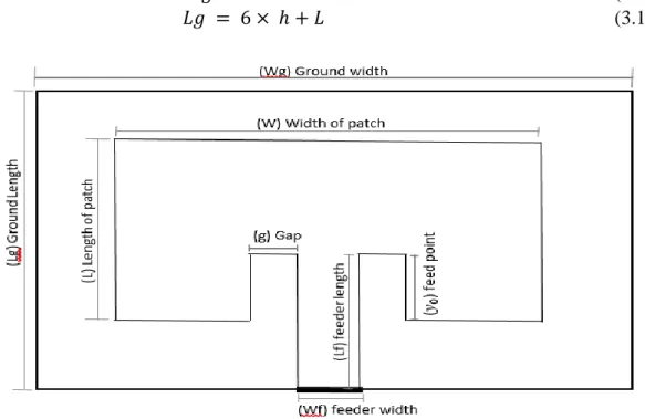
Where c is the light of speed, 𝑓_𝑟 is the resonant frequency and 𝜀_{𝑟𝑒𝑓𝑓} is the effective dielectric constant. The unit of length is in millimeters, therefore, the multiply with10−9.

H. Calculation of the ground plane dimensions [48]

𝑊𝑔 = 6 × ℎ + 𝑊 (3.17)

𝐿𝑔 = 6 × ℎ + 𝐿 (3.18)

(29)

4.2 Design analysis of Microstrip antenna

4.2.1 Selection of Material

In the antenna design the material selection is an important factor. Material with higher dielectric constant reduced size of the antenna, as shown in Equation (3.1, 3.2). FR-4 substrate is used for this design, its thickness is 1.55 mm (millimeter) and dielectric constant is 4.4. FR-4 is having high performance and low loss substrate. It is capable for multiple lamination cycles, lead free soldering and robust to standard PCB (Printed Circuit Board) processing. The circuit fabrication issued for the FR-4 is well defined and it has good reliability characteristics. PCB needs better thermal management and FR-4 have a thermal conductivity with a value of 02.5 W/m/k. FR-4 has a higher Df (Dissipation factor) 0.02 as compared to other frequency laminates. FR-4 material is used in many PCB applications with low cost and its performance is well defined [49].

4.2.2 Selection of Frequency

Microstrip antenna is designed in free space with 4 GHz frequency and this microstrip antenna is used as sensor.

Table 4 Microstrip Antenna parameters specifications

Specify Parameters of microstrip antenna

Frequency (𝑓_𝑟) 4 Ghz

Thickness of substrate (h) 1.55 mm Dielectric constant of substrate (𝜀𝑟) 4.4

Impdance (Z) 50 ohm

Calculate Parameters of microstrip antenna from equation 3.1 to 3.18 Width of Patch (W) 22.82 mm

Length of patch (L) 17.42 mm Feeding point (𝑦₀) 6.45 mm

Microstrip Line feeder Length (Lf) 4.65+6.45= 11.1 mm Microstrip Line feeder Width (Wf) 2.89 mm

Gap of microstrip line (g) 0.12 mm Ground Plane Length (Lg) 26.72 mm Ground Plane width (Wg) 32.12 mm

4.2.3 Selection of feed technique

4.2.3.1 Coaxial Probe

Microwave antenna consists of three layers. The top layer is the patch of antenna and use PEC (perfect electrical conductor) from CST with a thickness (h1) of 0.035 mm. The middle layer is the dielectric substrate with the thickness (h) of 1.55 mm. The lower layer is called ground plane. Figure 13, shows the microstrip antenna connected with SMA (Sub Miniature version A) connector. The SMA connecter is attached with the patch on location 𝑦₀ and W/2.

(30)

Figure 13 Microstrip Antenna with Coaxial Probe

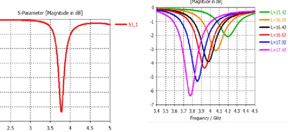
After calculation of all necessary parameters of microstrip antenna, shown in Table 4. The antenna is simulated in CST and then analyzed. The resonant frequency is 4 GHz, so frequency from 2 GHz to 5 GHz is chosen for simulation. The return loss of the microstrip antenna is -6dB at frequency 3.8 GHz, as shown in Figure 14a. Table 2 shows how much power is reflected and transmitted in specific return loss. -6dB means that 30 % of power is reflected and 70 % of power is transmitted. Good design antenna needs return loss below -10dB which will be a better antenna design.

Figure 14 Return Loss of Microstrip Antenna with Coaxial Probe

Figure 14a shows, the antenna gives response on 3.8 GHz which is not the desired frequency (4GHz). Figure 14b shows that decrease the length of antenna from L= 17.42mm to 16.42mm will give response on desired frequency. The return loss on length 16.42mm is -4dB which is not acceptable as a good antenna.

(31)

Figure 15 shows when increased the feeding location (𝑦₀) from 6.45 mm to 7.45 the return loss is decreased from -4dB to -10dB. The feeding location (𝑦0) 5.45 mm gives good response on

the desired frequency.

Figure 15 L=16.42mm, W=22.82 and Y0 from 5.45 mm to 7.45 mm

Figure 16 shows when the length of microstrip antenna is increased the return loss is below than -20db. After analysis of length (L) and feed location (𝑦₀), now we need to change the width of microstrip antenna. Figure 17 shows the width of antenna from 22.82 mm to 23.82 mm. The microstip antenna with configuration (L=18.42 mm, 𝑦₀ = 5.45 mm and W = 23.82 mm) return loss -40dB, as shown in Figure 17.

(32)

Figure 17 L=18.42 mm Y0 = 5.45 and W is change from 20.82 mm to 24.32 mm

Table 5 Different microstrip size antenna with Coaxial Probe feed technique

4.2.3.2 Microstrip line

The microstrip line consists of three layers. The top layer is patch of antenna whose material is PEC (perfect electrical conductor) from CST with a thickness (h1) of 0.035 mm. The middle

Design Number Parameters Retur n loss Figure Remarks Design 1st W=22.82mm L= 17.42mm 𝑦₀ = 6.45 mm

-6dB Figure 14a Original design.

Design 2nd

W=22.82mm L= 16.42mm 𝑦0 = 6.45 mm

-4dB Figure 14b Change parameter L to achieve the desire resonate frequency but return loss above -6dB compare design 1st. Design 3rd W=22.82mm L= 16.42mm 𝑦₀ = 5.45 mm

-10dB Figure 15 Change the feeding location to achieve good return loss compare 2nd design but the resonate frequency change from 4GHz toward 3.5 GHz Design 4th W=22.82mm L= 18.42mm 𝑦0 = 5.45 mm

-20dB Figure 16 Increase the length of design 3rd gives return loss -20dB which is good compare design 3rd. Design 5th W=23.82mm L= 18.42mm 𝑦₀ = 5.45 mm

-40dB Figure 17 Increase in the width from 2.84 mm to 23.82 mm gives return loss -40dB which is better from all pervious designs.

(33)

layer is the dielectric substrate having same size as the ground plane, the substrate thickness (h) is 1.55 mm. The lower layer is called ground, the ground plane also uses PEC. In this technique microstrip feed is connected from edge to the microstrip patch, as shown in Fgure 18.

Figure 18 Microstrip Antenna with Microstrip Line

The parameters of microstrip antenna (W, L, 𝑦₀, Wf, Lf, g , Wg, Lg) is shown in Table 4. The microstrip antenna is design in the CST which is shown in Figure 18.

The return loss of the microstrip antenna is -10dB at frequency 4 GHz, as shown Figure (19.a). This design needs more analysis to optimize the microstrip antenna. Figure (19.b) shows when changed the gap of microstrip line from 0.12 mm to 0.3 mm it gives return loss below than -25dB.

Figure 19 Return Loss of Microstrip Antenna with Microstrip Line

When the length is decreased from 17.42mm to 17.22mm, it gives response on the desired resonate frequency 4GHz but the return loss is above -25dB, as shown in Figure 20.

(34)

Figure 20 W = 22.82mm, y0= 6.45mm gap = 0.3 and L is from 17.12mm to 17.52 mm

The feed location is changed from 6.45 mm to 6.25mm it gives return loss below then -30dB, as shown in Figure 21.

Figure 21 W = 22.82mm, L=17.22mm, gap 0.3mm and Y0 change from 5.45 to 6745mm

Figure 22 shows that change in length (L) from 17.22 mm to 17 .50 mm gives return loss of -40dB.

(35)

Figure 22 W = 22.82mm, y0= 6.45mm gap = 0.3 and L is from 17.22mm to 17.50mm

Figure 23 shows that change of Wf and W does not effects, so Wf is 2.89 mm and W is 22.82 mm which is the final parameter for microstrip line antenna.

(36)

Table 6: Different microstrip size antennas with microstrip line feed technique

4.3 Design of Android Application

To Design the android application, we need to figure out the problem in the current system. The first question “How current system is working” and understand the current system architecture which is discussed in section “Related work and current working system”. The second question where the problem is in the current system and how we can solve that problem.

Problem in current System: - The current system has the following problems

a) The Patient’s data is saved in s1p file format. b) No central database to keep s1p files data.

c) Every time imports s1p file in VNA/J GUI or use Matlab [23]

d) There is no any specific application to convert s1p file data into database.

e) There is no any application that converts data (s1p data to database) and then show in android application.

f) There is no any specific android application for monitoring the healing bone of patient.

4.3.1 Requirement Engineering

The Requirement Engineering is the process to define the descriptions of the system, that how the system will work and how system will fulfill the customer needs. The requirements are high level abstraction statements which only describes that how the system will work. The

Design Number Parameters Retur n loss Figure Remarks Design 1st W=22.82mm L= 17.42mm 𝑦₀ = 6.45 mm g = 0.12 mm

-12dB Figure 19a Original design.

Design 2nd W=22.82mm L= 17.42mm 𝑦₀ = 6.45 mm g = 0.3 mm

-28dB Figure 19b Change parameter g gives -28dB which is good from design 1st_.

Design 3rd W=22.82mm L= 17.22mm 𝑦₀ = 6.45 mm g = 0.3 mm

-24dB Figure 20 Change parameter L to achieve the desire resonate frequency but return loss above -28dB compare design 2nd. Design 4th W=22.82mm L= 17.22mm 𝑦0 = 6.25 mm g = 0.3 mm

-32dB Figure 21 Change the feeding location (𝑦₀) from 6.45 to 6.25 mm gives good return loss compare 3rd. Design 5th W=22.82mm L= 17.50 mm 𝑦₀ = 6.25 mm g = 0.3 mm

-40dB Figure 22 Increase length (L) from 17.22 to 17.50 give better return loss. Change of W and Wf didn’t so much effect in this design, as shown in figure 23.

(37)

Requirement Engineering process is divided into two levels: user requirement and system requirement. The user requirement is the high level abstract requirement, for example “convert s1p file into database” this is the high level abstract where user does not know how to convert the s1p file into database. The system requirement is detailed description of what the system will do, for example the step involves how the S1P file will convert to database. Software system requirement are classified as functional and non-functional requirement [50].

Functional Requirement:

-

The functional Requirement of system describes the behavior of system that what the system should do, how system will work with the specific input. The functional requirement describe the user requirement in the form of system functions, its input and outputs, exceptions etc. [50]. The functional Requirement of the Android Application for monitoring long bone defects are described in the following section.

a) Convert S1P file data into Database: - The following steps are involved completing this requirement.

a. Collect the patient information from user. b. Select s1p file of the patient.

c. Read s1p file. d. Parsing the file data.

e. Extract specific information. f. Connect with database.

g. Save the patient data with extract information in centralize data base.

b) Create Web service: - Web service is software which is designed to run as server. It is dynamic and platform independent application which is used for exchanging data between applications or any system. For mobile devices web service is the way to exchange data with database or other system application. [51]–[54]. The following steps are involved to create web service

a. Connect with database. b. All patient list service.

c. Selected patient’s records date service. d. Selected patient’s measurement data service. e. Services Available to client

c) Connect Android application with web service: - Android application can communicate with database through the web service. To run android application, first we need to connect with web service.

d) Show all patients’ name in android application. e) Select patient from android application.

f) Select the patient’s measurement. g) Show patient’s measurement in graph. h) Show patient’s bone healing progress.

i) Setting of application: - set the minimum and maximum range for return loss. Set the reference limit for return loss with comments text. Set point on each measurement in the frequency.

(38)

Non-functional Requirement:

-

Non-functional requirements describes the functionality of the whole system, rather than the individual system services, it is the constraints or limitations of the whole system such as reliability, response time, performance, security, availability and store occupancy. Non-functional requirement is more critical than individual functional requirement. Functional requirement focuses only in the individual service, while the non-functional requirement describes the whole system, failing to meet a non-non-functional requirement can mean that the whole system is unusable [50] . Some non-functional requirements of the system is mentioned below.

a) Web service will be running 24/7 so that mobile application can communicate with web service.

b) The web service should be capable to handle maximum number of client request. c) Web service should respond to client request and web service should not fail in any

condition.

d) The android application should never fails in any condition. Android application should be robust.

e) The android application response time with web service should be minimal.

4.4 Proposed System

The working of current system is described in first chapter of section “Related work and current architecture” and the problem of current system is mentioned in fourth chapter. To solve this issues there was a need to develop a new system. The new system consists of three parts, window application which convert s1p file to database, web service which is running 24/7and android application which shows the patient’s data. Figure 24 shows the proposed system architecture concept which consists of three modules, the figure shows how the current system will integrate with proposed system and how the proposed system will work. First user will generate S1P file from Mini VNA, The first module is window application which parse S1P file and convert the file data into database. The second module is web services which takes data from database and make service and the third module is android application.

(39)

(40)

30

5 Development

5.1 Development of Sensor

The previous chapter provides the analysis of micro strip patch antenna. Table 5 shows that design 5th microstrip antenna (W= 23.82 mm, L = 18.42mm and 𝑦₀ = 5.45mm) is a good design with coaxial feed technique. Table 6 shows that design 5th microstrip antenna (W = 23.82mm, L =17.50mm, 𝑦0 = 6.25mm and g =0.3 mm) is the good design with mircostrip line feed

technique to take these two design for future analysis as sensor.

5.2 Long Bone (Femur, Tibia) Properties

The long bones of the legs are covered by complex organs like Muscles, Fat and skin. The outer organ of the leg is skin which is thin and covered with large hairs. The skin consists of main three layers: Epidermis, Dermis and hypodermis. Epidermis is the outer layer of the skin which consists of three cells squamous cells, Basal cells and Melanocytes. The minimum thickness of epidermis can be found in eyelids which are half a millimeter and the maximum thickness is 1.5 mm in the palms of the hands and soles of the feet. The dermis is the middle layer which consists of Blood Vessels, lymph vessels, hair follicles and nerves etc. The Dermis thickness of eyelids is 0.6 mm and the soles of feet are 3 mm. The overall minimum thickness of epidermis and dermis is 1 millimeter, while the maximum thickness is 4.5mm. The third layer of skin is hypodermis which consists of a network of collagen and fat cells. The minimum thickness of fat is 3.50mm and maximum thickness of fat is 13mm [56]–[60]. Long bone also have muscles with minimum thickness of 13 mm and maximum thickness of 25 mm [61].

Table 7 The Minimum and Maximum thickness of the Human organs

Organs Name Minimum value Maximum Value Skin 1 mm thickness 4.5 mm thickness Fat 3.5mm thickness 13 mm thickness Muscle 13mm thickness 25 mm thickness Bone 50 mm thickness 70 mm thickness

5.3 Antenna as sensor

The microstrip antenna from Table 5th and 6th can be used as sensor for measurement of defected long bones. For good sensor it is important that antenna is matched along with the long bone of human body. The antenna is simulated as sensor in CST studio and the human tissues like skin, fat, muscle and bone properties are used from CST studio library. The model is divided into four layers skin, fat, muscle and bone. The sensor will be attached to the first layer, which is skin layer. The skin layer covers the fat layer, fat layer covers the muscle and muscle layer covers the bone, the model is shown in Figure 25. These four layers complete the human model for long bone. The width and length of layers is 120 mm.

(41)

Chapter 5 Development 31

Figure 25 Sensor on Long bone model

InTable 5, it was found that design 5th_{is good antenna for Coaxial Probe technique, so the}

designed antenna was placed on long bone model and then simulated. The model consists of four layers, each layer thickness is the minimum value of the human organs from Table 7. The antenna gives response on 3.6 GHz in free space when placed the antenna on model then it gives response on 2.56 GHz but then return loss is above -4dB, as shown in Figure 26.

Figure 26 Return loss of coaxial probe sensor in Free Space and body model. (Antenna: - L=18.42 mm Y0 = 5.45 mm and W = 18.42mm) (Model: - skin thickness =1 mm, fat thickness= 3.5 mm, muscle thickness = 13 mm and bone thickness = 50 mm)

Figure 27 shows when changed the thickness of skin from 1 to 3.6 mm then the return loss is not below than -10dB, this antenna is not acceptable as sensor because the antenna is not matching with long bone model. The coaxial probe antenna did not give the good result as sensor.

(42)

Figure 27 Return loss of coaxial probe sensor to change thickness of skin. (Antenna: - L=18.42 mm Y0 = 5.45 mm and W = 18.42mm) (Model: - skin thickness change from 1 mm to 3.6 mm, fat thickness= 3.5 mm, muscle thickness = 13 mm and bone

thickness = 50 mm)

In table 6, it was found that design 5th is good antenna for microstrip line technique, so the designed antenna was placed on long bone model and then simulated. The antenna gives response on 4 GHz in free space, when this antenna is placed on model then it give response on 2.57 GHz and the return loss is below -10dB, as shown in Figure 28.

Figure 28 Return loss of microstrip line sensor in Free Space and body model. (Antenna: - L=17.52 mm Y0 = 6.25 mm, W = 22.82mm and g=0.3 mm) (Model: - skin thickness =1 mm, fat thickness= 3.5 mm, muscle thickness = 13 mm and bone

thickness = 50 mm)

When skin thickness is changed from 1 mm to 3.6 it provided the better results, skin thickness of 3mm provided good return loss which is below -60dB, as shown in Figure 29 (a). The fat thickness is changed from 4mm to 13mm. Fat thickness of 11 mm provided good return loss, as shown in Figure 29 (b), so for next simulation the fat thickness is kept 11mm

(43)

Figure 29 Return loss of microstrip line sensor to change thickness of skin. (Antenna: - L=17.52 mm Y0 = 6.25 mm, W = 22.82mm and g=0.3 mm) a) Model:- skin thickness change from 1 mm to 3.6 mm, fat thickness= 3.5 mm, muscle thickness =

13 mm and bone thickness = 50mm

Now need to optimize the sensor for muscle and bone layers. When changed in muscle and bone thickness its gives the same return loss. When changed dielectric constant of bone from 10 to 18 there is no change in simulation which mean that rectangular micro strip antenna do not detect the change of dielectric constant, so this type of antenna is not good as sensor, as shown in Figure 30. To detect long bone defect needs narrower bandwidth antenna which can detect small changes in dielectric constant.

Figure 30 Return loss of microstrip line sensor to change thickness of skin. (Antenna: - L=17.52 mm Y0 = 6.25 mm, W = 22.82mm and g=0.3 mm) Model: - skin thickness 3, fat thickness= 11 mm, a )muscle thickness change from 13 to 25 b) bone

(44)

The Microwave group of Uppsala University has designed SSR sensor for Skull under supervision of Prof. Robin Augustine which gives good result. Later the group optimized this sensor for long bone, the sensor is placed on cuboid and cylindrical model. The thickness of skin is 2 mm, muscle 25mm and bone 35mm [21], [62], as shown in Figure 31.

Figure 31 SSR Sensor on Long bone model [62]

When sensor is placed above the model in CST studio and then simulated, the normal (health bone) gives response on 2.2 GHz and the fractured bone gives response on 2.4 GHz so there is variation between frequency which is enough to determine the defected bone and the difference of this variation frequency can be used for healing analysis, as shows in Figure 32(a). When this senor is placed on square phantom the normal (health bone) gives response on between 2.3 and 2.4 GHz while fracture gives response on 2.5 GHz, as shown in Figure 32b.

(45)

Figure 32 Simulation and Phantom Result [62]

5.4 Development of Android application

The previous chapter described the propose system which consist of three modules. First we need to understand the current system and its requirement. The current system have s1p files which has contains different information. First step is to understand the s1p file and its information. S1P file has different fields but group was interested in three fields, frequency, s11 value and phase. The group also guides in requirement engineering which was discussed in previous chapter.

5.4.1 Module 1 Implementation

Convert file to data base: - After gathering information the next step is to analyze how to store the s1p file fields into database. Database is designed in SQL server, database consist on three tables patient records, measurement date and patient measurement. The database diagram is attached in Appendix. The implementation of parsing s1p file fields and then to store into database is done in C# visual studio.

(46)

With the help of user interface design user can enter patient’s record, patient’s measurement and also user can check patient’s information in software. For testing purpose few patients data was entered which was saved successfully in database, as shown in Figure 33.

Figure 33 software interface (add patient, insert patient measurement

5.4.2 Module 2 Implementation

Web service: - Web service is developed in the visual studio C#. The web service takes data from the database. Client request for some operation and web service performs operation and sent back the result in JSON (Java Script Object Notation). Web service has many classes like connecting with database, convert data into JSON and Get operations class, those classes are attached in Appendix. The Service is deployed on local IIS (Internet information Services) [63]. The local network can access this web service. Service is running in web browser to test that a service is located on network, as shown in Figure 34.

(47)

Figure 34 Web service on localhost

5.4.3 Module 3 Implementation

Android application: - This was the main part of the thesis. This is the front end of the system where user can see the information regarding return loss and frequency graph, the healing process, how much bone is healed. Application is implemented in Android studio. The user interface is designed in Android studio XML and code implementation is done in java. MPAndroid chart library is used for line graph and bar graph, this is good library for graphical data in android application, so for graphical interface this library is used [64]. Android application is tested on Samsung J5 (Android 5.1.1 API 22). Figure35 (a) shows Patient’s list from where user can select any patient. When user selects patient name then the corresponding patient’s measurement date will be shown in drop down list, as shown in Figure 35 (b). Figure 35 (c) shows the patient’s measurement graph and user can select anything from the menu bar like setting menu, patient records menu and healing progress.

(48)

(49)

Figure 35 (d) shows setting related to graph, user can fill the graph area by clicking on “Draw filled area”. When user clicks on “Draw circles” then on each value it will draw a small circle. User can also set the value of return loss, and then from that value graph will be displayed. User can also zoom in and out the graph, as shown in Figure 35 (e). The Figure 35 (f) shows the progress of healing, if bone is healed completely then value will be equal to “1”. If the healing value is below than “1” its means that healing progress will be continued.

The user can also select some basic setting like graph line width, graph area full color depth, reference measurement, as shown in Figure 36.