T-RFLP analyses of biocides influence on white water micro-organisms – planktonic and in biofilm

School of Sustainable Development of Society and Technology

T-RFLP analyses of biocides

influence on white water

micro-organisms – planktonic and in

biofilm

Rebecka Bodin

Degree Project, ECTS 30.0 At STFI-Packforsk AB Stockholm, 2008-06-11 Supervisor: Dr Ewa Lie Examiner: Professor Carl Påhlson

2

Acknowledgment

This work was carried out at STFI-Packforsk under the supervision of Doctor Ewa Lie. I would like to thank Ewa for all the help during this whole process. I would also like to thank all the people working at STFI-Packforsk for making me feel like “one of them”. The author would also thank Professor Carl Påhlson at Mälardalens Högskola for the encouragement and guiding.

Last but not least, a very special thanks to my colleagues, Sara Svensson, Therese Alm and Johanna Waltersson, for their friendship and support.

3

Abstract

When paper is manufactured, deposits often form in the machines. These deposits are slimelike and can interfere with the papermaking process. The slimelike deposits are aggregates of organisms, also known as biofilm. One single type of micro-organism can form a biofilm, but most biofilms consists of a mixture of several different kinds of micro-organisms and can form on about any conceivable surface. To control the aggregates of micro-organisms a slimecide is added, a so-called biocide. To examine what kind of bacteria that is included in the biofilm and also which bacteria that is killed or not killed by the biocide, Terminal Restriction Fragment Length Polymorphism analysis (T-RFLP) can be used.

In this report we examine biocides impact on biofilm produced in the laboratory.The biocides were first tested for possible interference with the PCR-step of the T-RFLP analysis. None of the tested ten biocides inhibited the PCR process the biofilm was formed on metal plates when these were lowered in a beaker with white water. Three different beakers were set up, one with addition of a biocide with active component 4,5-DICHLORO-1,2-DITHIOLONE from the start, one with the addition of the same biocide after three days and one with no addition at all of biocide. Samples were taken from the beakers and analyzed with T-RFLP.

In this report, we show that biocides affect planktonic and biofilm micro-organisms differently. There are however some micro-organisms in the biofilm that does not get affected by the biocide.

The experimental in this report is a good way of investigate the influence that biocides have on planktonic and biofilm micro-organisms, but to get even greater result the experiment should be done over a longer period of time and repeatedly.

4

Table of contest

2.1 Biocides effect on the PCR reaction... 11

2.2 White water and slime ... 12

2.3 Cultivation ... 12 2.4 Formation of biofilm ... 12 2.5 DNA-extraction ... 14 2.6 T-RFLP ... 14 2.6.1 PCR ... 14 2.6.2 Quantifying ... 16 2.6.3 PCR purification ... 16 2.6.3.1 MB Nase ... 16 2.6.3.2 E.Z.N.A. ... 17 2.6.4 Restriction digestion ... 17 2.6.5 Ethanol precipitation ... 17 2.6.6 Data analysis ... 17 2.6.6.1 Peak Scanner v.1 ... 17 2.6.6.2 Cluster analysis ... 18

3. Result and discussion ... 19

3.1 Biocides effect on the PCR reaction... 19

3.2 Cultivation ... 19

3.3 PCR ... 20

3.4 Quantifying of viable bacteria ... 22

3.4.1 Concentration in White water... 22

3.4.2 Concentration in Biofilm ... 23 3.5 Formation of biofilm ... 25 3.6 T-RFLP analysis... 26 3.6.1 Peak Scanner v.1 ... 26 3.6.2 Cluster analysis ... 30 4. Conclusions ... 32 5. References ... 33 Appendix I ... 35 Materials ... 35 Chemicals ... 36 Appendix II ... 37

5

1. Introduction

When paper is manufactured, microbiological deposits sometimes form in the machines. These deposits are slimelike and can interfere with the papermaking process. The interference might give the paper a wrong nuance, break the paper web or give the paper spots and dots. The paper can also get a repulsive odour [10, 12]. Another aspect is that if there are too much microbes in the paper or board used for food packages, the paper cannot be used. Also the machine can have major trouble if the there is too much slime and it can get to the point where the machine has to be stopped for cleaning. Bacteria on the surface of the machine may also cause corrosion [9, 10].

These slimelike deposits are aggregates of micro-organisms and they often starts as biofilms. Biofilm is formed because of the favourable environment that exists during the papermaking process such as warm water (30-50 ºC) with the right pH (5-8) and lots of nutrients, i.e. from cellulose and starch. This phenomenon has also been noted in earlier studies [4, 8, 10, 11, 16, 17]. For the papermaking process, bacteria that are attached in a biofilm are more troublesome than if they are swimming freely. However, there are paper machines that work without trouble in spite of the count of planktonic bacteria is over 106 CFU mL-1 [8].

Figure 1. Photographs of biofilms that have grown on surfaces in the splash areas of the wet-end part of a paper machine (A-C) [8].

Since these aggregates of micro-organisms influences the papermaking process negatively, often a slimecide is added, so-called biocides. The biocide kills off the micro-organisms, but does not have any impact on the process. Earlier studies have however shown that biocides do not kill off micro-organisms in a biofilm effectively enough and that biocides is often more effective against platonic cells t [21, 24, 25].

6 To examine the bacteria included in a biofilm and also to examine biocides impact on bacteria, a good technique is required. One technique that has been used with success to follow bacterial composition is Terminal Restriction Fragment Length Polymorphism analysis (T-RFLP) [2, 5, 7, 14, 18, 23]. This technique does not require any cultivation of the sample and is therefore a very useful method since many bacteria is uncultivable.

1.1 Biofilm

Biofilm is an accumulation of micro-organisms that grows on a firm substance and has a complex shared structure. The structure both protects the micro-organisms and allows them to grow. The aggregation of a biofilm begins with the affixation of planktonic micro-organisms to a surface. The micro-organisms attach to the surface by excreting a slimy, glue-like substance (Fig 2). Biofilms can form on about any conceivable surface, such as metals, plastics, natural materials, medical implants, kitchen counters, contact lenses, the walls of a hot tub or swimming pool and human and animal tissue. Wherever there is moisture, nutrients, and a surface biofilms will presumably be established. [8, 25, 26]

One single type of micro-organism can form a biofilm, but most biofilms consists of a mixture of several different kinds of micro-organisms. Biofilm can also consist of fungi, algae, yeasts, protozoa and non-living debris. Some micro-organisms cannot attach to a surface by them self, but if another micro-organism attach first they can attach to them. In that manner micro-organism that do not have an attaching ability can be a part of a biofilm. [8, 19, 26]

Engineers and scientists have discovered that biofilms are held together by extracellular polymeric substances or EPS. [1, 8, 21] The cells produce strands of EPS and are held together by these strands. This indulge the cells to build up a complex, three-dimensional, attached community that are resistant to attacks that would extinguish individual cells that are not a part of a biofilm. [8, 19, 26]

7 When bacteria are a part of a biofilm they are more resistant to antimicrobial agents than if they are in their planktonic state. This is caused by the fact that bacteria properties, for example attachment ability, changes within the biofilm since the protected and compact environment gives them the opportunity to collaborate and interact in different ways [8, 12]. Biofilm becomes in this way very hard to fight off, antimicrobials can only kill the bacteria on the surface of the biofilm and if the biofilm gets too thick the antimicrobials have no chance to penetrate and kill the bacteria within the biofilm.

1.2 Biocides

A biocide is a chemical substance that has the capability of killing different forms of living organisms. Biocides can target different kind of organisms and is therefore divided into two key areas:

 Pesticides, which includes fungicides, herbicides, insecticides, algaecides, molluscicides, miticides and rodenticides.

 Antimicrobial, which includes germicides, antibiotics, antibacterials, antivirals, antifungals, antiprotozoals and antiparasites.

Biocides can also be classified by their substances [20] and there are:

Alcohols: They are colourless volatile liquids that are effective without leaving

residues. Alcohols work fast but only in high concentrations and are more effective on Gram-negative bacteria than Gram-positive. Alcohol does not kill off spores.

Aldehydes: Get its antimicrobial effect due to that the aldehyde group is polar.

Oxygen pulls the electrons in the carbon-oxygen bond towards itself creating a electron inadequately at the carbonyl carbon atom which gives them the chance to react with nucleophilic cell entities. Aldehydes have the ability to kill of many different kinds of microbes due to their mechanism, including viri and spores.

Formaldehyde releasing compounds: These biocides can vary in property. They can

be solids or liquids, soluble in oil or soluble in water, scentless, alkalic, neutral or somewhat acidic. These compounds give the opportunity to use the active agent, formaldehyde, without worrying about its inexpedient features.

Dimethoxane: A biocide that is very useful against yeast, bacteria and fungi.

Dimethoxane can be mixed with water and is highly soluble in organic solvents and oils.

Phenolics: Also known as carbolic acid. This is a toxic, colorless crystalline with a sweet tarry odor and is a membrane-active microbicides.

Acids: These are in general good against animalcules and belong to the

membrane-active substances. Acid often have their antimicrobial effect when they are in their undissociated state and can penetrate the cell membrane.

8

Carbonic acid esters: Dimethyl dicarbonate and halogens that contain esters have

electrophilic character which make them able to react with nucleophilic groups on the microbes and in that way make them a very effective bactericidal.

Amides: Belongs to the membrane-active microbicides. Usually carbonic acid amides

do not have microbicidal effects. To get antimicrobial aliphatic carbonic acid amides, toxic groups or structural elements have to be added.

Carbamates: Esters and salts of carbamic acids belong to carbamates, but these

kinds of microbicides are very diverse in their effectiveness and mechanisms of activity.

Dibenzamidines: These substances belong to the membrane-active microbicides and

are used as antiseptics, but are sometimes also used as preservatives for cosmetics.

Pyridine derivatives and related compounds: Also belongs to the membrane-active

microbicides, but have chelate features.

Azoles: Azoles are fungicides with low ecotoxicity and work by blocking the

biosynthetic reactions in the reformation of lanosterol to ergosterol.

Heterocyclic N,S compounds: Examples of these compounds are thiazole and

isothiazole and they are cyclic organic microbicides carry N and S in the ring.

N-haloalkylthio compounds: The bactericidal influence of these compounds lies in the

capability of the N-S bond to open and react with nucleophilic elements of the microbial cell.

Compounds with activated halogen groups: The activity of these microbicides comes

from reaction between the positive carbon in these compounds and nucleophilic units of the microbial cell.

Surface active agents: Surface active agents antimicrobial activity is symbolized by

their capability to lower the surface tension of aqueous fluids. This allows them to work as emulsifying agent, detergents and wetting agents. There are two kinds of these microbicides, one is hydrophobic and the other one is hydrophilic.

Organometallic compounds: The most known organometallic compounds that are

widely used for material protection in large scale are organomercery and organotin. However these compounds may probably not be used as widely in the future because of their high ecotoxicity.

Various compounds: These compounds have antimicrobial effects but do not fit in

any of the other classifications.

Oxidizing agents: These compounds are very aggressive against micro-organisms

because of their strong oxidation power. This makes them unselective and encloses both Gram-positive and Gram–negative bacteria, fungi, yeasts, algae, spores and viruses.

9 All biocides that are used in Sweden or another EU country have to be passed on according to the Biocides Directive 98/8/EC. There the approved active substances are listed in Annex I.

Biocides are frequently used against micro-organisms to prevent biofilm forming and also in the papermaking industry. This is a must since biofilm can be a big economic loss, but repeated use of some biocides can cause resistance among the bacteria in the biofilm. The biocide becomes neutralized by the components in the biofilm more rapid than it can disperse into the biofilm [8, 24].

1.3 T-RFLP

T-RFLP is a method based on variation in the 16S rRNA gene where complex microbial communities, are studied. The T-RFLP method is a very good technique to analyze these mixed bacterial communities because it is culture independent, rapid, sensitive and does not need any genomic sequence information. The T-RFLP technique was at first elaborated for characterizing bacterial communities in samples with many different species. The technique has also proven to be applicable when characterizing fungi and bacteria in soil, therefore is T-RFLP widely used for that kind of analyses [2, 5].

In T-RFLP, DNA is amplified using fluorescent labeled primers in the PCR. The PCR products are then digested using restriction enzymes and the labeled fragments thus formed are then visualized with a DNA sequencer (Fig. 3). To analyze the result one could either just look at the electropherogram “peaks” or compare the results with a T-RFLP database with known species. Different species will have different terminal fragments length due to variety in the occurrence and location of the cutting sites. [5, 6, 14, 18].

The method can be divided in five keys steps [5, 27] that have to be completed (Fig. 3). These steps are;

 DNA isolation and extraction, which is often performed with a suitable kit.  PCR amplification of the 16S rRNA gene using fluorescently-labelled primers  Restriction enzyme digestion of the PCR product.

 Separation and detection of the digested products using electrophoresis.  Detection of the fluorescent fragment profile for each sample.

 Clustering analysis based on the outline of samples from step 4. Clustering analysis is then based on the outline of samples from step 5.

10

Figure 3. Schematic figure of the major steps in T-RFLP [27].

T-RFLP is proposed to be more sensitive when identifying fungi than Denaturing Gradient Gel Electrophoresis (DGGE) and that it cost less than using clone libraries, but both DGGE and clone libraries have some advantages that T-RFLP does not have. One way could be to use the techniques combined with each other to get the best results [5].

There can be some difficulties with the use of T-RFLP and other molecular methods such as efficient extraction of DNA, PCR amplification of target gene and that the peak-profile works on the assumption that a single peak represents one specific species [5 ,15].

1.4 Aims of the study

The aims of this study were:

A) To examine if biocides interfere with the PCR reaction, since earlier trials had shown possible inhibition with poor yield of DNA and one concern was that the biocide interfered with the PCR. If interference was detected the continuation would to investigate the action of the inhibition and how to adjust the problem.

B) If, however, there were no interference the aim were to look at how the biocide affected planktonic micro-organisms in white water and also biofilm formed in the white water. One important question is to get a better understanding of the start of biofilm formation.

C) Additionally question formulation and aim was if there were any differences if the biocide were added from the start or after a couple of days.

11

2. Materials and methods

Chemicals and materials that are used are listed in appendix I.

2.1 Biocides effect on the PCR reaction

To investigate if biocides interfere with the Polymerase Chain Reaction (PCR) a test was carried out. The test implicated ten different biocides (Table 1) that were each added to a PCR mixture, described in 2.6.1 with DNA extracted from a pure culture of

Bacillus cereus. The concentration of the biocides was 100 parts per million (ppm).

Table 1. Active components of the biocides that were used.

No. Active component

1. 3,5-Dimethyl-tetrahydro-1,3,5-2H-thiadiazine-2-thiono 2. 2,2-Dibromo-3-nitrilopropionamide 3. 2-Bromo-2-nitro-propane-1,3-diol 4. 4,5-Dichloro-1,2-dithiolone 5. 5-Chloro-2-methyl-4-iosothiazolin-3-one and 2-methyl-4-isothiazolin-3-one 6. Pentane-1,5-dial 7. Methylene bisthiocyanate 8. N-Alkyl-N,N-dimethyl-N-benzylammonium chloride 9. Di-n-decyl-dimethylammonium chloride 10. 1,2 bensoisotiazolin 3-one

When the biocides had been added to the PCR mixture the samples was placed in the Thermal Cycler and run with following PCR program.

94 C 2 min

25 cycles with 94 C 45 sec, 59 C 45 sec, 72 C 45 sec 72 C 10 min

The PCR conditions had been optimized in advance [7] to get the best results and are also used in latter experiments.

To analyse the effect of the biocides, the PCR products were checked on an ethidiumbromide-stained gel that was run with electrophoresis at 100 V for 45 minutes. This would show if the samples with biocides gave another intensity on the gel, than the positive control with no addition of biocide. If the biocide interfered with the PCR, the expected result, would be that the intensity of the fragment bands would be lower i.e. an inhibition had occurred.

12

2.2 White water and slime

In the experiments, white water and slime from a Swedish paper mill that manufacture board, is used. Five litre of white water had been taken from the bottom of the side aisle and had a pH of 7.4 and a temperature of 43 ºC. When the water arrived, within 24 hours after sampling, it was stored at 4 ºC until it was used. Slime had been collected from two places in the paper mill. Slime 1, was taken from a suction box and slime 2 was taken from a shake sieve. The slimes arrived at the same time as the white water, also within 24 hours after sampling, and were kept at 4 ºC until it was used.

2.3 Cultivation

The concentration of bacteria in white water was determined by cultivation on agar plates. The agar that was used was made of Tryptone Glucose Extract Agar (TGEA). A serial dilution of the white water was made from 1:1 to 1:10, 1:100, 1:1000 and 1:10 000 with Ringer solution. 50 µL of each dilution was spread out on two plates and then incubated over night in 37 ˚C. The colonies were then counted after two days and the bacteria concentration in the water could be determined.

To see which biocide that was going to be used in the white water cultivation inhibition tests with the water was again made, but this time shreds (Fig.7), which had been prepared with 50 µL of each biocide, was placed on the plates. All ten biocides were tested (Table 1).The plates were then incubated in 37˚C over night. The decision of which biocide that was going to be used was made on the effect that the biocide had, how big the “killing zone” was (Fig.7).

To validate how many bacteria the chosen biocide then killed off, cultivation on two TGEA-plates were made. This was performed with 50 µL white water containing 1 ppm of chosen biocide spread on each plate, and then the plates were incubated at 37˚C over night.

2.4 Formation of biofilm

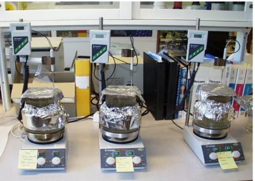
To investigate the bacteria that cause biofilm in the paper mill machines, biofilm had to be produced. This was done as followed. Three beakers where filled with one litre each of white water. Each beaker was placed in a water bath that then was positioned on a heater with agitation. The water bath worked in that way as a mantle to the beaker. A temperature control device was placed in the water and the temperature was set to 45 ˚C. (Fig. 4) To one of the beakers 1 ppm of biocide was added from the start and was named “red”. Another beaker got 1 ppm of biocide added after three days and was named “green”. The third beaker contained only white water and was named “blue”. The two beakers that had additament of biocide got a restock of 1 ppm of biocide each day. In each beaker seven stainless steel plates were placed. (Fig. 5) Before positioned in the beaker, the plates had been carefully cleaned, first with 99.5 % ethanol, then in an ultrasonic bath and finally autoclaved. Since about 100 mL of the white water evaporated each day, the beakers were refilled with 100 mL new white water each day.

13

Figure 4. Biofilm formation, the three beakers in position.

Figure 5. The stainless steel plates in the beaker with white water.

After day one, a metal plate from each beaker was taken out. The plates were air dried and then weighed. After weighing, the plates were each placed in a centrifuge tube, which then was filled with 35 mL MilliQ water. The tubes were positioned in an ultrasonic bath and ran for 40 minutes. Subsequently the tubes were centrifuged for 40 minutes at 13 000 revolutions per minute (rpm). The supernatant was disposed of and the pellet was used for further DNA-extraction. This process was repeated each day for four days, then again after seven days for three days.

Samples of 25 mL from each of the beakers were also taken for DNA-extraction from planktonic bacteria. The samples were centrifuged for 40 minutes at 13 000 rpm and the supernatant were then disposed of.

14 Bacteria that was growing on the inside of the beaker, after nine days, was collected with an inoculation loop and spread out on a TGEA-plates. The plates were then incubated over night in 37 ºC. The colonies was scraped off and used for DNA-extraction.

2.5 DNA-extraction

To characterize the bacteria with T-RFLP the DNA needed to be extracted from the samples. DNA in the white water, slime and the biofilm were extracted with the aid of an extraction kit for soil. The process was carried out according to a protocol that had been made from an earlier report [7].

Cultivated bacteria from the beakers were scraped off and extracted according the manufacturers protocol for DNeasy® Tissue.

2.6 T-RFLP

2.6.1 PCR

After the DNA-extraction the samples were amplified with PCR. This was carried out with the use of universal bacterial primers that gave a fragment of 920 base pairs (bp).

The PCR mixture for one sample contained following components, 0.5 µL of each primer 8fm (5'-AGA GTT TGA TCM TGG CTC AG-3') and 927r (5'- CCG TCA ATT CCT TTR AGT TT-3'), the forward primer had in advance been fluorescently 5' end labelled with 6-FAM, 2.5 µL PCR-buffer, 2.5 µL BSA, 1.25 µL dNTP-mix, 3.0 µL MgCl2, 0.25 µL rTaq polymerase and 0.5 µL template. To obtain the final volume of 25 µL, sterile MilliQ water was added. A positive and a negative control was also included, the positive with B. cereus and the negative with MilliQ as template.

The result from the PCR was then envisaged by gel-electrophoresis, which was run at 100 V for 45 minutes, and should show fragments band of about 920 bp if the PCR and extraction had been successful. Since there were too many samples for one gel the samples were split up on four.

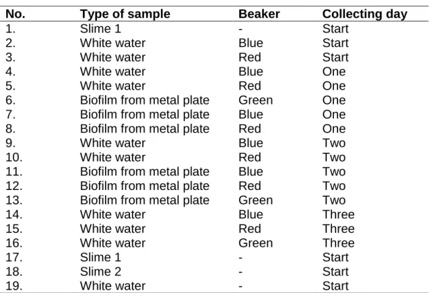
On the first gel 19 samples were run and the type of sample, which beaker and which day they were collected are listed in Table 2.

15

Table 2. Contents of the 19 samples on the first ethidiumbromide-stained gel, from which beaker the samples were collected and on which day.

No. Type of sample Beaker Collecting day

1. Slime 1 - Start

2. White water Blue Start

3. White water Red Start

4. White water Blue One

5. White water Red One

6. Biofilm from metal plate Green One

7. Biofilm from metal plate Blue One

8. Biofilm from metal plate Red One

9. White water Blue Two

10. White water Red Two

11. Biofilm from metal plate Blue Two

12. Biofilm from metal plate Red Two

13. Biofilm from metal plate Green Two

14. White water Blue Three

15. White water Red Three

16. White water Green Three

17. Slime 1 - Start

18. Slime 2 - Start

19. White water - Start

The second gel contained the next 18 samples, which are listed in Table 3.

Table 3. Contents of the 18 samples on the second ethidiumbromide-stained gel, were the samples was collected and on which day.

No. Type of sample Beaker Collecting day

20. Biofilm from metal plate Red Four

21. White water Blue Seven

22. White water Red Seven

23. White water Green Seven

24. Biofilm from metal plate Green Seven

25. Biofilm from metal plate Blue Seven

26. Biofilm from metal plate Red Seven

27. White water Blue Eight

28. White water Red Eight

29. White water Green Eight

30. Biofilm from metal plate Green Eight 30. Biofilm from metal plate Blue Eight

31. Biofilm from metal plate Red Eight

32. White water Green Nine

33. White water Red Nine

34. White water Blue Nine

35. Biofilm from metal plate Green Nine

36. Biofilm from metal plate Red Nine

16

Table 4. Contents of the nine samples on the third ethidiumbromide-stained gel, were the samples was collected and on which day.

No. Type of sample Beaker Collecting day

37. Biofilm from metal plate Red Three

38. Biofilm from metal plate Green Three

39. Biofilm from metal plate Blue Three

40. White water Blue Four

41. White water Red Four

42. White water Green Four

43. Biofilm from metal plate Green Four

44. Biofilm from metal plate Blue Four

45. Biofilm from metal plate Blue Nine

On the fourth gel the cultivated bacteria from the beakers were run and their information is listed in Table 5.

Table 5. Contents of the three samples on the fourth ethidiumbromide-stained gel, were the samples was collected and on which day.

No. Type of sample Beaker Collecting day

46. Biofilm from beaker Blue Nine

47. Biofilm from beaker Red Nine

48. Biofilm from beaker Green Nine

2.6.2 Quantifying

DNA-quantification was performed with a spectrofluorometer to see how much DNA the samples included.

On a 96-well plate, 98 µL TE was added to each well that was going to be used including a blank sample. Thereafter the samples were added, 2 µL PCR-product and 2 µL TE, as the blank sample. To each of the wells 100 µL PicoGreen solution were added. Then the plate was placed on a rotating table with tin foil over, to protect from light, and incubated for 6 minutes.

The plate was positioned in the spectrofluorometer and analyzed with the excitation wavelength set at 500 nm and the emission wavelength at 525 nm.

2.6.3 PCR purification

2.6.3.1 MB Nase

To get rid of single-stranded ends the samples were run in the Thermal Cycler with mung bean nuclease. 10 µL PCR-product of each sample was mixed in PCR-tubes with 34.75 µL MilliQ, 5 µL buffer and 0.25 µL MB Nase and then run for 90 minutes at 37 C in the Thermal Cycler.

17 2.6.3.2 E.Z.N.A.

When the samples had been digested with MB Nase they were purified with E.Z.N.A. Cycle-Pure Kit, following the manufactures protocol.

2.6.4 Restriction digestion

The purified products were digested with the restriction enzyme HhaI. 24µL purified PCR-product was mixed in PCR-tubes with 64 µL MilliQ, 2 µL HhaI and 10 µL buffer, which in this case was 10 × M Buffer. The PCR-tubes were placed in the Thermal Cycler and run with following program.

37 C 480 min 70 C 15 min

2.6.5 Ethanol precipitation

The DNA in the digested products were precipitated by adding 5 µL 3M NaAc and 100 µL ice-cold 99.5% ethanol and then incubated in – 20 ºC for a couple of hours. Thereafter the samples were centrifuged for 20 minutes at 20 000 rpm and the supernatant were disposed of. To wash the samples, 100 µL 70% ethanol was added and then the samples were centrifuged again for 20 minutes at 20 000 rpm. The supernatant was disposed of and the pellet was left to air-dry in 37 ºC until all fluids were gone. The pellet was then resolved in 30 µL of MilliQ water.

The samples were then sealed and marked to be sent to Labmedicin, Universitetssjukhuset MAS (Malmö, Sweden) for analysis. There the samples were analysed with an ABI 3730 DNA Sequencer and the standard marker that were used was GeneScan(tm) 600LIZ® size Standard with following fragment sizes:

20, 40, 60, 80, 100, 114, 120, 140, 160, 180, 200, 214, 220, 240, 250, 260, 280, 300, 314, 320, 340, 360, 380, 400, 414, 420, 440, 460, 480, 500, 514, 520, 540, 560, 580 and 600 bp.

2.6.6 Data analysis

2.6.6.1 Peak Scanner v.1

When the samples had been analyzed on the ABI 3730 DNA Sequencer, the raw data was transferred to Peak Scanner v.1. In Peak Scanner, following adjustment to the tuning was made before the samples were analyzed. The sample type was set on “sample”, the size standard was set on “600LIZ”, that had been created and added to Peak Scanner v.1 in advance, and the analysis method was set on “sizing default”,

18 that work on the assumption that the primer have not been removed from the samples. After the adjustment the samples could be analyzed and an electropherogram was created for each sample.

2.6.6.2 Cluster analysis

Cluster analysis was used for grouping the samples and is based on the distance between the samples and was performed in the statistical program R (www.r-project.org/). Two approaches were applied, quantitative, Bray-Curtis index, where the absence and presence of the peaks in the electropherogram is considered and qualitative, Sorensen´s index, where the peak area as well as absence and presence of the peaks are considered.

19

3. Result and discussion

3.1 Biocides effect on the PCR reaction

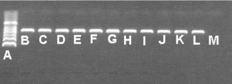
When the samples with biocides had been run with the Thermal Cycler the result was visualized on an ethidiumbromide stained gel (Fig. 6).

Figure 6. Fragments, on an ethidiumbromide stained gel. A: gene ladder 100bp, B – K: biocide nr.1 – 10 (Table 1), L: positive control and M: negative control.

Comparing the lanes at the gel, there seems to be no indication that the biocides interfere with the PCR process. The bands from the samples containing biocide (Fig 6: B – K) have the same intensity as the positive control (Fig. 6: L). If the biocides would have had any negative effect on the PCR reaction the expected result would be that the band should have a lower intensity and this could not be detected. With this in mind, the following experiments could be done without the risk for negative interference by the used biocides on the PCR reaction.

3.2 Cultivation

Cultivation of the white water gave countable colonies on the plates with the dilution 1:1000 and 1:10 000. This gave a bacteria concentration of, 8.5 × 105 bacteria per mL white water for the 1:1000 dilution and 8 × 105 bacteria per mL white water from the 1:10 000

The effect of the biocides in Table 1 was tested on discs on undiluted white water. The agar plates were observed after one day incubation and the biocide with the biggest killing zone was the one used in the further experiments. It was obvious, when looking at the plates (Fig. 7), which biocide that had the best killing ability, i.e. biocide number 4, 4,5-DICHLORO-1,2-DITHIOLONE. This result was not totally unexpected since this biocide has been shown to be particularly effective against slime forming micro-organisms [20] with a Minimum Inhibition Concentrations, MIC, of 1 mg/litre nutrient solution. It is also a biocide that is used in pulp and paper mills and cooling water systems.

20

Figure 7. Pictures of the killing zone created by biocides that had been added on discs that were placed on agarplates.

To further investigate the chosen biocide it was added directly to the white water in a concentration of 1 ppm and the contact time was two hours before plating. The cultivation showed no growth after one day. The agar plates were therefore incubated for another day. After two days there were four colonies of the undiluted sample on one of the plates and on the other one there were ten colonies. The plates were then placed again in the incubation cabin. The plates were observed over the following couple of days but no more colonies were observed. The bacteria concentration could therefore be established to be 50 bacteria per mL white water and the killing ability for this biocide considered being very effective i.e. from 8 * 105 to 5 * 101cfu/ml.

3.3 PCR

When all the samples, from all three beakers, had been amplified the result was visualized on an ethidiumbromide-stained gel.

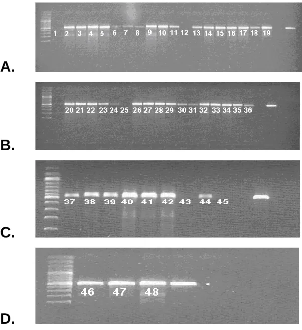
The result from the all of the gels is shown in Figure 8. On the first gel (Fig.8A) two samples did not show a fragment band. This was samples number 1 and 12 (Table 2). This could be caused by the absence of DNA in the sample. Another explanation is that the amount of DNA is too little to be visualized on the ethidiumbromide stained gel. A third aspect is that the samples have been contaminated so the DNA have been damaged and is therefore not showing any band. Some samples show a very weak band and this can be due to a low DNA concentration. The second (Fig.8B) and third gel (Fig.8C) also showed samples without fragment band. The explanation

21 to this can be the same as for the samples on the first gel. The fourth gel (Fig.8D) however gave nice strong bands for all three samples.

A.

B.

C.

D.

Figure 8. DNA fragments on an ethidiumbromide stained gel.

A: From the left: gene ladder 100bp, sample 1 – 19 (Table 2), negative control and positive control. B: From the left: gene ladder 100bp, sample 20 – 36 (Table 3), negative control and positive control. C: From the left: gene ladder 100bp, sample 37 – 45 (Table 4), negative control and positive control. D: From the left: gene ladder 100bp, sample 46 – 48 (Table 5), positive control and negative control.

22

3.4 Quantifying of viable bacteria

3.4.1 Concentration in White water

To get a measurement on the growth of planktonic bacteria in the beakers, quantification was performed with spectrofluorometer. This gave the concentration of DNA and a comparison between the different beakers. The main drawbacks with this method are the relative large contribution of nucleotides, single-stranded nucleic acids and proteins in the same reading range. Then there is the problem with interference caused by contaminants and the incapacity to distinguish between DNA and RNA. But with sensitive fluorescent nucleic acid stains, the problem can be circumvented.

The concentration values from the spectrofluorometer had to be adjusted since the samples had been diluted. This was done by multiplying the values with 100 due to the dilution of 100.

White Water

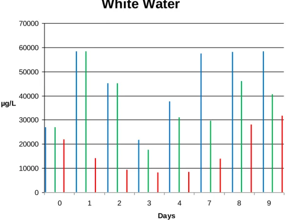
Figure 9. The DNA concentration in the white water from the three different beakers on the collecting day. The blue bar represent the blue beaker (control), the green bar represent the green beaker (biocide added after 3 days) and the red bar represent the red beaker (biocide added from start).

The concentration DNA in beaker blue and green were equal at the start, while it was a bit lower in the red, which indicates that the biocide was active and had killed of some micro-organisms in the red beaker. After day one the concentration increased

23 in both blue and green beaker and decreased in the red. This result is as expected since the biocide in the red beaker is killing micro-organisms and the concentration is therefore decreasing. Also the increase of concentration in the other two beakers is anticipated since the conditions are favorable for growth. After day two the concentration in all three beakers decreases. For beaker red this is expected and wanted, but for beaker green and blue it is a bit unexpected. One explanation to this phenomenon could be that the amount of bacteria in beaker green and blue got too large and begun to die since the nutrition depleted. Day three the concentration in all of the beakers further decreased, and once again this is expected for beaker red but not for blue and green (Fig. 9). This could be due to nucleotides, single-stranded nucleic acids and proteins that figure in the same reading range.

When looking at the concentration on day four it showed an increase in beaker blue and green and stayed about the same in the red. This could make more sense if it was not for the fact that beaker green now had the addition of 1 ppm of biocide and should have a decreasing concentration. Day seven, eight and nine the concentration in beaker blue had increased to a quite high level and this result is more favorable. In beaker red the concentration also increased during these days. This could be due to the absence of additament of biocide during day five and six and therefore the bacteria had the opportunity to establish themselves. Another aspect is that if a biocide is to be used it has to have a relatively quick degradation time and therefore the effect of the biocide is undermined, giving the micro-organism chance to grow. The result for beaker green during these days is not what was expected, the prediction would be that the concentration should decrease after the addition with biocide not the reverse.

However, the relation between green, blue and red beaker when comparing only one day at a time make sense. That is: for the first three days the blue and green beaker has the same amount of DNA while the red beaker with added biocide has less DNA. From the third day the DNA content in the green beaker (where now biocide is added) is less than in the blue beaker.

3.4.2 Concentration in Biofilm

The assessment of the DNA concentration in the biofilm on the metal plates gave an indication that the handling of the samples at the quantification may have caused poor results. This since many of the values gave a negative value and others a very low (Fig. 10). Looking at the handling of the samples there are three major drawbacks that probably led to the poor results. Firstly, collecting the plates from the beakers. At this stage some micro-organisms could have fell off leading to a lower concentration. Secondly, during the ultrasonic bath it is possible that not the entire sample came off, which also leads to lower concentration. And thirdly, there were only one plate per sample. Another aspect to keep in mind is that the amount of the samples was very low to begin with. One speculation about the beaker green showing rather high DNA content during the two last days is that the biocide addition has not been enough to kill the bacteria, but instead triggered the biofilm formation.

24 Metal Plates -1000 0 1000 2000 3000 4000 5000 6000 1 2 3 4 7 8 9 Days µg/L

Figure 10. The DNA concentration on the metal plates from the three different beakers on their collecting day. The blue bar represent the metal plate from the blue beaker (control), the green bar represent the metal plate from the green beaker (biocide added after 3 days) and the red bar represent the metal plate from the red beaker (biocide added from start).

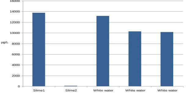
The evaluation of the concentration from the two different slimes and the white water gave that slime 1 and the three white water samples had approximately the same concentration. Slime 2 however showed a very low concentration, this is probably because a failure in the extraction process since it is not likely that slime have this low concentration of DNA (Fig. 11).

0 2000 4000 6000 8000 10000 12000 14000 16000

Slime1 Slime2 White water White water White water µg/L

Figure 11. The DNA concentration in the two slimes and in three samples of the same white water at the arrival.

25

3.5 Formation of biofilm

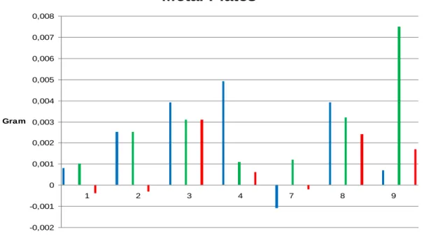
After the plates were removed from the beaker, the metal plates were air dried and then weight before DNA quantification and T-RFLP measurements (Fig. 12). The plates were weighed as a measurement of the formation of biofilm. The assumption was that the weight of the metal plate should increase the more biofilm that had been formed. Metal Plates -0,002 -0,001 0 0,001 0,002 0,003 0,004 0,005 0,006 0,007 0,008 1 2 3 4 7 8 9 Days Gram

Figure 12. The weight of the metal plates from the different beakers at the collecting day. The blue bars represent the metal plates from the blue beaker (no biocide added), the green bars represent the metal plates from the green beaker (biocide added after three days) and the red bars represent the metal plates in the red beaker (biocide added from start).

In the beaker that had no additives of biocide, (blue), the weight of the plates increased the first four days. After seven days the weight decreased remarkable, to then increase the day after and then again decrease. That the weight increased the first days was expected and hoped for, since the conditions in the beaker were optimum for the growth of micro-organisms and further to create a biofilm. But that the weight then decreased was at first a setback. The hope was that the weight should continue increase during the whole experimental.

The metal plates from the red beaker, that contained 1ppm of biocide 4,5-DICHLORO-1,2-DITHIOLONE, weighed less than from the beginning. This could be that the plates were not completely dried when they were first weighed. But it can also indicate that the biocide have killed of micro-organisms. After day three the weight had increased a lot and one can wonder if this measurement really should be reckoned. Something can have gone wrong, or the biocide has not had the impact that it should have. The day after, the weight had decreased again which feels more correct. After seven days, and two of them without additive of biocide, the weight had

26 decreased even more. Biocide was added the further two days. On day eight, the weight increased again and on day nine a little decreased was detected. This can be explained by the fact that the biofilm, which was growing on the metal plate surface, became too large or thick so that the biocide could not penetrate it and kill of the micro-organisms as it should.

Beaker green had additives of biocide after three days. This ought to affect the weight of the metal plates in the way that it should first increase the first three days and then decrease after the addition of biocide. This was what happened, but after seven days the weight started to increase again. Why the biocide seems to have lost its function could be because it did just that. The loss in effectivity can be due to the same problem that probably occurred on the metal plates in the red beaker, the biofilm got too thick for the biocide to penetrate.

Why the biofilm had the opportunity to grow so thick can be due to the fact that during day five and six there were no additive of biocide and therefore there was nothing that kills off the micro-organisms.

3.6 T-RFLP analysis

3.6.1 Peak Scanner v.1

For comparison of the different bacteria composition, the samples had to be analysed with T-RFLP on a DNA sequencer. This was performed in a different lab that had the speciality to execute this kind of analysis. The analysis was performed on an ABI 3730 DNA Sequencer.

Unfortunately not all of the samples gave a result on the ABI 3730 DNA Sequencer and could therefore not be analysed in Peak Scanner v.1. Why some samples were inconclusive can be because there were to small amount of the sample to begin with or the amount DNA was too little so it could not be detected by the machine. Another aspect is that different salts that are, among others, added at the precipitation can later disturb the analysis on the ABI 3730 DNA Sequencer.

Although some problems, 30 samples of 50 gave result. Table 6 shows these samples.

Table 6. The 30 samples that gave result, their sample number and the contents, were the samples was collected and on which day.

Sample Contents Beaker Collecting day

1. White water Blue Start

2. White water Red Start

3. White water Blue One

4. White water Red One

5. Biofilm from metal plate Green One

6. Biofilm from metal plate Blue One

7. Biofilm from metal plate Red One

27

9. White water Red Two

10. Biofilm from metal plate Blue Two

11. Biofilm from metal plate Red Two

12. Biofilm from metal plate Green Two

13. White water Red Three

14. White water Blue Three

15. White water Green Three

16. Slime 1 - Arrival

17. Slime 2 - Arrival

18. White water - Arrival

19. Biofilm from metal plate Red Three

20. Biofilm from metal plate Green Three

21. Biofilm from metal plate Blue Three

22. White water Blue Four

23. White water Red Four

24. White water Green Four

25. Biofilm from metal plate Green Four

26. Biofilm from metal plate Blue Four

27. Biofilm from metal plate Red Four

28. Biofilm from beaker Blue Nine

29. Biofilm from beaker Red Nine

30. Biofilm from beaker Green Nine

The electropherogram of the 30 samples can be viewed in appendix II. A bar chart is also included to illustrate the ratio between the fragments and the total height respective area.

Some fragments were hard to detect and this can be due to the fact that the amount of bacteria in the sample were very low or very high. For example, sample 1, (Fig. 13) that contained white water from the start which should contain a great amount of bacteria, showed low amount of DNA and a lot of background noise. The actual fragments became hard to detect due to the background noise. The background noise can be caused by the large amount of bacteria in the sample, as in turn can disturb the analysing process.

28 Another example is sample 7 and 27 (Fig.14). These samples are from biofilm that have been formed on metal plates in beaker red. Since the biocide is supposed to kill off the micro-organisms the probability is that the amount of bacteria should be low and therefore the detection of fragments also would be low.

A.

B.

Figure 14.Electropherogram. A is sample 7 and B is sample 27.

The rest of the samples showed good quality electropherogram with little disturbance.

When the bar charts over the samples is observed it can be noticed that in almost all the samples from beaker blue, both the white water and biofilm from metal plates, had the fragments consisting 54, 76, 199 and 210 bp where the one with 76 bp were most dominant. These fragments could be observed throughout the entire experiment. After three days an additional fragment appeared that consist of 582 bp and could thereafter be observed during the rest of the experimental (Fig. 15).

29

Figure 15. Bar charts over the fragments from the white water and metal plates in beaker blue. The recurring fragments have been circumscribed. Sample 3 is white water collected on day one. Sample 6 is biofilm from metal plate collected on day one. Sample 14 is white water collected on day three. Sample 21 is biofilm from metal plate collected on day three.

In beaker red, the samples from the white water and the metal plates differed in composition more than in beaker blue. The white water consisted of frequent fragments with 199, 210, 216, 222 and 233 bp while the metal plates had 204, 205 and 216 bp. Samples from the green beaker showed more recurring fragments such as 54, 55, 60, 72, 76, 79, 81, 89, 199, 210 and 367 bp. It almost look like a mixture of beaker blue and beaker red, this can more or less be true since the green beaker started up with same conditions as the blue but after three days 1 ppm of biocide was added and the conditions became more like the one in the red beaker. This indicates that some bacteria that start to grow in the beginning can be hard to get rid of if an antimicrobial is not used from the start (Fig.16).

30

Figure 16. Bar charts over the fragments from the white water and metal plates in beaker red and green. The recurring fragments have been circumscribed. Sample 19 is biofilm from metal plate collected from beaker red on day three. Sample 20 is biofilm collected from beaker green on day three. Sample 23 is white water from beaker red collected on day four. Sample 24 is white water from beaker green collected on day four.

3.6.2 Cluster analysis

Cluster analysis was used for grouping the samples. This gave an indication which samples shared the same contents and also how the biocides killed off the micro-organisms at the diverse conditions. The grouping of the samples with cluster analysis gave fine results (Fig. 17 and 18). There were some small differences between the quantitative and qualitative approach, but on the whole the two dendrogram had a remarkable similarity. The dendrogram screen that there is a relatively large difference in the content of the samples with biocide or without biocide, notwithstanding the one with biocide cluster together as well as the one without. This indicates that the micro-organisms that are present at the start are still present as the time goes even if an antimicrobial is added.

Another interesting aspect is that biofilm samples cluster together and white water samples cluster together, which indicates that there are differences in contents of the samples. It can also be observed that samples with additament of biocide cluster together.

The two slime samples, however, has a large dissimilarity and does not cluster together in any way and tells us that the micro-organisms in slime (biofilm) can be very different depending on where it has been collected.

31

Figure 17. Cluster dendrogram using the quantitative Bray-Curtis index. The dissimilarity of the samples is demonstrated by the branches of the tree. The numbers on the branches represent the sample number, see Table 6.

Figure 18. Cluster dendrogram using the qualitative Sorensen´s index. The

dissimilarity of the samples is indicated by the branches of the tree. The numbers on the branches represent the sample number, see Table 6.

32

4. Conclusions

This research shows that

 Biocides do not interfere with the PCR reaction.

 Biocides have different affects on micro-organisms depending on if they are planktonic or in a biofilm.

 It does not seem as if it has some bigger importance if the biocide is added from the start or after a couple of days, the killing effect is good nevertheless.

 Despite that the biocide seems to have a quite good killing effect there is some micro-organisms that survive. These species seem to have some resistance against the biocide and this has to do with the fact that they are attached in a biofilm. It may be possible to master these micro-organisms to get rid of the biofilm issue, but I believe that it is required deeper studies on which specific species it is that affixes very firstly. These species are the big problem, since they exist from the start to the end.

 The experiment itself shows good conditions in order to examine micro- organisms that are planktonic or in biofilm. It would however be necessary to do the experiment for an extended period of time and repeatedly in order to get the best results.

33

5. References

1. Bardouniotis, E., H. Ceri, and M.E. Olson, Biofilm formation and biocide

susceptibility testing of Mycobacterium fortuitum and Mycobacterium marinum.

Curr Microbiol, 2003. 46(1): p. 28-32.

2. Blackwood, C.B., et al., Terminal restriction fragment length polymorphism

data analysis for quantitative comparison of microbial communities. Appl

Environ Microbiol, 2003. 69(2): p. 926-32.

3. Bott, T.R., Techniques for reducing the amount of biocide necessary to

counteract the effects of biofilm growth in cooling water systems Applied

Thermal Engineering, 1998. 18(11): p. 1059-1066.

4. Desjardins, E. and C. Beaulieu, Identification of bacteria contaminating pulp

and a paper machine in a Canadian paper mill. J Ind Microbiol Biotechnol,

2003. 30(3): p. 141-5.

5. Dickie, I.A. and R.G. FitzJohn, Using terminal restriction fragment length

polymorphism (T-RFLP) to identify mycorrhizal fungi: a methods review.

Mycorrhiza, 2007. 17(4): p. 259-70.

6. Fennell, D.E., et al., Detection and characterization of a dehalogenating

microorganism by terminal restriction fragment length polymorphism fingerprinting of 16S rRNA in a sulfidogenic, 2-bromophenol-utilizing enrichment. Appl Environ Microbiol, 2004. 70(2): p. 1169-75.

7. Karlsson, J. and A. Stockenberg, T-RFLP: a new tool for molecular

characterisation of the microflora in paper mills. 2006.

8. Kolari, M., Attachment mechanismn and properties of bacterial biofilms on

non-living surfaces. 2003.

9. Kolari, M., et al., Community structure of biofilms on ennobled stainless steel

in Baltic See water. J Ind Microbiol Biotechnol, 1998. 21(6): p. 261-274.

10. Kolari, M., et al., Colored moderately thermophilic bacteria in paper-machine

biofilms. J Ind Microbiol Biotechnol, 2003. 30(4): p. 225-38.

11. Kolari, M., J. Nuutinen, and M.S. Salkinoja-Salonen, Mechanisms of biofilm

formation in paper machine by Bacillus species: the role of Deinococcus geothermalis. J Ind Microbiol Biotechnol, 2001. 27(6): p. 343-51.

12. Kolari, M., et al., Firm but slippery attachment of Deinococcus geothermalis. J Bacteriol, 2002. 184(9): p. 2473-80.

13. Kreader, C.A., Relief of amplification inhibition in PCR with bovine serum

34 14. Marsh, T.L., Terminal restriction fragment length polymorphism (T-RFLP): an

emerging method for characterizing diversity among homologous populations of amplification products. Curr Opin Microbiol, 1999. 2(3): p. 323-7.

15. Marsh, T.L., et al., Terminal restriction fragment length polymorphism analysis

program, a web-based research tool for microbial community analysis. Appl

Environ Microbiol, 2000. 66(8): p. 3616-20.

16. Oppong, D., V. King, and J. Bowen, Isolation and characterization of

filamentous bacteria from paper mill slimes. International biodeterioration &

biodegradation, 2002. 52: p. 53 - 62.

17. Oppong, D., et al., Cultural and biochemical diversity of pink-pigmented

bacteria isolated from paper mill slimes. J Ind Microbiol Biotechnol, 2000.

25(2): p. 74-80.

18. Osborn, A.M., E.R. Moore, and K.N. Timmis, An evaluation of

terminal-restriction fragment length polymorphism (T-RFLP) analysis for the study of microbial community structure and dynamics. Environ Microbiol, 2000. 2(1): p.

39-50.

19. O'Toole, G., H.B. Kaplan, and R. Kolter, Biofilm formation as microbial

development. Annu Rev Microbiol, 2000. 54: p. 49-79.

20. Paulus, W., Microbicides for the protection of materials: a handbook. First ed. 1993, London: Chapman & Hall.

21. Pereira, M.O. and M.J. Vieira, Effects of the Interactions Between

Glutaraldehyde and the Polymeric Matrix on the Efficacy of the Biocide Against Pseudomonas fluorescens Biofilms. Biofouling, 2001. 17(2): p.

93-101.

22. Russell, A.D., Plasmids and bacterial resistance to biocides. J Appl Microbiol, 1997. 83(2): p. 155-65.

23. Sanchez, J.I., et al., Application of reverse transcriptase PCR-based T-RFLP

to perform semi-quantitative analysis of metabolically active bacteria in dairy fermentations. J Microbiol Methods, 2006. 65(2): p. 268-77.

24. Stewart, P.S., L. Grab, and J.A. Diemer, Analysis of biocide transport limitation

in an artificial biofilm system. J Appl Microbiol, 1998. 85(3): p. 495-500.

25. Stewart, P.S., et al., Modeling biocide action against biofilms. Biotechnology and Bioengineering, 1995. 49(4): p. 445 - 455.

26. Watnick, P. and R. Kolter, Biofilm, city of microbes. J Bacteriol, 2000. 182(10): p. 2675-9.

27. http://www3.appliedbiosystems.com/cms/groups/mcb_marketing/documents/g eneraldocuments/cms_042272.pdf

35

Appendix I

Materials

Sterile bench:

LaminAir, Model 1.8, Holten Vortex:

REAX 2000, Heidolph Gas burner:

Fireboy Plus, Integra Biosciences Scale: AE163, Mettler Microwave: David 600W, ElectroHelios Ultrasonic cleaner: Ultrasonic cleaner, VWR™ Rotating table: KM-2, Edmund Bühler pH-meter: pH510, Eutech Instruments Cyberscan Heater: MR 3001 K 800W, Heidolph Temperature advice: EKT 3001, Heidolph Centrifuge:

RC 5C PLUS, rotor: SS-34, Sorvall® Spectrofluorometer:

Cary Eclipse Fluorescence Spectrophotometer, Varian

Thermal Cycler:

CR Corbett Research, Techtumlab AB Power generator:

Thermo EC, EC105, Techtumlab AB Electrophoresis:

Electrophoretic gel system

ThermoEC EC320, Minicell®, Primo™ Extraction centrifuge: FastPrep™, FP120 B10101, Thermo Savant Centrifuge: Micromax RF, IEC UV-cabin: Techtumlab Sequencer:

3730 DNA Sequencer, Applied Biosystems Pipettes: Finpipett®, 2 – 20µL, 20 – 200µL, 20 – 1000µL and 1 – 5mL, Labsystems 0.5 – 10µL, Matrix Impact®, 12.5µL, 125µL, 250µL, Matrix

36

Chemicals

GeneRuler™, Fermentas

100bp DNA Ladder Plus, ready-to-use Conc. 0.1µg/µL

Lot: 00020557 Agarose, BDH Batch: 206455 Electran®, BDH

TAE Buffer, 50 * concentrate Lot: 0475651

Difco™, BDH

Tryptone Glucose Extract Agar Lot: 6179322

Ringer-tablets, Merck Lot: TP853125 636

Quant-iT™ PicoGreen, Invitrogen™ dsDNA regent *200 assays

Lot: 22432W

rTaq DNA polymerase, GE Healthcare 5000 u/mL Lot: 327380 MgCl2 25nM, 1200µL Lot: 321488 dNTP Mix, ABgene Conc. 20mM Lot: 2207/12 10 × PCR Buffer, GE Healthcare Lot: 327381 10 × M Buffer, Amersham Lot: A1057 HhaI, Amersham 10u/µL, 1000u Lot: K1001DA

Mung Bean Nuclease, Amersham Biosciences

Lot: C211QB

10 × Mung Bean Nuclease Buffer, Amersham Biosciences

Lot: ASO 1

20 × TE buffer, Molecular Probes *RNase free*

Lot: 36155A

Ethidium bromide solution, Sigma 10 mg/mL

Lot: 083K8937

Ethanol 96% vol., BDH Batch: 07E250521

Absolut Finsprit 99.5%, Kemetyl Lot: 0104029178

MilliQ water

MilliQ® Academic, Millipore Kit:

E.Z.N.A. CyclePureKit, Omega bio-tek Lot: GA/051706J

FastDNA® Spin for soil Kit, MP Biomedicals, LLC

Lot: 6560-200-119227 DNeasy® Tissue Kit, Qiagen Cat: 69504

37

Appendix II

I

Figure 19. I – XXX: On top a bar chart over the ratio between the different fragments and the total height or area for the sample. In the bottom, the electropherogram from Peak Scanner v.1, for the same sample. Sample content, see Table 6.

38

II

39

III

40

IV

41

V

42

VI

43

VII

44

VIII

45

IX

46

X

47

XI

48

XII

49

XIII

50

XIV

51

XV

52

XVI

53

XVII

54

XVIII

55

XIX

56

XX

57

XXI

58

XXII

59

XXIII

60

XXIV

61

XXV

62

XXVI

63

XXVII

64

XXVIII

65

XXIX

66

XXX