REPORT
VTTV – Value of Transport Time Variability
Method development and synthesis
Value transfer, measurements, and decomposition of VTTV
May 2015
Trafikverket
Postadress: Adress, Post nr Ort E-post: trafikverket@trafikverket.se Telefon: 0771-921 921
Title: VTTV – Value of Transport Time Variability
Authors: Magnus Landergren*, Moa Berglund**, Inge Vierth*, Christer Persson**, Jonas Waidringer***, Matts Andersson**, Jonas Flodén****
*VTI, **WSP, ***Logistics Landscapers, ****Handelshögskolan vid Göteborgs Universitet, Document date: 2015-05-18
Contact: Petter Hill
Cover art: Thinkstock by Getty Images
T M A L L 0 0 0 4 Rap p o rt g e n e re ll v 1 .0
Table of contents
1
INTRODUCTION
4
SAMMANFATTNING PÅ SVENSKA
5
2
WP 4 – DECOMPOSITION OF VTTV
9
Introduction 9
Measures of TTV in CBA literature 10
Measures used in the logistics industry 14
Effects of delays 17
Magnitude and frequency of disruptions 20
How to measure the effects of disruptions 21
A method to obtain VTTV 22
Conclusions 25
References 27
3
WP 1 – VALUE TRANSFER FROM NORWAY AND THE NETHERLANDS 29
Acknowledgement 29
Introduction 29
Value transfer theory 30
Differences between countries 30
Products transported (type and volume) 30
Modal split 32
Passenger traffic and track length 32
Deviations from time table and costs for firms 33
Differences between studies 35
VTTV measurements and values 35
What explains different values of average freight VTTV in the three studies? 37
How are the VTTV applied in CBA in Norway and The Netherlands? 39
Conclusions (VTTV) 40
References 41
1
Introduction
Transport time savings (TTS) and reduced transport time variability (TTV) for passenger and freight transports are important benefits in CBA in the transport sector. One presumption is the monetary valuation of TTS and TTV. Travelers’ TTS and TTV are valued based on Stated Preference studies (SP studies). Regarding freight, shippers’ value of time savings per tonne-hour (VTTS) is in CBA currently based on the value of the cargo transported. The benefits due to reduced transport time variability (VTTV) are assumed to be twice of the VTTS. Carriers’ benefits related to time savings and reduced transport time variability are included in the transport costs.
This project focuses on the freight VTTV. The Swedish Transport Administration funded two pilot studies that addressed this subject in 2013. One was carried out by WSP & partners1, and one by VTI & partners2. The pilot studies were reviewed on a seminar 3 September 2013. Adjacent to the seminar the Transport Administration encouraged WSP and VTI to apply for a joint main study. In November 2013, KTH, WSP and VTI applied for funds for the common project. The work was organized in eight work packages (WP): 1) Value transfer from Norway and The Netherlands, 2) Micro model approach, 3) Precautionary costs approach, 4) How to measure VTTV?, 5) Development of SP-method, 6) Market analysis and sampling, 7) Case studies to get input to all other WP and 8) Synthesis. The Transport Administration decided to fund WP 1) carried out by VTI & partners and WP 4) carried out by WSP & partners and asked VTI and WSP to write a report with common conclusions. This report is presented below. Chapter 2, “WP 4 Decomposition of VTTV” (formerly Measurements) is written by WSP & partners and chapter 3, “WP 1 Value transfer” by VTI & partners. The final chapter includes common conclusions.
In chapter 2, measures for quantifying the transport time variability are presented and discussed. Furthermore, by decomposing VTTV into different parts, we show how VTTV should be derived in order to account for different types of costs caused by variation in transport time. We also mathematically derive a model for estimating VTTV, given that cost functions and transport time probability distributions are either known or modelled.
The objective of chapter 3 is to derive commodity specific VTTV that can be used in Swedish cost benefit analysis from the SP studies carried out recently in The Netherlands (covering all modes) and Norway (one study covers all modes, the other is limited to rail). The emphasis is on rail transports as a high share of the delays, early arrivals and cancelled departures in Sweden are caused in the rail transport system. Two aspects are taken into account in order to transfer commodity specific VTTV in an appropriate way: a) differences between The Netherlands, Norway and Sweden when it comes to the products transported, average transport distances, modal split, characteristics of the rail network etc. and b) differences between the three SP-studies, i.e. sampling, response rate, design of choice experiments, measurements and values etc.).
Sammanfattning på svenska
Transporttidsvinster (TTS) och minskad transporttidsvariation (TTV) för gods- och passagerartrafik är viktiga nyttoposter i de samhällsekonomiska kalkylerna inom transportsektorn. Ett av antagandena som behöver göras är den monetära värderingen av TTS och TTV – VTTS och VTTV. Resenärers värderingar av dessa mått baseras oftast på SP-studier (Stated Preference). VTTS för godstrafik baseras på kostnaden för kapitalbindningen i, och därmed värdet av, godset. I nuläget antas VTTV vara lika med det dubbla VTTS. Transportörers nyttor av minskad transporttid och transporttidsvariation beräknas som en del av transportkostnaderna (i andra poster i kalkylen). Detta projekt fokuserar på VTTV för godstransporter.
Den här rapporten består av två delar. Kapitel 2, som är skrivet av WSP, Handelshögskolan vid Göteborgs Universitet och Logistics Landscapers, beskriver WP 4 som handlar om vilket mått som ska användas för transporttidens variation, vilka delar VTTV består av samt härleder en matematisk modell för att beräkna VTTV.
Syftet med WP 4 var ursprungligen att kartlägga och utvärdera olika mått för transporttidsvariationen (TTV). Med mått menas enheten som används för att kvantifiera variationen, som exempelvis standardavvikelsen eller den genomsnittliga förseningen. En litteraturstudie har genomförts där använda mått i 22 tidigare samhällsekonomiska studier i Sverige och utomlands listas. En slutsats av litteraturstudien är att många olika mått använts, vilka kan kategoriseras under
Standardavvikelse
Spridning (ofta i form av skillnad mellan percentiler) Andel av sändningar som är försenade
Genomsnittlig försening (om försenad)
Fördelar och nackdelar med de olika måtten diskuteras. En annan slutsats är att valet av mått sällan diskuteras i de genomgångna studierna, utan man verkar ha valt ett mått som passar undersökningsmetoden. Vidare har det undersökts om det används mått inom logistikbranschen som skulle kunna passa TTV inom samhällsekonomin. Slutsatsen är att dessa mått (eller indikatorer) är framtagna med andra syften och för användning på mikronivå (företag eller enskilda transportkedjor) vilket gör det svårt att tillämpa dem på makronivå. Dock finns ett behov av mått på en mesonivå som gör det möjligt att analysera förändringar i transportsystemet ur båda perspektiv – samhällets och enskilda aktörers. En genomgång och struktur för vilka kostnader som uppstår till följd av förseningar presenteras, där kostnadsdrivare och del i transportkedjan definieras för varje kostnad. Vidare kategoriseras störningar eller förseningar i fyra kategorier beroende på magnitud (förseningens längd) och frekvens med vilken de inträffar.
Vanligt förekommande och små störningar benämns Förväntade risker och absorberas i transportupplägg genom inbyggda marginaler (exempelvis tidsmarginaler eller extrafordon). Dessa störningar får alltså små direkta
konsekvenser när de inträffar, men orsakar å andra sidan indirekta, fasta kostnader för de extra marginalerna, som delas av alla sändningar.
Små eller något större, men mer ovanliga störningar benämns Eventualiteter och är händelser som inte är planerade för i transportupplägget. De orsakar därmed större direkta kostnader när de inträffar, men går ändå att hantera. I och med att det är händelser man inte planerat för, orsakar de inte fasta kostnader på samma sätt. Mycket stora störningar som inträffar sällan är exempelvis naturkatastrofer och
benämns Katastrofhändelser. Dessa är inte planerade för i transportsystemet och orsakar mycket stora konsekvenser när de inträffar.
Slutligen benämns mycket stora störningar som inträffar ofta System killers. Ett transportsystem som utsätts för stora störningar med hög frekvens kommer inte att användas och utesluts därför ur analysen.
Katastrofhändelser beskrivs bäst kvalitativt och VTTV bör därför inkludera kostnader för Förväntade risker och Eventualiteter. Sändningar som ej har en större försening än gränsen för vad som anses vara en Förväntad risk, antas inte driva några direkta kostnader, medan sändningar med större försening (eventualiteter) börjar driva direkta förseningar. Dessa kostnader beror på förseningens längd enligt samband som förmodligen har såväl linjära som stegvisa och icke-linjära delar. Sambanden varierar också förmodligen mellan branscher och olika transportkedjor. Kostnaderna för de förväntade riskerna delas av alla sändningar och är därmed oberoende av de enskilda sändningarnas förseningslängd. Gränsdragningarna mellan de olika typerna av störningar samt kopplingarna mellan vilka kostnader som orsakas av vilka störningar, behöver utvecklas vidare och definieras mer rigoröst.
En modell som visar hur företagens kostnader påverkas av att transporttider varierar, har tagits fram med hjälp av den så kallade scheduling-metoden. Den kan i sin tur användas för att härleda uttryck för VTTV. En sådan härledning visar att VTTV för godstransporter kan delas upp i två termer. En term som beskriver hur kostnaderna ändras när TTV ändras och en term som beskriver hur transporttidens fördelning ändras när TTV ändras. Båda termerna bidrar i sin tur till VTTV.
Denna modell fungerar oavsett vilket mått för TTV som väljs. Vilket mått som bör användas är alltså snarare beroende av hur sambandet mellan förseningars magnitud och resulterande kostnader samt hur transporttidens sannolikhetsfördelning ser ut. Kostnadskurvorna byggs upp av fasta kostnader som beror på den generella variationen av transporttiden och dels rörliga kostnader som beror på den enskilda förseningens magnitud. Det exakta utseendet av kostnadskurvor för olika branscher och transportkedjor behöver dock kartläggas genom datainsamling. Valt/valda mått behöver kunna fånga detta utseende och likaså troliga förändringar i transporttidens dannolikhetsfördelning till följd av åtgärder i infrastrukturen. Sådana förändringar uppskattas med hjälp av effektsamband, något som fortfarande till stor del saknas.
Kapitel 3 är skrivet av VTI och undersöker möjligheten att ta fram svenska varuspecifika VTT-värden från tre tidigare utländska SP-studier. Kapitel 3 motsvarar WP 1 i avtalet med Trafikverket (TRV 2014/28389). Av de tre studierna är två norska (GUNVOR och PUSAM) och en nederländsk (VOTVOR). Uppdraget involverar bland annat att jämföra
skillnaderna i VTT mellan studierna; förklara hur VTT skiljer sig mellan trafikslag och varugrupper och vad som krävs för att överföra de norska och nederländska VTT-värdena till Sverige. Tyngdpunkten ligger på järnvägstransporter eftersom de svarar för den största delen av förseningar i Sverige.
Den övergripande slutsatsen är att det inte går att överföra VTT-värden baserat på de tre studierna på grund av nationella särdrag, bristfällig statistik, brister i vissa av studiernas kvalité samt att de stora skillnaderna mellan värdena i de norska och den holländska studien. Kapitlet är huvudsakligen indelat i skillnader mellan länderna och skillnader mellan studierna. Den svenska godsmarknaden är mer beroende av järnvägstransporter än den norska och framförallt den nederländska. Förklaringen står troligen att finna i att Sverige är ett stort och avlångt land med mycket basindustri i inlandet, vilket är en konkurrensfördel för järnvägen gentemot lastbilstrafiken. I Nederländerna går stora delar av det lågvärdiga godset (som i Sverige går på järnväg) på kanaler. Enligt den officiella statistiken är varorna som transporteras på järnväg i de tre länderna lika i det avseendet att det huvudsakligen rör sig om lågvärdigt gods. Sverige utmärker sig med stora andelar malm, skogsprodukter, papper och metall. Nederländerna transporter stora mängder kol, vilket inte förekommer i de skandinaviska länderna. Det påstås att den norska järnvägstrafiken kännetecknas av en stor andel högvärdiga konsumentprodukter, detta har vi inte kunnat få bekräftat då den norska statistiken har betydande brister. Fördelningen mellan varugrupper var tänkt att vara den variabel som justerade de utländska värdena till svenska förhållanden, men med brister i statistiken och en avsaknad av varugruppsindelning i de tre underliggande studierna har den ansatsen inte varit möjlig att genomföra.
De tre studierna skiljer sig i omfång. Den nederländska VOTVOR och den norska GUNVOR undersöker flera transportslag, den norska PUSAM undersöker bara järnvägstransporter. Studierna mäter förseningskostnader olika. GUNVOR och VOTVOR använder bland annat VTT och PUSAM använder förseningskostnadernas väntevärde, därmed är en direkt jämförelse av samtliga värden problematisk. Skillnaden mellan värdena är så pass omfattande att dess betydelse inte kan bortses från. Den nederländska studien har fem till tio gånger lägre VTT-värde än de norska studierna. Det är ett betydande skäl till varför en värdeöverföring inte är lämplig. Den stora diskrepansen skapar frågetecken, beror den på studiernas metodik eller ländernas förutsättningar? I avsaknaden av svar på den frågan skulle resultatet av en värdeöverföring bli felaktigt. Det nuvarande svenska genomsnittliga VTT-värdet från ASEK är det klart lägsta i sammanhanget, mindre än hälften så högt som det nederländska värdet från VOTVOR.
GUNVOR och PUSAM har problem med urvalsmetoden och den låga svarsfrekvensen. VOTVOR är bättre i dessa avseende, men för samtliga tre studier är det svårt att bedöma hur väl urvalet representerar populationen. Ett annat övergripande problem att svaren från företagen i SP-studierna inte viktats efter företagens transportefterfrågan. Eftersom några få stora aktörer kan stå för stora delar av den totala transportefterfrågan på järnväg (i Sverige står t.ex. LKAB för ungefär en sjundedel av det totala transportarbetet) blir resultatet missvisande om det inte viktas. I PUSAM är ytterligare ett problem att såväl speditörer som varuägare ingår i valexperimentet vilket gör det svårt att tolka vilka kostnadsdrivare som studien avser att mäta.
Slutligen sammanfattas projektets gemensamma slutsatser. Utöver de slutsatser som beskrivs ovan, konstateras det att för att nå det slutgiltiga målet - som är att kunna inkludera nyttan
av minskad transporttidsvariation för godstrafik i de samhällsekonomiska kalkylerna - behövs
förutom VTTV även effektsamband som beskriver hur transporttidens
sannolikhetsfördelning påverkas av åtgärder man vill analysera.
För att ta fram VTTV är nästa steg att samla in data över hur samband mellan förseningens magnitud och resulterande merkostnader och mellan den generella osäkerheten i transportsystemet och inbyggnad säkerhetskostnader ser ut. Detta behöver undersökas för olika branscher och olika typer av transporter. En sådan datainsamling bör föregås av en analys av godstransportmarknaden för att avgöra vilka och hur många aktörer och transportupplägg som ska inkluderas i datainsamlingen.
2
WP 4 – Decomposition of VTTV
Introduction
The original purpose of this work package was to review and recommend measures for TTV. By measures for TTV, we mean the unit used to quantify the Transport Time Variability
(TTV). Examples include the standard deviation of the transport time, the mean delay or the
fraction of transport times exceeding a certain threshold value relative to the expected transport time. The measure used for TTV thus concerns the probability distribution of the transport time itself, rather than the valuation of the transport time variability. The figure below shows the necessary steps to make a CBA of an infrastructure investment (or achievements other than pure investments). While the estimation of VTTV – the Value of TTV – relates to the last step (to value the effects), measurement of TTV is related to the second step as well – to be able to quantify the effects of the investment on the transport time variability, one must choose which measure to use.
Figure 1 Steps of CBA
The purpose of the work underlying this chapter was originally aimed at reviewing and proposing a measure for TTV within the framework of the National Transport Administration in Sweden, specifically SAMGODS and related to the railway system. The valuation of TTV requires an established measure of TTV, and the hypothesis was that the possibilities to make useful valuations of TTV will depend on the choice of measure. However, the study has found that the possibility to make a good valuation of TTV is not dependent on the chosen measure of TTV. It is explained later in this chapter that many different measurements are approximately equally good from a modelling point of view (that said, a measure is still needed for practical reasons – this is elaborated further below). Rather, the appropriate choice of measure of TTV is dependent on how the cost functions of the longer delay effects looks. The overall structure of the cost function, divided into two parts, has been determined and is explained in this chapter as well. However, the final decision on the most appropriate measure depends on the structure of the cost function for the longer delays, which unfortunately is a very complex task to determine and outside the scope of this study.
After an extensive literature study we found that neither research in logistics nor CBA has evaluated suitable measures for the purposes of this study. Measures in logistics focus on the enterprise level, and CBA studies have not addressed the question as such. During the course of the work an opportunity to go further and actually propose a method for estimating the
How does the investment affect the standard of the
infrastructure?
How many infrastructure-related disturbances are avoided? To what extent are delays decreased?
How large is the effect on costs and benefits for society?
value of delays in goods transport, VTTV (Value of Transport Time Variability) presented itself. This led to a change in focus and a new purpose for the study. By decomposing VTTV into different parts, we show how VTTV should be derived in order to account for different types of costs caused by variation in transport time. We also mathematically derive a model for estimating VTTV, given that cost functions and transport time probability distributions are either known or modelled.
This chapter starts with an introduction to TTV in a CBA context, followed by an overview of existing measurements in the logistics industry. The effects of delays are then investigated and the general cost structure of delays explained. A method to mathematically estimate VTTV is then shown.
Measures of TTV in CBA literature
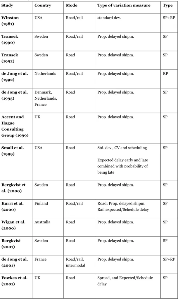
A literature study on how TTV has been measured before has been conducted and is presented in table 1 below. Except identifying the measures used in the studies, any discussions in the studies on which measure to use has also been analyzed. The result is surprisingly meager. Most studies have used a measurement that suits their survey method, without discussing the general pros and cons of different measures.
For the actual measure used for TTV all studies used one of the following four measures, (1) Standard deviation, (2) spread, usually defined as difference between percentiles, (3) percentage of shipments delayed, and (4) average delay (if delayed). Another way to describe the studies is whether or not a scheduling approach has been used. The scheduling utility approach has been used extensively for passenger traffic. The main feature of scheduling is to consider how an actor’s utility for the activity generating a transport changes as a function of time, often delivery and departure time for a freight transport. This is then used to derive an expression for the utility. Typically, all studies in table 1 where scheduling approach has been used, has used the so called α-β-γ preferences, where α is the marginal utility for travel time and β and γ denotes constant marginal utilities for early and late delivery (often called delay early and delay late). Scheduling approach does not restrict the measures used for TTV. All for measures given above may be used in this approach. When scheduling approach is not used VTTV is typically incorporated in the utility of a choice model by adding a term for a suitable TTV measure multiplied by a parameter.
Of the first eleven studies, from 1981 to 2001, eight used proportion of delayed shipments as a variability measure, while one used standard deviation, one study used a both standard deviation and a scheduling approach and one study used proportion of delayed shipments and a scheduling approach. For the last eleven studies, from 2001 to 2012, five studies used proportion of delayed shipments as variability measure, three studies used standard deviation, two studies used scheduling approaches and one study (Henscher et al. 2005) used a combination of different measures. Though proportion of delayed shipments is the most common measure of variability over the whole period covered, there is an increasing use of standard deviation and scheduling utility approaches in later studies.
Table 1 Summary of VTTV studies
Study Country Mode Type of variation measure Type
Winston (1981)
USA Road/rail standard dev. SP+RP
Transek (1990)
Sweden Road/rail Prop. delayed shipm. SP
Transek (1992)
Sweden Road Prop. delayed shipm. SP
de Jong et al. (1992)
Netherlands Road/rail Prop. delayed shipm. RP
de Jong et al. (1995)
Denmark, Netherlands, France
Road Prop. delayed shipm. SP
Accent and Hague Consulting Group (1999)
UK Road Prop. delayed shipm. SP
Small et al. (1999)
USA Road Std. dev., CV and scheduling Expected delay early and late combined with probability of being late
SP
Bergkvist et al. (2000)
Sweden Road Prop. delayed shipm. SP
Kurri et al. (2000)
Finland Road/rail Road: Prop. delayed shipm. Rail:expected/Schedule delay
SP
Wigan et al. (2000)
Australia Road Prop. delayed shipm. SP
Bergkvist (2001)
Sweden Road Prop. delayed shipm. SP
de Jong et al. (2001)
France Road/rail, intermodal
Prop. delayed shipm. SP+RP
Fowkes et al. (2001)
UK Road Spread, and Expected/Schedule delay
Spread: the time within which 98% of the deliveries takes place minus the earliest arrival time
INREGIA (2001)
Sweden Road/rail/air Prop. delayed shipm. SP
RAND Europe (2004) Netherlands Road/rail/ inland waterways, sea/air
Prop. delayed shipm. SP+RP
Hensher et al. (2005)
Australia Road Multi actor framework
(transporter/shipper). No single measure, Probability of on-time arrival (transporter), Slowed-down time (shipper), Waiting time (shipper), Probability of on-time arrival (shipper)
SP
Fowkes (2007)
UK Road/rail Scheduling approach; Spread, early start, late arrival, early and late shifts.
SP
Maggi et al. (2008)
Switzerland Abstract mode Prop. delayed shipm. SP
De Jong et al. (2009) Netherlands Road,/rail/ inland waterways/ sea/air Std. dev.
Conversion of Rand Europe (2004) to reliability ratios RR SP Fries et al. (2010) Switzerland Road/rail/ intermodal
Prop. delayed shipm. SP
Halse et al. (2010)
Norway Road Std. dev. SP
Significance, VU University et al. (2012) Netherlands Road/rail/ inland waterways/ sea/air Std. dev. SP
The discussion on TTV-measurements could be divided in two parts: what to measure and how to measure.
Several authors have distinguished three possible units of analysis (Massiani, 2003):
1. Delivery time: the time between the arrangement between the shipper and haulier regarding the consignment of specific goods and the arrival of the goods at the consignee. 2. Transportation time: includes all logistics between origin and destination (loading,
unloading, etc).
3. Travel time: the duration of the travel from origin to destination.
The terminology has its origin with passenger transport, which makes the name of the units somewhat unusual from a freight transport perspective. However, the original names have been kept here. The broader units of analysis (1 and 2) include all aspects of freight transportation, but may also include issues that are not linked to the value of time (Zhang et al, 2005). Most studies have therefore concentrated on the more limited third measure (Zamparini and Reggiani, 2007). Our review shows that a lot of studies measure even more limited units:
4. Mode time: the duration of travel on a specific mode.
5. Link (or node) time: the duration of travel on a specific link (or node).
The next step is to determine how to measure the effects. Value of Reliability (VoR) is often used instead of VTTV. Based on the literature review, the measures of VoR could be grouped in to variants of:
a) Standard deviation
b) Spread (usually defined as difference between percentiles) c) Percentage of shipments that are delayed
d) Average delay (if delayed)
The most interesting measure is the standard deviation. The benefits of standard deviation are mainly theoretical:
In passenger and freight traffic it is usually considered useful if the value of reliability can be transformed into a reliability ratio, i.e. normed against the value of time (reliability ratio = value of reliability / value of time) The benefits are transferability, VoT (Value of Time) is usually available and one wants to be consistent with these, and adaptation to the CBA (de Jong et al, 2009). VoR for passenger traffic is usually measured by standard deviation, which easily transforms into a reliability ratio.
Standard deviation has nice theoretical benefits when using a scheduling model. A scheduling model means that agents hold preferences for timing of activities and that utility is derived from arrival time (being early or late). Provided the standardized distribution is fixed, the
optimal departure time as well as the optimal expected cost depends linearly on the mean and standard deviation of the distribution of trip durations. Both the optimal departure time and the value of reliability depend in a simple way on the standardized distribution of trip durations and the optimal probability of being late, which in turn is given by the scheduling costs (Fosgerau and Karlström, 2009). Standard deviation suits most CBA-contexts.
One drawback of standard deviation (or variance) is that it is hard to grasp for respondents when doing data collection. Most freight transport that include the value of reliability, have used SP or combined SP/RP surveys. The concepts of variance and standard deviation are considered as too difficult for the respondents (shippers and carriers), hence most studies use the probability of delay or the percentage not on time instead (de Jong et al. 2004). In the SP-studies, the only discussion that could be found about measurements concerns which measure that is most significant. One possible interpretation is that the type of measure to be used is best decided during the actual study, one is that there is a great need for a systematical overview.
A desirable property of a measurement is that it should be translatable to a distribution curve. The distribution curve should then correspond to both the way that respondents value reliability and the way different policy measures effect reliability. Average delay (if delayed) does not correspond to a distribution curve (if it is not combined with a measure of the percentage of shipments that are delayed): policy measures that diminishes small delays gets a negative utility. Standard deviation and spread both includes costs of arriving early, while percentage of delayed shipments does not. What is correct is determined by whether there is a cost of arriving early and whether the modelling of the effects pics up this effect.
Measures used in the logistics industry
The logistics industry uses key performance indicators (KPI) to monitor their operations. These are often easy to understand and easy to collect values that give managers a quick overview of the operations. The KPI are constantly monitored to support operational decision making and management. Common KPIs are customer satisfaction, order fulfilment rate (% of orders delivered complete), quality (number of defects, mean time between failure), inventory levels etc. However, many types of measurements are used and there are no standard measurements used in all industries. Also, the definition of the KPIs varies. For example, one company might measure “delivered” when the shipment is sent, while another company measures “delivered” as when the shipment is at the receiver. However, one of the main purposes of the KPIs are to show trends within the company for internal use and therefore not to be comparable between organisation. Most KPI are thus used within one organisation and rarely throughout an entire supply chain. Thereby they often only measure one part of the transport chain and are rarely compatible with other KPIs used in the chain. The use of KPIs is interesting to study to see if there are any general measurements of delays used in the industry today, which there unfortunately is not. The motive for companies, industries and governments to use measures differ. In accordance with their underlying objectives, but independently of their users, measures can be classified into four groups (Andersson et al, 1989; Byrne and Markham, 1991);
as an important source to establish a holistic view of the system under study and to capture how different parts are connected to each other,
as a source to give feedback in order to initiate new and better ways to conduct and handle the measured system,
as a means to clarify goals and objectives to all participants and personnel which means that the measures have to change and new ones need to be introduced when new objectives are introduced,
and as an indicator of the overall development over time and a source to direct policy actions to areas of importance.
An individual company or multi-companies in co-operation (i.e. supply chains), can easily see the importance of the first three goals, while the latter has traditionally been of interest to governments, policy institutes, agencies etc. But the present trend with companies searching for “best practice” means that development over time also becomes an important aspect for supply chain drivers in their desire to gain competitive advantages.
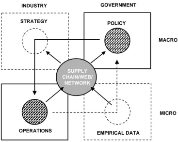
Figure 2 draws on the traditional distinction between industry concern to maximize profit within the constraints given by the governments, and government’s focus on overall sustainability and development of society as an entity involving industry, individuals and relations to surrounding societies. Between these perspectives relations exist as the arrows indicate. In logistics and transportation the pace of the processes shaping the two perspectives is different. With the long investment cycles in physical infrastructure, the governments and society focus on long-term trends and forecasts of future changes. For companies constantly evaluated in the financial market place, all opportunities that in the short run can enhance the competitiveness of a company and its supply chain must be considered.
Figure 2 Schematic description of the logistics evaluation problem in a classic perspective
In Figure 2, these measures are grouped in a macro- and micro-perspective. The arrow from government policy via industry strategy to industry operations is obvious, and has been marked by a solid line, accordingly. If, e.g., there is a new government policy for road transport, this will most certainly affect industry demands and result in modification of strategies. The other arrow from industry operations via empirical data to government policy is marked with a dotted line. This reflects that it is much less difficult for industry to obtain
INDUSTRY GOVERNMENT
MACRO
MICRO
OPERATIONS EMPIRICAL DATA
STRATEGY POLICY
SUPPLY CHAIN/WEB/
data from their operations in a form suitable to support their own strategy modifications than it is for government to obtain empirical data that are suitable for the aggregation necessary to support the formation of new policies.
But the situation for governments is about to change. The fast and unpredictable development of information technology has forced governments to reconsider their long-term goals and focus on shorter perspectives as well. This has led to changes in regulation and the way governments define their role. Today logistics and supply chains to a large extent are built around advances in information and communications. It is inevitable that also in this field societal concerns will shift and as a result will need to address short-term issues in addition to traditional long-term problems.
There are three basic conclusions that can be drawn from this:
The measures currently in use at both macro- and micro-level are inadequate to handle the performance of supply chains and networks making up the national transport structure.
A trend towards highly complex supply webs can be identified which makes it nearly impossible to use “normal” measures since this implies a shift towards other values. There is a need to develop measures on a meso-level, i.e. in between the macro- and
micro-level.
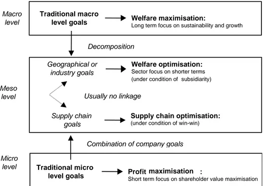
The interaction between the responsibility of industry to create competitive supply chains and the public policy concerns about improving overall efficiency through policy actions requires governmental understanding of the mechanisms affecting the performance of production units, shippers, carriers and other service providers in the supply chain. However, the macro-level focusing on some aspects of welfare maximization can be split into meso-macro-level implying that under subsidiary conditions welfare can be independently maximized for a geographical area or an industry sector. However, as Figure 3 indicates, there is often a linkage between on one hand the macro- and meso-levels and, on the other the supply chain measures aimed to create a win-win situation for the participating companies.
Figure 3 Towards common focus for measures in industry and society
Presently no direct supply chain measures exist. However, our review of other measures currently used in logistics has stressed the importance of suggesting measures, which allow public policy actions to be implemented in a way that supports the desire of industries to develop their competitiveness.
Effects of delays
Freight transport involves a multitude of shipments of different sizes, characteristics and requirements. It involves everything from a 5 000 tonnes slow moving iron ore train to a 100 gram express parcel. The purpose of the shipment could be to deliver a vital spare part that stops the production in an entire factory at huge costs or it could be a load of gravel that just is supposed to be dumped somewhere. This highlights the challenges in determining the effect of delays in the transport chain. The effects of a delay are very contextual. Sometimes a 1 hour late delivery of a single screw can cost millions while in other cases a 1 day late delivery of a shipload of screws can have negligible consequences.
Geographical or industry goals Traditional macro level goals Meso level Welfare maximisation:
Long term focus on sustainability and growth
Macro level
Welfare optimisation: Sector focus on shorter terms (under condition of subsidiarity)
Supply chain goals
Usually no linkage
Supply chain optimisation: (under condition of win-win)
Micro level
Decomposition
Combination of company goals
Traditional micro
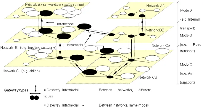
Figure 4 Different modes of transport, networks and gateways (Waidringer, 2001)
Transportation and logistics systems that are the basis for goods transports are quite complex with different modes of transports and interdependencies between buyers, sellers, forwarders etc. The system can be seen as a network of different sub-transport systems connected thorough gateways, which is illustrated in the figure above.
Delays in transport have effect in all parts of the transport network. Direct effects can be seen in longer transport times increasing operational cost of the transport (salary costs, vehicle costs, etc.). Indirect effects can also be seen where the system is affected, not directly by the delay, but by the risk of delays. Transport professionals are well aware of the risk of disruptions in the system and take this into consideration when planning the system. The system thus incurs an indirect cost for backup and flexibility. This can include purchasing more trucks than actually needed to have spare capacity or scheduling an extra train set instead of running a “tight” time table. These effects cannot be allocated to a specific shipment as they are incurred at a system level before the delay has occurred. Further, a disruption also has effects on the transport service quality and thereby on the goods transported and its intended use. For example, production might have to be halted at a receiving factory, overtime cost incurred to catch-up production and customers lost due to failed product deliveries. Table 2 shows common disruption effects in the different parts of the transport system.
Table 2 Activities, link effects, costs and cost drivers for delays
Activity Category Cost Cost driver Key variables Transport Direct
effects
Time dependant vehicle costs
Longer transport time Vehicle costs, length of delay Distance dependent transport cost Longer transport distance
Vehicle costs, extra transport distance
Rescue costs Redirecting other resources to take over planned transport assignments etc.
Cost of extra transport
Indirect effects
Indirect costs for backup and flexibility
Unreliable transport system in general
Perceived reliability, cost of backup
Transport service quality
Goods capital costs Longer transport time Goods value, size of shipment, length of delay
Tranship ment
Direct effects
Staff cost Disrupting terminal operational planning
Staff costs
Terminal storage cost
Missed transhipment Terminal storage costs, size of shipment, length of delay
Transport service quality
Goods capital costs Missed transhipment Goods value, size of shipment, length of delay
Delivery Direct effects
Staff cost Disrupting receiver operational planning Staff costs Use of goods Indirect effects
Cost for safety stock
Unreliable transport system in general
Perceived reliability, cost of safety stock
Transport service quality
Direct cost of lack of goods
Missed customer order etc.
Type of industry, type goods and size of shipment, effects of lacking goods Indirect cost of lack
of goods
Customer choosing other supplier
Type of industry, type goods and size of shipment, effects of lacking goods
Overall chain Direct effects Propagating delays in the chain causing other delay costs
Too small time margins in the transport chain
Characteristics and complexity of transport chain, other cost drivers
Magnitude and frequency of disruptions
The effects of delays caused by the identified factors and drivers are also influenced by the magnitude and frequency of the disruption causing them. A disruption is some unforeseen occurrence in the transport system that causes a delay, for example a traffic accident, extreme weather, congestion, planning mistake etc. The magnitude of the disruption is the size of it, which can be approximated by the length of the delay it causes.
Most disruptions in the freight transport system are of small magnitude, e.g. traffic congestion causing a 20 minute delay. These are frequently occurring but are also expected by the designers of the transport system. Therefore, most transport systems are designed to absorb these small disruptions only with minor consequences, e.g. by planned margins in the time tables or by safety stock. However, the consequences of the disruption increases once the magnitude of the disruption increases past the planned margins. The large magnitude disruptions are less commonly occurring than the small ones which are why they are not planned for in the design of the transport system. The system designers make plans of disruptions that happen once per week but not for disruptions that happens once every decade. The effects of the magnitude and frequency of disturbance are summarised in the figure below, describing the four main types of disruptions and consequences.
Figure 5 The four types of disturbances
It is noteworthy that also arriving too early can cause disruptions. For example, staff might not be available to receive the shipment, a warehouse might be too full to receive more goods, the unloading area might be occupied by other vehicles etc. Often, these early arrivals can be managed by simply waiting, e.g. a truck parks at the roadside and waits until the agreed
M
ag
n
itu
d
e
Large
System killers
Transport
system
with
these
characteristics will be abandoned by
its customer and forced to close.
Catastrophic events
No plans and small
possibilities
to
manage. Very large
consequences.
Contingencies
No plans, but often possible to
manage.
Medium consequences.
Small
Expected risks
Already planned for.
Small consequences.
Common
Rare
is already included in the Expected risks. However, sometimes waiting is not an option, e.g. a train with no available rail siding, or the receiver might choose to receive the shipment anyway. Smaller earlier delivers are already planned for but, similarly to delays when the early delivery goes outside what is planned for in the Expected risks, an extra cost is incurred as in Contingencies. Costs include mainly disrupted operations and possibly extra warehousing and staff costs. Thus, Expected risks and Contingencies do exist also in early deliveries.
How to measure the effects of disruptions
When estimating the effect of disruptions, the System killers can be ignored since they are unlikely to occur over any longer timeframe as a system with such characteristics will be quickly abandoned by its customers. Catastrophic events are truly catastrophic when they occur. These are disruptions such as major natural disasters, major strikes, terrorist attacks etc. Due to their extraordinary and unpredictable characteristics, these are best analyses as special events in a separate risk analysis. These are unstructured scenarios in need for a qualitative evaluation and disaster planning. This is also in line with current principles for passenger transport in the Swedish national planning where “rare events with very large consequences” are recommended to be described qualitatively (Trafikverket, 2012, p. 22). More interesting are the Expected risks and Contingencies. The costs of the Expected risks are already incurred by the design of the transport system. Thus, the delay itself will cause limited extra costs but at the same time, the transports that are not delayed will also have to share the indirect costs for the planned risk, e.g. in safety stock and buffers. However, as soon as the disruption is significant enough to go outside what is planned for, extra direct costs are incurred. The costs of the unplanned disruptions, Contingencies, therefore only impact the transports that are delayed. Planned risks are therefore appropriately measured as shared costs on all transports, while Contingencies are measured as a combination of the shared costs covered by all shipments and added costs from the extra costs from the large disruptions. Similarly, for early deliveries the focus is also in Expected risks and Contingencies. System killers and Catastrophic events can be ignored for early deliveries as it is hard to imagine any disturbance causing very large early deliveries.
Figure 6 General cost structure of transport time variability
The break point between Expected risks and Contingencies (i.e. how long delay that is expected) will vary between different industries and transport chains. The general cost structure of transport time variations can be explained as inFigure 6. The shape of the contingency curve is currently unknown and will require further studies. The contingency costs consist of several factors that are both linear (e.g. salary costs), step wise (e.g. missed onward connections) and non-linear (e.g. disrupted operations). However, it is important that both the costs associated with the Expected risks and the Contingencies are included in the estimation of VTTV.
Several aspects of this categorization need to be further elaborated before applying the model in practice. Time limits between Expected risks, Contingencies and Catastrophic events need to be defined, and as mentioned above, these will vary between industries and transport chains, as some transports are sensitive to disruptions while others have large built-in margins in their system. Furthermore, it is not obvious which exact costs that can be linked to contingencies and expected risks, respectively. These connections need to be rigorously defined in order to present a complete framework for all costs to be included in VTTV.
A method to obtain VTTV
A method has been developed to mathematically estimate VTTV for freight, extending previous studies on VTTV on passenger transport. For passenger transport the scheduling utility approach has been used extensively to obtain VTTV. In a scheduling utility setting a time varying utility is assumed which is associated with activities performed by an individual. The behavior is then derived by maximizing this utility. A common approach is to use a piece-wise linear utility for activities at the destination (Vickrey, 1969; Small 1982; Fosgerau and Karlström, 2010). Often this approach is called α-β-γ preferences, where α is the marginal utility for travel time and β and γ denotes constant marginal utilities for early and late arrival. Some includes an additional discontinuity in the form of a penalty for being late. This approach has been extended by Vickrey (1973) to explicitly include utilities derived from
activities at the origin. A recent application of this is given in Tseng and Verhoef (2008), which in addition replaces the constant marginal utilities with time-varying functions3.
The scheduling approach has been used to obtain VTTV for freight transports (Small et al., 1999; Fowkes et al., 2001; Fowkes 2007). However in both of these freight studies the utility approach from passenger transports has been used. We will reformulate scheduling into using cost functions for the actors involved in freight transports. Assuming the actors are cost-minimizers, similar behaviour as in the utility formulation will be derived. Denoting the conditional, on mode, cost function of a transport by C(m), then the decision problem for the actor is to minimize the cost
minm C(m),
over the given transport modes. If we assume that there are random terms in the cost functions and if we replace the utility with -C(m), then we may estimate VTTV from a discrete choice model as in the studies above. Therefore nothing is lost by switching to a cost formulation of the problem. However, since cost is observable, unlike utility, direct estimation of the cost function, e.g. by a cost-savings method, may be feasible. Hence, formulating the problem in terms of the cost functions of the actors provides more flexibility when estimating VTTV.
There is an essential difference between passenger and freight transport when considering transferring the scheduling utility approach from passenger traffic to freight transports. This is the fact that firms can accommodate increases in transport time variability by planning and taking on cost relate to avoiding disturbances. One such example would be a firm choosing to keep extra safety stock, adding marginal to time tables or investing in spare equipment. Such costs will not be a function of actual transport or delivery times for individual transports; rather these costs will be shared costs for all shipments. The size of the cost, or more precisely how much the company is willing to invest to avoid disturbances, will be a function of the transport time variability σ or more generally, the probability distribution of transport times. We will call these cost abatement costs and denote it as A(σ). This represents the Expected risks in the general cost structure. The running costs, in this context, will be functions of the individual transport or delivery times. Typically, these costs will be operative costs for vehicles and cost associated with loading, unloading as well as transhipping. Since the abatement will determine the running costs, they are also functions of transport time variability. Running costs will be denoted as R(T,D,σ), where T and D are actual transport and delivery times. The running costs are, by definition, functions of actual transport and delivery times. Only the running costs will be involved when transferring scheduling utility approach to freight traffic. Scheduling utility (or in this context, cost) will only cover marginal short run effects with respect to transport time variability when abatement cost may be seen as unchanged and the contribution of transport time variability to the running costs are negligible. In this short run case we simple drop transport time variability from the cost components (marginal costs) in the expressions for running costs. When later extending the cost function with abatement costs transport time variability will also be introduced in all cost components.
3 The authors assume continuity and smoothness of the marginal utilities, this seems to be unnecessary restrictive.
Later when abatement costs is reintroduced in the equations, the resulting VTTV for the total cost has the same form as derived in Andersson et al (2013), which presented VTTV in the following form
(1) VTTV = VTTVL +VTTVλ.
The first term VTTVL represents the marginal change of abatement and running costs when transport time variability change, and the second term represents the changes in the transport time distribution when variability change. Hence the results from a scheduling utility approach and Andersson et al (2013) are basically the same. The earlier result is more general. The main advantage of deriving VTTV from a scheduling approach is that it clarifies the relation between abatement and running costs, that is, between expected risks and contingencies. Further, the result from scheduling is also compatible with several of the methods presented by Krüger and Vierth (2013).
To formulate the problem as a freight delivery situation, assume that there is a preferred delivery time PDT for the goods. To simplify expressions normalize time so PDT is at time zero. Let t denote the departure time from the origin, and D the actual delivery time, then transport time is T = D – t. If we focus on the actor receiving the goods and assume that the marginal costs for travel time, early arrival and late arrival all are constant with values α, β and γ. Then the receiver’s running cost may be written as in (1) which covers the Contingencies in the risk framework developed in the chapter Magnitude and frequency of disruptions above,
(2) R(T, D) = αT + β max(0, −D) + γmax(0, D)
The cost given by (2) has the same form as scheduling utilities with α-β-γ preferences for passenger traffic. Now, with transport time seen as a random variable we will assume that the receiver minimizes the expected cost ER, where R is given by (2). Write transport time as T = μ + σX, where μ is the expected transport time and X is a random variable with EX = 0, representing deviations from the expected transport time. The scale factor σ represents the variability of transport time T. Basically, by applying restrictions on X, σ may be any measure of variability. For example, assumingVar(X) = 1, then σ will be the standard deviation of T. Under these conditions it can be shown (Fosgerau and Karlström, 2010; Fosgerau and Engelson 2011) that the minimum expected running cost is4
(3) ER∗(μ, σ) = αμ + (β + γ)σ ∫1 F−1(s)ds
γ
β+γ ,
where F is the cumulative distribution function (CDF) of X.
The minimum expected running cost in (3) is a function of expected transport time μ and the variability measure σ, but also, through the CDF of X, a function of the probability distribution of transport time. Since information on preferred delivery times may be difficult to obtain, it is an advantage that the entity does not enter the minimum expected cost. Equation (3) provides an immediate expression for the short run VTTV with respect to the variability measure σ, namely
(4) VTTV = (β + γ) ∫1γ F−1(s)ds
β+γ .
To obtain a value for VTTV in a subjective utility formulation of the problem, the marginal utilities α, β and γ needs to be estimated indirectly for example in a choice experiment or an observed discrete choice study. When using the setting of firms as objective cost minimizer’s α, β and γ are interpretable as marginal costs, which may be obtained by studying the receiver’s resource usage as a function of freight delivery time. Typically these marginal costs will be wage rates and capital cost per time unit. Approximate values for these quantities may also be obtained from officially available statistics. The main issue will be to estimate transport time distributions. Also, an appropriate division into shipment classes should be developed e.g. based on the Samgods structure. Should include characteristics such as: type of commodity, size of shipment, transport mode, industry structure etc.
Now, when going from expected short run running costs to expected total costs, equation (4) needs to be modified by adding abatement cost and reintroduce σ into the running cost. This gives us the following expression for the expected total cost, where A(σ) represents the Expected risks and the remaining equation represents the Contingencies :
(5) EC∗(μ, σ) = A(σ) + α(σ)μ + (β(σ) + γ(σ))σ ∫1γ(σ) F−1(s)ds
β(σ)+γ(σ) .
Transport time variability influence the running cost through the marginal costs α, β and γ. In this case equation (5) does not represent the VTTV which isdEC∗⁄dσ. VTTV will contain
two terms, one term describing the change in abatement and marginal costs when σ changes and the other term describing the change in the probability distribution when σ changes. Hence, the form of VTTV will be as given by equation (1) above. To measure VTTV for the total cost, without restricting the scope to short run marginal changes, a study is necessary on how abatement costs and marginal running costs depend on the level of transport time variability. When considering the question of which particular measure to use for travel time variability, the approach behind equation (5) is agnostic. This follows from the arbitrariness of the parametrization of a probability distribution. There is typically an infinite set of different parameters that can be used to describe a particular probability distribution; hence there is an infinite set of equally valid variability measures σ. As discussed above, different measures are obtained by applying different restrictions to the distribution of X.
The steps that is necessary for measuring VTTV by equation (5) is to collect data on the cost components Aσ,ασ, βσ and γσ, and to obtain information of the probability distributions for transport times. Also note that the above equations are for individual shipments. Thus, the method developed does not prohibit using unique values for each shipment, although it is appropriate to group shipments into classes to facilitate data collection. An appropriate division into shipment classes should be developed where groups of shipment are assigned the same values, as e.g. cost of transport are similar for similar shipments. This could be based in characteristics such as: type of commodity, size of shipment, transport mode, industry structure etc.
Conclusions
The original purpose of this project was to identify and evaluate possible measures for quantifying TTV. Literature studies showed that previous studies of the area used different
measures, mostly without discussing which measure to use, and that key performance indicators used in the logistics industry do not fit the purposes of CBA. Furthermore, this study has found that the estimation of the value of TTV – VTTV – can be (and is) derived mathematically independently of which measure that is chosen for the quantification of TTV. In order to actually estimate VTTV in the end – meaning taking all steps including collection of data, statistically analyze it and mathematically derive values – we need to use one or several measures for the travel time variability. However, the mathematical derivation of VTTV proposed above does not put any restrictions on which measure to use.
The valuation of TTV, which is the ultimate aim to which this study contributes, will be based on the cost functions for delays of freight transport. It is the estimation of these functions that will put restrictions on which measure to use, rather than the valuation. It has been concluded that the cost functions will be built up by two parts: 1) fixed abatement cost (costs for expected risks) originating from activities made to handle the general level of transport time variability in the system influenced by the probability distribution of transport times, and 2) delay costs (costs for contingencies) that are functions of the individual delivery times. The more exact shape of this functions need to be estimated by data collection and after that, any restrictions that they put on which measure to use can be described. It is crucial that the chosen measure(s) captures the certain properties of the transport time probability distributions that have impact on both type of costs described above. Therefore, the shape of transport time probability distributions and cost functions need to be further investigated before determining which measure(s) to use for the variability.
Thus, the next step for obtaining VTTV is to collect data on cost functions. In order to be able to use VTTV in CBA, we also need to be able to model the impact on TTV of investments (or other actions) in the infrastructure, i.e. estimate how the transport time probability distributions are affected in different situations (effect relations). The method chosen for doing this, e.g. using Samgods, could put further restrictions on which measure that would be most appropriate to use.
References
Accent and Hague Consulting Group. (1999). The value of travel time on UK roads. Report to DETR, Accent and Hague Consulting Group, London/The Hague.
Bergkvist, E. (2001). Freight Transportation; Valuation of Time and Forecasting of Flows, Umeå Economic Studies, No. 549, Umeå
Bergkvist, E., and L. Westin (2001). Regional valuation of infrastructure and transport attributes for Swedish road freight. The annals of regional science 35(4), 547-560
Andersson, M., Berell, H., Berglund, M., Edwards, H., Flodén, J., Leander, Per., Nelldal, Bo-Lennart., Persson, C.; Waidringer, J. (2013), VTTV FOR FREIGHT TRANSPORT, Report, Swedish Transport Administration, Borlänge, Sweden
Fosgerau, M. and L. Engelson. 2011. The value of travel time variance, Transportation Research Part B: Methodological 45, no. 1, 1-8.
Fosgerau, M. and A. Karlström. (2010). The value of reliability, Transportation Research Part B: Methodological 44, no. 1, 38–49.
Fowkes, A.S., P.E. Firmin, A.E. Whiteling and G. Tweedle (2001): Freight Road User
Valuations of Three Different Aspects of Delay, paper presented and the European
Transport Forum.
Fowkes, T. (2007). The design and interpretation of freight stated preference experiments seeking to elicit behavioural valuations of journey attributes. Transportation Research Part
B: Methodological, 41(9), 966-980.
Fries, N., G. C. de Jong, Z. Patterson, and U. Weidmann (2010). Shipper willingness to pay to increase environmental performance in freight transportation. Transportation Research
Record: Journal of the Transportation Research Board, 2168(1), 33-42.
Halse, A., H. Samstad, M. Killi, S. Flugel and F. Ramjerdi (2010). Valuation of freight transport time and reliability (in Norwegian), TØI report 1083/2010, Oslo
Hensher, D. A., S. M. Puckett, and J.M. Rose (2007). Agency decision making in freight distribution chains: Establishing a parsimonious empirical framework from alternative behavioural structures. Transportation Research Part B: Methodological, 41(9), 924-949. INREGIA (2001): Tidsvärden och transportkvalitet - INREGIA:s studie av tidsvärden och
transport- kvalitet för godstransporter 1999, Underlagsrapport till SAMPLAN 2001:1
de Jong, G.C., M.A. Gommers and J.P.G.N. Klooster (1992): Time valuation in freight
transport: Methods and results, Paper presented at the XXth Summer Annual Meeting,
PTRC, Manchester
de Jong, G. C., Y. van de Vyvere, and H. Inwood (1995). The value of freight transport: A
cross country comparison of outcomes. World Conference on Transport Research, Sydney
de Jong, G.C., C. Vellay and M. Houée (2001). A joint SP/RP model of freight shipments
from the region Nord-Pas-de-Calais. Proceedings of the European Transport Conference
2001, Cambridge.
de Jong, G., E. Kroes, R. Plasmeijer, P. Sanders, and P. Waremius. (2004). The value of
reliability, Proceedings of the European Transport Conference
de Jong, G.C., M. Kouwenhoven, E. P. Kroes, P. Rietveld, and P. Warffemius (2009).
Preliminary monetary values for the reliability of travel times in freight transport. European
Kurri, J., A. Sirkiä and J. Mikola (2000). Value of time in freight transport in Finland. Transportation Research Record: Journal of the Transportation Research
Board, 1725(1), 26-30.
Maggi, R., and R. Rudel (2008). The value of quality attributes in freight transport: Evidence from an SP-experiment in Switzerland. In M. E. Ben-Akiva, H. Meersman, & E. van der Voorde (Eds.), Recent developments in transport modelling, lessons for the freight sector. Bingley, UK: Emerald.
Massiani, J. (2003) Can we use hedonic pricing to estimate freight value of time? Paper presented at the 10th International Conference on Travel Behaviour Research, Lucerne, Switzerland.
RAND Europe (2004). The value of reliability in transport; Provisional values for The
Netherlands. Report TR-240-AVV for AVV, RAND Europe, Leiden, The Netherlands.
Significance, VU University, John Bates Services, TNO, NEA, TNS NIPO and PanelClix (2012). Values of time and reliability in passenger and freight transport in the
Netherlands. Report for the Ministry of Infrastructure and the Environment, Significance,
The Hague.
Small, K. A. (1982). The scheduling of consumer activities: work trips, The American Economic Review 72, no. 3, 467-479.
Small, K., R. Noland, X. Chu and D. Lewis (1999). Valuation of Travel-Time Sav- ings and
Predictability in Congested Conditions for Highway User-Cost Estimation, Report 431,
National Cooperative Highway Research Program, Washington, D.C. Transek (1990): Godskunders värderingar, Banverket Rapport 9 1990:2 Transek (1992): Godskunders transportmedelsval, VV 1992:25
Tseng, Y.-Y. and E. T Verhoef. (2008). Value of time by time of day: A stated-preference
study, Transportation Research Part B: Methodological 42, no. 7, 607-618.
Waidringer, J (2001), Complexity in Transportation and Logistics Systems: An integrated approach to modelling and analysis, Report 52, Dept. of Transportation and Logistics, Chalmers University of Technology, Göteborg, Sweden. Phd Thesis
Vickrey, W. S. 1969. Congestion theory and transport investment, The American Economic Review 59, no. 2, 251-260.
Vickrey, W. S. 1973. Pricing, metering, and efficiently using urban transportation facilities, Highway Research Record 476, HRB, Washington, D.C., 1973, pp. 36-48.
Wigan, M., N. Rockliffe, T. Thoresen and D. Tsolakis (2000). Valueing long-haul and metropolitan freight travel time and reliability. Journal of Transportation and
Statistics, 3(3), 83-89.
Winston, C. (1981). A disaggregate model of the demand for intercity freight transportation.
Econometrica: Journal of the Econometric Society, 981-1006.
Zamparini, L., and A. Reggiani (2007) Freight transport and the value of travel time savings: a meta-analysis of empirical studies. Transport Review, vol 27, No 5 621-636, September 2007.
Zhang, A., A. E. Boardman, D. Gillen, and W. G. Waters II (2005). Towards Estimating the Social and Environmental Costs of Transportation in Canada, A Report for Transport Canada, Vancouver: Center for Transportation Studies.