Does Customer Age Influence Retail Sales? : The Effect of Demographics on Retail Performance

(1)

BACHELOR

THESIS WITHIN:

Economics

NUMBER OF CREDITS:

15

PROGRAMME OF STUDY:

International Economics and Policy

AUTHORS:

Hanna Landegren & Petya Dimitrova

TUTORS:

Sara Johansson & Helena Nilsson

JÖNKÖPING

May 2016

Does Customer Age

influence Retail Sales?

The Effect of Demographics on Retail Performance

(2)

Acknowledgements

We would like to express our gratitude foremost to Sara Johansson and Helena Nilsson for their tutoring, support, and assurance throughout the process of this thesis. Their feedback and guidance throughout this thesis have been invaluable and much appreciated. Additionally, we would like to thank all members of our thesis seminar group for their inputs and contribution.

Finally, we take this opportunity to thank our parents, friends, and loved ones for their support, kindness, and thoughtfulness during every step of the thesis writing process. Each of you have been there to lend a hand throughout our studies abroad at Jönköping University and we are grateful for your unconditional love and encouragement.

(3)

Bachelor’s Thesis within Economics

Title: Younger Customer, Higher Revenue? - The Effect of Demographics on Retail Performance

Authors: Hanna Landegren & Petya Dimitrova Tutors: Sara Johansson & Helena Nilsson Date: 2016-05-23

Abstract

This paper intends to examine whether certain age groups have a positive influence on retail revenue. A large body of work exists on the subject of retailing, however, many fail to show quantitative research on whether demographic characteristics of customers influence retail sales. While previous literature focuses on the supply side of retailing i.e. spatial dependencies between shops, number of competitors, and retail location, the empirical analysis of this paper will rather focus on the demand side of retailing i.e., the customer. A dataset consisting of retail sales, age structures, income, population density and gender ratios of 290 municipalities in Sweden collected in 2014 is used in the empirical testing. The main findings show that age groups between the ages of 18 and 44 have a significant positive influence on retail sales.

Key words: demographics, retail performance, age structure, Central Place Theory, Life-Cycle

(4)

1 INTRODUCTION ... 1

1.1 Delimitations ... 2

1.2 Disposition ... 2

2 PREVIOUS RESEARCH ... 3

2.1 Hypothesis ... 7

3 METHODOLOGY ... 8

3.1 Econometric Model ... 8

3.2 Variables ... 8

3.3 Methodology Shortcomings ... 13

4 RESULTS AND ANALYSIS ... 15

4.1 Regression Analysis ... 15

4.2 Discussion ... 18

5 CONCLUSION ... 20

5.1 Suggestions for Further Studies ... 20

(5)

Figures

Figure 1 Life-Cycle Savings Model ... 4

Figure 2 Central Place Theory ... 5

Tables

Table 1 Variables, Definitions, and Expected Signs ... 10

Table 2 Descriptive Statistics ... 12

Table 3 Highest Retail Sales by Municipality ... 13

Table 4 Initial Regression ... 16

Table 5 Regression with Specifications ... 17

(6)

1 1 INTRODUCTION

This study will focus on the age structures of inhabitants in Swedish municipalities and the respective impact that age has on retail revenue. In this particular case, retail sales growth in Sweden surpasses most other European countries. With high levels of urbanization, large concentrations of wealthy inhabitants, and a liquid retail investment market, Sweden is an attractive area for retailers to locate stores (Lasalle, 2013). As the largest of the Nordic countries, Sweden’s retail sales is expected to grow at a rate of 2.7% in the next three years (Business Sweden, 2013). With high levels of growth in retail, a large number of stores are opening in various regions across the country. Are these decisions influenced by the demographics of the region? Thus, this thesis will explore whether age influences the retail sales in a region.

In general, retailing constitutes a large share of the overall economy in almost all of the countries in the world (Öner, 2014). A large portion of retail literature concentrates on measuring performance through market characteristics such as prices of goods, location of the store etc.; But many ignore the other side of the coin - the customer. By understanding customer values, which can arise from specific demographics, the retailer creates a competitive advantage for itself and its ability to outperform others (Samli, Kelly, & Hunt, 1998). In support of Panigyrakis and Theodoridis (2007), and Terzi, Mutlu, and Dokmeci (2006), this thesis hopes to show how the fast moving and competitive environment within retailing requires a customer focus at all times. The customer has become increasingly important for retailers location strategies and has provided various insights into what role demographics has in shaping these decisions.

Businesses market their products and services through targeted approaches to different segments of the population. Picking the right segment of the market achieves sufficiently large sales volume and profitability for companies. When it comes to the success in retail, the old mantra of “location, location, location” has been replaced by “customer, customer, customer” (Wilson, 2014, p. 124). Even though retailers can have the best locations in terms of visibility and access to other factors, if they do not understand the customer living within close proximity, nothing else matters for the success of the firm. The way to understand the customers’ purchasing behavior is by comprehending their individual characteristics. Therefore, the intent of this thesis is to uncover the extent to which these individual characteristics, specifically age, affect retail performance. In light of this, Crask and Reynolds (1978) find that regular customers of department stores tend to be younger, more educated, and have higher incomes. Additionally, Taylor and Cosenza (2002) find that teens are today’s most influential trailblazer and account for as much as 153 billion U.S. dollars in buying power within the United States. Taking these findings into account, testing whether age of the consumer has a positive influence on retail sales in a region has a clear motivation.

(7)

2

The purpose of this thesis is to gain new insights into the field of retailing and provide new empirical evidence into the influence that demographics may have on retail performance. Many works fail to show quantitative research with observable data on the subject. Therefore, this thesis aims to resolve part of the existing research gap with respect to the effect demography may have on retail performance. Specifically, this thesis aims to explore whether certain age cohorts have stronger influence on retail sales than others. This thesis will use age structure and retail sales data of 290 Swedish municipalities in the year 2014 to test whether certain age cohorts are positively correlated with retail sales. With its innovative market, as mentioned above, and maturity in the retail sector, Sweden is used as the country of research. Thus, the research question in focus is:

How does the demographic profile of regions influence retail performance in Swedish municipalities?

The main findings in this thesis show that the age of customers between 18 and 44 is positively related to the retail sales in a municipality. Such findings indicate that the retail performance in a municipality is shaped by the demography of that region. Furthermore, these results specify the importance of demographics as an influencing factor in retailers marketing strategies.

1.1 Delimitations

Delimitations are applied to this thesis. The availability of specific retail data on the municipal level in Sweden is vast, however, data collected for the regression analysis is limited to one year, as all the data is not accessible to the general public. In addition, the retail data obtained for measuring retail performance is revenue and is aggregated rather than separating each individual sector within retail. These individual sectors include non-durable vs. durable goods, high-order vs. low order goods and the service sector (Klaesson & Öner, 2014). The aggregation of the retails sector despite its heterogeneity is done in order to get a broad overview of how inhabitants’ age influences retail performance since little empirical evidence exists thus far. The correlation and impact age has on retail sales when controlling for additional independent variables will be tested.

The uniqueness of characteristics in Sweden and differences these characteristics may have with other regions, limits the direct ability this research has for enriching retailers strategies in other countries. Nonetheless, since retail theory has been widely studied, and market research has such a wide scope but lacks more empirical evidence, this thesis can be useful for retailers and policy makers in Sweden and possibly on a more global scale.

1.2 Disposition

This paper is organized as follows: Section 2 presents the research and theory behind retailing and previous empirical findings with regards to retail performance. Section 3 states the methodology. Section 4 states the results and analysis and is followed by a conclusion in Section 5.

(8)

3 2 PREVIOUS RESEARCH

The Life-Cycle Savings Model developed by Franco Modigliani is a natural starting point for describing the potential differences in customers shopping behavior. Modigliani developed a practical application of economic theory through the analysis of personal savings in his Life–Cycle Savings Model. Modigliani explains how individuals obtain wealth during younger working years and use this wealth to consume during their lifetime (Ando & Modigliani, 1963).

The income of an individual can be split between savings and spending. When looking into retail performance, the decision of people to save is essential since an increase in savings will lead to a decrease in current purchasing power. People choose to save in order to meet future, long-term objectives. The amount of these savings dependson the different stages of an individual’s life. The Life-Cycle Savings Model is an early example of testing why savings rates vary by age, and in a broader sense, it explains how population age structure influences aggregate savings (Mason, Mayer & Wilkinson, 1993). Moreover, as savings ties directly to expenditures, the level of expenditure also changes with the different stages of life. The early stages of life are associated with substituting current consumption for future. In contrast, the later stages of life correspond to savings, which will be used for repaying the earlier borrowing, and consumption in the years when the individual is retired. The distribution of consumption across the life stages is defined as intertemporal substitution. Without saving or borrowing, the consumption for a given year will be equal to the income of that year, which is not efficient. This is not economical because in certain stages of life, an individual’s income is not high enough to meet his/her needs. The Life-Cycle Savings Model describes how individuals exchange economic resources for goods and services in order to maximize their utility (McDowell, 2012).

Figure 1 represents a simple version of the Life-Cycle Savings Model and shows the individual’s

consumption and savings patterns, as well as the individual’s wealth through life. The figure shows that individuals strive to achieve a constant consumption path throughout their life-cycle. However, this is unrealistic because household consumption will be higher than average when individuals start a family and need to provide for their children (Ando & Modigliani, 1963). One can still use the Life-Cycle Savings Model based on the intuition that consumers in their early adulthood will have large expenditures, such as buying a house and supporting their children. While this model emphasizes the consumer, one can relate the theory to customer behavior. An individual may strive to maintain a normal consumption pattern throughout his/her life, but this does not indicate that each individual buys the same amount of goods and services throughout life stages. Young children many consume close to the same amount of goods as parents would, but they purchase much less because of lack of income. This would support different age groups having different shopping behaviors and hence the possibility that certain age groups could have a larger impact on retail sales than other cohorts.

(9)

4 Figure 1 Life-Cycle Savings Model

The demand and purchase of products are not only dependent on their functions, but also the satisfaction and meaning they create for their owners (Levy, 1963; Tauber, 1972). The Theory of Leisure Class developed by Veblen (1973) shows the importance of the properties an individual owns. Veblen brings the concept of conspicuous consumption and argues that an individual’s social position is associated with the possessions he/she has. This theory is criticized because the dynamics of people’s social life cannot be explained by such a simplified approach (Öner, 2014). Moreover, Pine and Gilmore (1999) show the changes in peoples’ behavior,and that today, the value of the product comes from the experience of consuming a product rather than the actual value of the commodity. Despite this criticism, the Theory of Leisure class pioneered the way we look at social structures and everyday behaviors (Veblen, 1973), and such behaviors are influenced by the age of the individual.

While the Life-Cycle Savings Model puts stress on how much a customer will spend when they shop, and the Theory of Leisure Class describes the satisfaction a customer obtains from goods and services, the Central Place Theory focuses on where a customer will shop. The geographical distribution of the retailing sector is heavily influenced by the density of markets and the location decisions of retailing firms can be described by the Central Place Theory.

The Central Place Theory developed by Christaller and Lösch is pivotal for understanding the spatial organization of retailers and the distribution of goods and services. The "central place" in their analysis is defined as the relationship between individuals and the stores which provide goods and services.

Demand for goods and services is highly determined by distance, and for shoppers located far away from

the center of the market, the demand for these goods will be driven to zero. The benefits and utility gained from shopping in this distant market will not cover the cost required to purchase such goods. The

increase in distance and transportation costs, lead to decreases in demand, which causes smaller

(10)

5

The supply of goods over different locations is deeply discussed in the Central Place Theory. Internal

returns to scale determines this supply. The theory presents a hierarchical system of locations with the

implication that larger cities will have more concentrated activities and present more functions than those covered by smaller cities. This leads to relatively higher revenue in the larger, more populous cities, than insmaller locations. (Lösch, 1954)

A visual representation of Central Place Theory is captured in Figure 2. The figure clearly shows that there is one central location called a ‘city’. The figure also shows how the locations are distributed around this central place and are of various sizes. Figure 2, shows that two large cities are never located directly next to each other. Rather, this even distribution across space allows for smaller towns and villages to locate next to larger cities and have access to a greater variety of goods. Generally, people’s love of variety is captured in more populated areas where individuals work and the growth of these cities can be explained by the endogeneity between consumers and firms.

Figure 2 Central Place Theory

The theoretical models discussed above are used as a guideline when analyzing and interpreting the results obtained. Past empirical work supports these theories and gives knowledge and explanations for the choice of variables in this thesis.

The Central Place Theory discusses the connection between individuals in relation to distance and choice of stores. Proudfoot (1937) explains how the central business district attracts many consumers from outlying areas, and as a result, creates an agglomerate economy. These agglomeration activities are presented by Öner (2014) showing how shops and consumer services are highly related to the economic performance of cities. Further support of these findings is presented by Reilly’s law, which uses a gravitational approach to show how the individual decides which shopping location to favor, and measures the trade between cities as proportional to the population of the cities and inversely proportional to the distance between those cities (Klaesson & Öner, 2014; Ghosh & McLafferty, 1987). Empirical work also shows the importance of distance regarding people’s decision where to shop (Zeithaml, 1988; Öner, 2014; Anderson, Goeree & Romer, 1997). Studies show that people are willing to travel farther in order to buy the goods demanded (O’Kelly, 1981, 1983; Thill & Thomas, 1987). What

(11)

6

it implies is that when people travel to higher-level location shops, such as big cities and towns, as specified by the Central Place Theory, they tend to also buy lower-order goods along with high-order ones. Öner (2014) argues that higher levels of market potential motivate location decisions of retailers. Moreover, Craig, Ghosh and McLafferty (1984), and Ferber (1958) show in their research that retail sales are influenced by the population density variable.

The empirical work connected to the Life-Cycle Savings Model gives additional insights into the shopping behaviors of customers. In addition to the aforementioned, an individual's shopping decisions can be influenced by the prices of goods, which is also reflected by the individual’s income. Russell (1957) found a positive correlation between income and retail sales adjusted for population. The wealth of an individual determines the choice of where he/she will shop. Moreover, it could be assumed that higher-level locations provide lower prices due to increased supply and competition. These factors make the larger locations more attractive for the customers, and the location of retail is determined by the size of market potential (Klaesson & Öner, 2014; Terzi et al., 2006). Bliss (1988) supports this by the finding that a very poor individual is willing to travel larger distances in order to minimize the purchasing costs.

Furthermore, empirical tests from Miller and Kean (1997) show that there is a positive relationship between consumer’s objective to shop locally and numerous demographic variables. In order to know where on the life-cycle a consumer may be the age of children is used in the analysis (Miller & Kean, 1997). Not to mention, support is given by Lee (2003), who shows that younger individuals are consuming and spending more than they are producing, and the opposite is observed in the case of adults.

The Theory of Leisure Class goes one step further in the analysis of people’s shopping behavior. The empirical work connected to this theory shows that customers of different age and gender obtain different levels of satisfaction, or utility, from the same product (Moschis, 1992). The contentment of owning a product can depend on the age of the customer. Mason et al. (1993) observe shoppers around and above 30 years old to be more diversified and have higher expectations in their choice, in terms of size, shapes and tastes, than younger people. Additionally, the gender of an individual plays an important role in the empirical findings (Taylor & Cosenza, 2002; Siu & Tak-Hing Cheung, 2001). Hanson and Hanson (1980) support the outcome that women shop more frequently than men.

What more determines individual’s preferences is the surrounding environment. Uhrich and Tombs (2014), suggest the effect others have on individual's self-awareness, and that individuals can ease other shoppers' evaluative concerns. Tauber (1972), analyzes the effect peer groups have on peoples’ decisions. Underpinning the theory of Leisure Class, people have the tendency to buy the same products as the members of a group that they desire to belong to. Tauber (1972) argues that record stores are a common place for teenagers to spend their spare time, which leads to an increase in the shops performance at this place because peers tend to have the same shopping preferences.

(12)

7

Despite the statements from previous literature, some researchers argue that demographics may not be a relevant factor in representing customer behavior. Mason and Burns (1999), state that customers may have very similar profiles, but have large differences in taste, interest and choices. This thesis works against these claims, and strives to find a relationship between retail performance and age of the shopper based on facts and empirical testing.

2.1 Hypothesis

The concepts underlining Central Place Theory, Life-Cycle Savings Model, Leisure Class Theory, and the empirical works presented earlier provide different examples of what contributes to retail performance. Some theories suggest different demographic and/or spatial/market variables to play a predominant role in determining the potential for retail sales in a municipality. According to Central Place Theory, variables such as population density of municipalities in relation to the overall amount of agglomeration in the economy could have the biggest impact on retail performance in a region. In support of this claim, data shows that larger municipal areas such as Stockholm, Malmö, and Gothenburg have very high levels of retail revenue in contrast to smaller towns in the North of Sweden.

According to theory and previous studies, there are a multitude of variables that could impact the retail sales of a region. These include: age, gender, income, population, and supply side variables (Tauber, 1972; Miller & Kean, 1997; Taylor & Consenza, 2012). Considering the lack of empirical testing and statistical evidence on the topic, this thesis will test the relationship between various age cohorts in each municipality in Sweden and the corresponding retail sales these groups generate. Based on previous literature, we expect that large shares of young adults will positively influence retail sales in municipalities. The tested hypothesis in the thesis is:

(13)

8 3 METHODOLOGY

To obtain results, cross-regional data is used in the analysis to give a representation of the relationship among the variables. The empirical data for this thesis is based on 290 observations at the Swedish municipal level in the year 2014, and is found at SCB (Statistics Sweden) and HUI (Swedish Institute of

Retail), with consideration to the limitations these sites may possess, i.e. lack of available data. The

quality of the data collected is assured by obtaining measurements from well-developed research and statistical institutions.

3.1 Econometric Model

This thesis is interested in uncovering the relationship between customer age and its’ effects on retail performance, and determining the overall statistical significance of the variables. Based on the theoretical framework and empirical work in previous research, the following econometric model is formulated for the analysis:

Equation 1

𝐿𝐿𝐿𝐿(𝑅𝑅𝑅𝑅𝑣𝑣𝑅𝑅𝐿𝐿𝑒𝑒𝑅𝑅𝑖𝑖) = 𝛽𝛽0+ 𝛽𝛽1𝐿𝐿𝐿𝐿�𝑃𝑃𝑃𝑃𝑃𝑃𝑑𝑑_𝑖𝑖� + 𝛽𝛽2𝐿𝐿𝐿𝐿(𝐼𝐼𝑖𝑖) + 𝛽𝛽3(𝐺𝐺𝑖𝑖) + 𝛽𝛽4(𝑆𝑆𝐷𝐷𝑖𝑖) + 𝛽𝛽5(𝐴𝐴𝐴𝐴𝑅𝑅𝑖𝑖) + 𝜀𝜀𝑖𝑖

The equation above represents the relationship between retail performance and a set of given explanatory variables. The explanatory variables in this regression include an intercept term (𝛽𝛽0), the population density (𝑃𝑃𝑃𝑃𝑃𝑃𝑑𝑑), gender ratio (𝐺𝐺), income (𝐼𝐼), the spatial dependency variable (SD), shares of various age groups (𝐴𝐴𝐴𝐴𝑅𝑅), and an error term (𝜀𝜀𝑖𝑖) which is expected to follow a normal distribution.

3.2 Variables

Dependent Variable

Retail revenue as the financial indicator of the firm’s performance will be used as the dependent variable in this thesis. It aims to test the determinants of such retail sales. Retail revenue is expressed as the total sales (in thousand SEK) in the aggregated retail sector for each Swedish municipality in 2014 and is logged in the analysis. The data shows that the variable varies greatly between municipalities. The year 2014 is chosen because it captures some of the most recent data as far as consumption patterns in the retail industry in Sweden. Furthermore, it is the most recent year with accessible data on the HUI statistical database.

(14)

9

Independent Variables

The independent variables consist of both spatial/market variables and demographic variables. These spatial/market variables include measurements for the overall economic performance. Demographic variables are representative characteristics of the population in Sweden comprised of 290 municipalities, which are defined as the smallest regional divisions with their own administration. The aforementioned empirical works are used as a base for the choice of variables in this thesis. The age variable as the variable of interest in this thesis is supported by works of Miller and Kean (1997), Taylor and Consenza (2002), and the Life-Cycle Savings Model. Age presented in the analysis is broken down into the following cohorts: 0-17, 18-24, 25-44, 45-64, and 65+. The age groups presented in Table 1 are chosen as the target groups in this thesis because each variable represents the different stages in one’s life. Individuals often live at home between the ages of 0-17, begin university studies between 18 and 24, start a family from 25-44, support family and prepare for retirement during the ages of 45-64, and retire after the age of 65. Additional variables included in the analysis of past literature are: income, gender ratio and population density (Ferber, 1958; Lee, 2003; Terzi et al., 2006; Uhrich & Tombs, 2014). Ferber (1958) concluded a support for Reilly’s Law of Retail Gravitation in that both population (and population density), and distance influence changes in retail sales between cities. In support of Öner (2014), the authors use gender ratio as an explanatory variable for explaining retail revenue. Additionally, the theory of Leisure Class gives insights into including gender ratio in the regression analysis. This variable controls for the effects of customer age on retail performance since it may skew the results if not taken into account. If the gender ratio is large enough, this could have impacts on retail revenue within certain sectors.

A spatial dependency variable is included in this thesis to alleviate possible autocorrelation that may occur during the regression analysis. In cross-regional data, spatial autocorrelation may arise between locations. Testing the total retail revenue in 290 municipalities in Sweden is likely to create such spatial dependencies. According to the Central Place Theory, the larger cities may minimize the ability for stores to open up in smaller areas surrounding the city, as most of the population drives to the central location to buy goods, despite transportation costs they incur. Anselin (1988) describes spatial econometrics as the collection of techniques that deal with the peculiarities caused by space. The importance of spatial interaction is crucial in economic testing, and for this thesis, which analyzes the spending pattern across municipalities in Sweden. The spatial dependency variable is designed as follows:

Equation 2

𝑆𝑆𝐷𝐷 = 𝐿𝐿𝐿𝐿(∑ 𝑅𝑅𝑅𝑅𝑅𝑅𝑅𝑅𝑅𝑅𝑅𝑅 𝑆𝑆𝑅𝑅𝑅𝑅𝑅𝑅𝑆𝑆 𝑅𝑅𝐿𝐿 𝐹𝐹𝐴𝐴𝑛𝑛− 𝑅𝑅𝑅𝑅𝑅𝑅𝑅𝑅𝑅𝑅𝑅𝑅 𝑆𝑆𝑅𝑅𝑅𝑅𝑅𝑅𝑆𝑆 𝑅𝑅𝐿𝐿 𝑀𝑀𝑒𝑒𝐿𝐿𝑅𝑅𝑀𝑀𝑃𝑃𝑅𝑅𝑅𝑅𝑅𝑅𝑅𝑅𝑦𝑦_𝑁𝑁 𝑛𝑛)

Where SD measures the spatial dependency variable, ∑ 𝑅𝑅𝑅𝑅𝑅𝑅𝑅𝑅𝑅𝑅𝑅𝑅 𝑆𝑆𝑅𝑅𝑅𝑅𝑅𝑅𝑆𝑆 𝑅𝑅𝐿𝐿 𝐹𝐹𝐴𝐴𝑛𝑛 measures the sum of the total retail sales in a given FA region, 𝑅𝑅𝑅𝑅𝑅𝑅𝑅𝑅𝑅𝑅𝑅𝑅 𝑆𝑆𝑅𝑅𝑅𝑅𝑅𝑅𝑆𝑆 𝑅𝑅𝐿𝐿 𝑀𝑀𝑒𝑒𝐿𝐿𝑅𝑅𝑀𝑀𝑃𝑃𝑅𝑅𝑅𝑅𝑅𝑅𝑅𝑅𝑦𝑦𝑛𝑛 is the total retail sales in a

(15)

10

municipality in the given FA region, and N is the number of municipalities in a given FA region. FA regions are functional analysis regions that comprise a total of 72 in Sweden in 2005 (SCB).

Based on aforementioned research and empirical works of the effects on retail performance, the econometric model of this thesis presents the following independent variables and their expected signs in the table below:

Table 1

Variables, Definitions, and Expected Signs

Variable Definition Expected sign

Population Density (𝑷𝑷𝑷𝑷𝑷𝑷𝒅𝒅)

Log of total number of persons per sq. km in each municipality

+

Income (𝑰𝑰)

Logged mean net income per individual in each

municipality

+

Gender Ratio (𝑮𝑮)

Proportion of women to men in each municipality

+

Spatial Dependency (𝑺𝑺𝑺𝑺)

Log of the retail sales in a municipality compared to the average sales in the FA region

n/a

Age Structure (𝑨𝑨𝑨𝑨𝑨𝑨)

Share of different age groups in municipalities total population

(𝑨𝑨𝑨𝑨𝑨𝑨𝟎𝟎_{𝟏𝟏𝟏𝟏}) Fraction of municipalities _{total population 0-17} -

(𝑨𝑨𝑨𝑨𝑨𝑨𝟏𝟏𝟏𝟏_{𝟐𝟐𝟐𝟐}) Fraction of municipalities _{total population 18-24} +

(𝑨𝑨𝑨𝑨𝑨𝑨𝟐𝟐𝟐𝟐_{𝟐𝟐𝟐𝟐}) Fraction of municipalities _{total population 25-44} +

(𝑨𝑨𝑨𝑨𝑨𝑨𝟐𝟐𝟐𝟐𝟔𝟔𝟐𝟐) Fraction of municipalities total population 45-64 +/- (𝑨𝑨𝑨𝑨𝑨𝑨𝟔𝟔𝟐𝟐+) Fraction of municipalities total population 65+ +/-

(16)

11

Table 1 shows that age structures 18-24 and 25-44 are expected to have a positive influence on retail

performance. Individuals between 18 and 24 are expected to be students and spend all of their income on their own needs and desires. Individuals between 25 and 44 are expected to be in a stage of their lives when it is common to start a family and their consumption power increases from employment. The other age groups are expected to have unpredicted and/or negative signs. The age group below 18 years old is expected to earn little or no income and parents are expected to support their needs financially. In addition, the age group 45-64 has an unpredicted sign as this age cohort is expected to start saving more in preparation for retirement but may still have large expenditures for their children as shown in the Life-Cycle Savings Model. The oldest age group containing individuals above the age of 65 is expected to have an unpredicted sign. The unpredicted sign can be explained by the fact that 65 year old and older are expected to be in retirement and may economize more, however, the older generation in today’s world is much different than it was 50 years ago. Therefore, this age group could have higher incomes and purchasing power than older generations before them, and in turn, be positively correlated with retail sales.

The gender ratio variable is expected to have a positive sign based on the research of Taylor and Cosenza (2002),and Hanson and Hanson (1980) as it represented the ratio of the total number of women to the total number of men. Income is expected to have a positive relationship with retail revenue based on the intuition that individuals with higher incomes will purchase more goods due to a larger disposable income. Population density is also expected to have a positive influence on retail sales because larger populations lead to greater amounts of economic activity in a location. The spatial dependency variable has no expected sign as it is designed to take away from potential autocorrelation in the model.

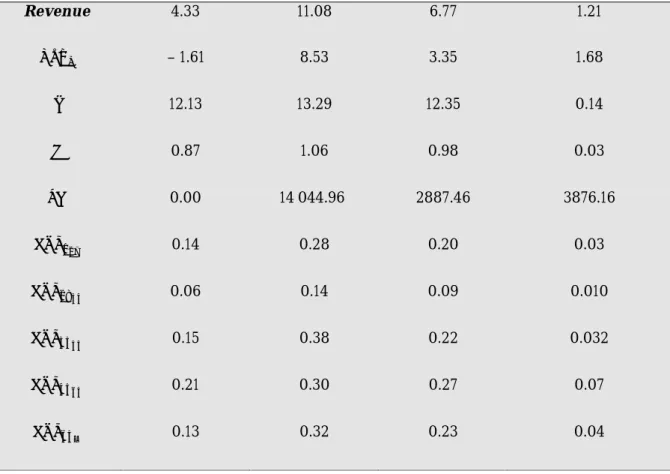
In Table 2, the descriptive statistics are presented to give an initial summary of the age variables. Table

2 shows the minimum, maximum, mean, and standard deviation of each variable used in the regression

analysis. The revenue, population density, and income are logged in this model. The mean value of each age group provides indications of the general age composition within each municipality in Sweden. The table shows that individuals between 45 and 64 make up the largest population in Sweden. In addition the gender ratio varies throughout certain municipalities which may influence the results, but generally, the mean shows that the ratio between men and women is quite even. The mean of age group 18-24 shows the smallest percentage of population in Sweden, and is to be expected as this age cohort only includes individuals within a 6 year time span.

(17)

12 Table 2

Descriptive Statistics

Variable Minimum Maximum Mean St.d. Deviation

Revenue 4.33 11.08 6.77 1.21 𝑷𝑷𝑷𝑷𝑷𝑷𝒅𝒅 – 1.61 8.53 3.35 1.68 𝑰𝑰 12.13 13.29 12.35 0.14 𝑮𝑮 0.87 1.06 0.98 0.03 𝑺𝑺𝑺𝑺 0.00 14 044.96 2887.46 3876.16 𝑨𝑨𝑨𝑨𝑨𝑨𝟎𝟎𝟏𝟏𝟏𝟏 0.14 0.28 0.20 0.03 𝑨𝑨𝑨𝑨𝑨𝑨𝟏𝟏𝟏𝟏_{𝟐𝟐𝟐𝟐} 0.06 0.14 0.09 0.010 𝑨𝑨𝑨𝑨𝑨𝑨𝟐𝟐𝟐𝟐_{𝟐𝟐𝟐𝟐} 0.15 0.38 0.22 0.032 𝑨𝑨𝑨𝑨𝑨𝑨𝟐𝟐𝟐𝟐_{𝟔𝟔𝟐𝟐} 0.21 0.30 0.27 0.07 𝑨𝑨𝑨𝑨𝑨𝑨𝟔𝟔𝟐𝟐₊ 0.13 0.32 0.23 0.04

Table 3 presents the 10 municipalities with the highest retail sales in Sweden and the corresponding

shares of each age group within that municipality. As can be seen in the table below, the municipalities with the largest retail sales are some of the most densely populous regions in Sweden, respectively. It would be expected that the three metropoles in Sweden (Stockholm, Gothenburg, and Malmö) have the highest retail sales due to the high agglomeration of retail in these locations. In addition, some of the largest universities in Sweden are located in these cities providing evidence that a high share of younger individuals could reside in these areas. This could support the hypothesis that larger shares of young adults positively influence retail sales. In addition, Table 3 indicates that the 10 municipalities with highest retail sales also have some of the highest shares of individuals between 25 and 44 in Sweden. This may indicate a positive relationship between this age group and retail sales and will be tested further in the regressions in the next chapter.

(18)

13 Table 3

Highest Retail Sales by Municipality

Municipality 𝑨𝑨𝑨𝑨𝑨𝑨𝟎𝟎𝟏𝟏𝟏𝟏 𝑨𝑨𝑨𝑨𝑨𝑨𝟏𝟏𝟏𝟏𝟐𝟐𝟐𝟐 𝑨𝑨𝑨𝑨𝑨𝑨𝟐𝟐𝟐𝟐𝟐𝟐𝟐𝟐 𝑨𝑨𝑨𝑨𝑨𝑨𝟐𝟐𝟐𝟐𝟔𝟔𝟐𝟐 𝑨𝑨𝑨𝑨𝑨𝑨𝟔𝟔𝟐𝟐+ Revenue (000’s) 𝑷𝑷𝑷𝑷𝑷𝑷𝒅𝒅 Stockholm 0.20 0.08 0.34 0.23 0.14 64898 4872.80 Göteborg 0.19 0.10 0.32 0.23 0.15 38850 1208.20 Malmö 0.20 0.09 0.33 0.22 0.15 22805 2031.30 Uppsala 0.20 0.12 0.29 0.23 0.16 14147 95.00 Västerås 0.20 0.10 0.26 0.25 0.20 11570 149,90 Huddinge 0.25 0.09 0.29 0.24 0.13 11452 795.10 Örebro 0.21 0.11 0.27 0.23 0.18 11027 103.90 Linköping 0.20 0.12 0.28 0.23 0.17 10933 106.40 Helsingborg 0.20 0.09 0.26 0.25 0.19 10437 393.60 Jönköping 0.21 0.11 0.26 0.23 0.19 9569 89.30

3.3 Methodology Shortcomings

Various diagnostics tests are run to test for the validity of the model and the authenticity of the variables used in this thesis. Initially, a correlation matrix is used to interpret the interconnection between a series of variables in the data set. The correlation matrix computes the correlation coefficient between variables and uses the two tailed Pearson correlation test to analyze the significance among the variables. Data showing a significance level that is lower than 0.05 shows coefficients that are highly statistically significant. The correlation matrix presented in the Appendix shows that the age groups are both positively and negatively correlated to each other. This is expected as the age groups are measured in shares. The correlation matrix also shows that some correlation exists between income and age. Despite this, income levels should be included in the regression analysis because it will be certain that by including income in the model, the effect of age on retail revenue will not be an income effect but an age effect. The presence of correlation between the explanatory variables could create a problem of multicollinearity. Multicollinearity is the presence of correlation amongst the variables and could be an

(19)

14

explanation of insignificant coefficients. This thesis looks at the variance inflation factors (VIF) in order to test for multicollinearity. Some variables have a VIF higher than 10 which indicates a presence of multicollinearity. Remedies for multicollinearity consist of doing nothing, omitting redundant variables, increasing the sample size, or transforming variables. In support of previous research, income, population density and gender ratio are the desired control variables and are therefore analyzed in this thesis despite the presence of multicollinearity because without these variables, an omitted variable bias would be created. In addition, a second regression is run where five specifications for age are used when testing for significant effects on retail revenue to take away from the multicollinearity shortcoming between the age groups.

The consistency and stability of the chosen regression model is analyzed by using the Shapiro-Wilk test for normality. The values obtained in the Shapiro-Wilk’s test are higher than 0.05 which is an indicator for normality in our model. Heteroscedasticity is tested for using the Breach-Pagan and White tests and conclude the diagnostic tests for this thesis. Heteroscedasticity occurs when the error terms in the regression have no constant variance and when the error terms are dependent on some explanatory variable (Gujarati, 2009). The Breach-Pagan and White tests present values at the 0.05 level indicating a presence of heteroscedasticity (see Appendix). In order to deal with this shortcoming, robust standard errors are used to analyze the accurate significance of the tested variables. In addition, the shortcoming that spatial dependency creates among variables tested is alleviated through the use of a spatial dependency variable in the model.

One shortcoming other than the multicollinearity and heteroscedasticity of the model, is the endogeneity within the model design. One can have different hypotheses on the causality of certain variables. In order to test the causality between variables, time series data is needed. However, this thesis cannot test the causality between retail revenue and the explanatory variables as the data is limited to 1 year. Despite this shortcoming, conclusions and inferences from the theory presented earlier can still be made. Empirical works show that the location of retail services is concentrated to places with large levels of market potential and areas where demand is high (Öner, 2014; Hernant, 2009; Ziethaml, 1988). This research supports the argument that the retailer attracts the customer, which in turn improves sales. For further support, one can turn to Table 3, which shows a possibly high correlation between different age groups agglomerating in populous cities and high levels of retail sales. It is challenging to make claims on the influence certain variables have on other variable. However, if the model designed in this thesis could show that young adults do indeed purchase more in retail than other age cohorts, we could support the possibility that the demographics in a region attract strong shopping nodes.

(20)

15 4 RESULTS AND ANALYSIS

The following chapter will present the results of various regressions and analyze the statistical significance of these results. A complete analysis of the presented model, descriptive statistics, and regression results will be provided. A discussion of the empirical findings will conclude this section.

4.1 Regression Analysis

The regression analysis of this thesis uses the natural logarithm of certain independent and dependent variables in the data set to enhance the fit of the model. When residuals are not normally distributed, the logarithm of the variable may improve this fit. Calculating the logarithm of the variable will change the scale of the variable. Furthermore, the estimated coefficients of the logged regressand and regressors show elasticities when the log of each variable is calculated. On the one hand, a logged regression can be interpreted as:

𝐴𝐴 1% 𝑅𝑅𝐿𝐿𝑀𝑀𝑖𝑖𝑅𝑅𝑅𝑅𝑆𝑆𝑅𝑅 𝑅𝑅𝐿𝐿 𝑋𝑋 𝑤𝑤𝑃𝑃𝑒𝑒𝑅𝑅𝑤𝑤 𝑅𝑅𝑅𝑅𝑅𝑅𝑤𝑤 𝑅𝑅𝑃𝑃 𝑅𝑅 𝛽𝛽% 𝑅𝑅𝐿𝐿𝑀𝑀𝑖𝑖𝑅𝑅𝑅𝑅𝑆𝑆𝑅𝑅 𝑅𝑅𝐿𝐿 𝑌𝑌 𝑀𝑀𝑅𝑅𝑅𝑅𝑅𝑅𝑖𝑖𝑅𝑅𝑆𝑆 𝑃𝑃𝑅𝑅𝑖𝑖𝑅𝑅𝑝𝑝𝑒𝑒𝑆𝑆

On the other hand, the interpretation of a log-lin model in the case of the explained retail revenue variable and explanatory age structure variables in this thesis is given by the following (Gujarati, 2009):

𝐼𝐼𝐼𝐼 𝑋𝑋 𝑅𝑅𝐿𝐿𝑀𝑀𝑖𝑖𝑅𝑅𝑅𝑅𝑆𝑆𝑅𝑅𝑆𝑆 𝑝𝑝𝑦𝑦 𝑃𝑃𝐿𝐿𝑅𝑅 𝑒𝑒𝐿𝐿𝑅𝑅𝑅𝑅 𝑌𝑌 𝑅𝑅𝐿𝐿𝑀𝑀𝑖𝑖𝑅𝑅𝑅𝑅𝑆𝑆𝑅𝑅𝑆𝑆 𝑝𝑝𝑦𝑦 �𝑅𝑅𝛽𝛽𝑖𝑖− 1� ∗ 100%

The model of this thesis uses a mix of logged and unlogged variables. The logged variables include: revenue, population density, and income. The variables that are not logged in this thesis include: gender ratio, and the spatial dependency variable. The variable of interest, age, is also not logged as the variable is measured in shares of the population. Although the results concerning the variables that are not logged may be harder to interpret theoretically, the regression provides compelling results on which age structures may have the largest impacts on retail revenue.

As a starting point for the regression analysis of this thesis, all variables are included in the empirical model. The regression incorporates all of the age structures defined in this thesis. This initial regression is run to test whether age has any statistical significance for retail revenue despite the correlation that exists among the age group cohorts. The model is presented in Table 4 below and gives a general overview on how the explanatory variables effect the retail sales in a given municipality. Reasons for the delimitation or changes of variables will be described later on.

(21)

16 Table 4

Initial Regression

According to Table 4, income, gender ratio and age groups 0-17, 18-24 and 65+ are significant at the 5% level of significance. Population density, age groups 25-44 and 45-64 are not significant at the 5% level of significance. The goodness of fit between age parameter and the retail performance parameter is analyzed by checking the measure for R-squared. The estimated R square of the model is 0.665, which shows that 66.5% of the change in total revenue is explained by the regressors. Additionally, the measured value of the adjusted R square is equal to 0.654 (see Appendix). The minimal variation between these two values shows support for the choice of the independent variables in the OLS regression analysis. The R of the model also suggest for the existence of latent variables. Since the shopping behavior of an individual is not measurable, the analysis of this paper is on the age of the customer and the control variables income and gender ratio.

Variables 𝜷𝜷 t Constant -13.765 -1.559 𝑷𝑷𝑷𝑷𝑷𝑷𝒅𝒅 0.016 0.358 𝑰𝑰 1.183** 2.437 𝑮𝑮 13.403*** 7.058 𝑺𝑺𝑺𝑺 -1.217E-006 -0.111 𝑨𝑨𝑨𝑨𝑨𝑨𝟎𝟎𝟏𝟏𝟏𝟏 -24.309*** -3.622 𝑨𝑨𝑨𝑨𝑨𝑨𝟏𝟏𝟏𝟏_{𝟐𝟐𝟐𝟐} 19.354** 2.421 𝑨𝑨𝑨𝑨𝑨𝑨𝟐𝟐𝟐𝟐_{𝟐𝟐𝟐𝟐} 5.452 0.792 𝑨𝑨𝑨𝑨𝑨𝑨𝟐𝟐𝟐𝟐𝟔𝟔𝟐𝟐 -7.942 -1.062 𝑨𝑨𝑨𝑨𝑨𝑨𝟔𝟔𝟐𝟐+ -13.800** -2.062 R 0.816 R-Squared 0.665 Observations 290

Dependent Variable: Revenue ** Significant at 0.05 level *** Significant at 0.01 level

(22)

17

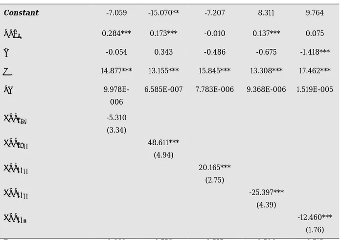
Table 5 demonstrates the regression results obtained for each specific age group independently to

alleviate the insignificance that multicollinearity could have created in the initial regression model (Table 4). This second step in the regression analysis reduces the high collinearity among the age variables that may have mislead the interpretation of the outcome of the coefficients’ significance. Furthermore, it will alleviate the chance that the multicollinearity in the initial model caused the variables to switch signs.

Table 5

Regression with Specifications

Variables 1 2 3 4 5 Constant -7.059 -15.070** -7.207 8.311 9.764 𝑷𝑷𝑷𝑷𝑷𝑷𝒅𝒅 0.284*** 0.173*** -0.010 0.137*** 0.075 𝑰𝑰 -0.054 0.343 -0.486 -0.675 -1.418*** 𝑮𝑮 14.877*** 13.155*** 15.845*** 13.308*** 17.462*** 𝑺𝑺𝑺𝑺 9.978E-006

6.585E-007 7.783E-006 9.368E-006 1.519E-005

𝑨𝑨𝑨𝑨𝑨𝑨𝟎𝟎𝟏𝟏𝟏𝟏 -5.310 (3.34) 𝑨𝑨𝑨𝑨𝑨𝑨𝟏𝟏𝟏𝟏𝟐𝟐𝟐𝟐 48.611*** (4.94) 𝑨𝑨𝑨𝑨𝑨𝑨𝟐𝟐𝟐𝟐𝟐𝟐𝟐𝟐 20.165*** (2.75) 𝑨𝑨𝑨𝑨𝑨𝑨𝟐𝟐𝟐𝟐𝟔𝟔𝟐𝟐 -25.397*** (4.39) 𝑨𝑨𝑨𝑨𝑨𝑨𝟔𝟔𝟐𝟐+ -12.460*** (1.76) R 0.660 0.758 0.757 0.706 0.715 R squared 0.436 0.575 0.573 0.499 0.511 Observations 290 290 290 290 290

Dependent Variable: Revenue ** Significant at 0.05 level *** Significant at 0.01 level

(23)

18

Table 5 shows similar results to Table 4 for each age groups relationship with retail revenue. Each age

variable is significant at the 1% level except for the 0-17 age cohort. The predicted signs presented in

Table 1 are conclusive in Table 5. The gender ratio variable is significant in each model at the 1% level.

The income variable is only significant for the age group 65+ at the 1% level. The population density variable is significant at the 1% level for age groups 0-17, 18-24, and 45-64. The goodness of fit amongst the five specifications in the second regression ranges from 0.660 to 0.758. This indicates that 66.0% to 75.8% of the change in total revenue is explained by the regressors. The standard errors are presented under each age variable in Table 5.

4.2 Discussion

Both the initial and secondary regressions in this thesis give implications for the support of the hypothesis, however, focus is put on Table 5, due to the elimination of multicollinearity between the age groups.

The predicted signs for the age groups in Table 1 are supported by the obtained results in Table 5. Age groups 18-24 and 25-44 are the only groups that have positive signs in the regressions. If the share of people within these groups increases, this will have a positive effect on retail revenue. Specifically, if the share of individuals aged 18-24 increases by one unit, this will increase retail revenue by (𝑅𝑅48.611_{− 1) ∗} 100% ceteris paribus. If the age cohort 25-44 increases by one unit, the retail revenue will increase by

(𝑅𝑅20.165_{− 1) ∗ 100% ceteris paribus. This interpretation of the log-lin relationship between retail sales}

and age cohorts is very high in scale. A possible explanation for explaining this high value may be the fact that retail sales is measured in thousand SEK. Moreover, the variation in the standard errors of age groups 18-24 and 25-44 indicate an even greater significance of this impact. The table shows that the effect of 18-24 year old on retail revenue is more than twice as large as the effect that 25-44 year olds have on retail revenue. The rest of the age groups have negative signs, according to Table 5, showing an unfavorable impact on retail revenue. The aforementioned theories of the Life-Cycle Savings Model and Theory of Leisure Class, and previous empirical works (i.e. Miller & Kean, 1997; Taylor & Consenza, 2002) confirm these results and show that the stated hypothesis in this thesis cannot be rejected.

Conclusions may not be made concerning age group 0-17 as the outcome is not significant in the model. It is possible this insignificance is a consequence from the fact that people in age range 0-17 are most likely living at home with their parents and therefore use the resources at home. Children consume and use more from society than they give back, and the contrast is true for older age cohorts. One could argue for the value this age group adds to the regression analysis, and although it is not significant, the authors made the decision to include and test it in the model as teenagers may earn their own income from a side job. The effect this young age group has on retail performance may be overshadowed by the effect their parents create, i.e. age groups 25-44 and 45-64. Individuals in age group 18-24 and 25-44 have the largest influence on the retail revenue, since these groups need to provide for their own needs and also for the needs of the family. Higher needs create higher demand and larger expenditures. As mentioned

(24)

19

in the Life-Cycle Savings Model, the consumption of individuals is likely to be constant during their life, however, the purchasing behavior and needs to shop change.

In Table 5 the oldest age group, 65 and above, has negative sign indicating that individuals among this group do not have a positive influence on the retail revenue. The assumption of a new generation of older people, where individuals spend way more than they would do decade ago, is present. However, the results show that this trend is not yet supported. It could be possible that the results look different in few years, when the new generation of older people increase their shopping power.

The population density, income and gender ratio variables are expected to have positive signs (see Table

1), which is also relevant to the results in Table 5. Gender ratio clearly has a positive impact on retail

sales as the share of women relative to men increases, which also refers to the results from previous research (Hanson & Hanson, 1980). A reason could be that women are the primary shoppers in the family, and they provide goods for all the members of the family. When looking at the income and population density the results differ. Income has a negative sign for the age groups in the regressions, except for age group 18-24, while population density has positive sign for all age groups, except for group 25-44. Previous literature and theory give support for the results concerning population density (i.e. Central Place Theory), however, the results for income are in contrast to the previous research (Russell, 1957). The inconsistency of significance and signs may be a consequence of the correlation of these two variables and the age groups (see Appendix). Population density is not significant with age groups 25-44 and 65+. The correlation and the insignificance may result in misleading outcomes, since a denser municipality is expected to have a higher retail revenue. Moreover, it is expected that people between age 25 and 64 will have the highest income and therefore purchase the most for themselves and for their family.

The provided results concerning the variable of interest, age, are in line with the previous research and theory. Young adults, defined in this paper as people with age range 18-44, have a positive impact on retail revenue. This implies that these age groups may have greater needs to shop, which provides higher revenue for the retailers. Even though the people in the early stages of adulthood have relatively low incomes compared to later stages, they still have high needs to shop. Another reason could be that people tend to be influenced by the rest of their peers and friends. The retail sales in university towns in Sweden could be highly influenced by this peer to peer interaction, if young adults are buying what their friends have. Additionally, the age of the consumer and their decision to shop is associated with the location of the stores. As Table 3 shows, the highest amounts of retail sales in Sweden is associated with the regions where there exists a high concentration of 25-44 year olds. Moreover, these regions are some of the most densely populous cities in Sweden. The results provided in the regression show a support for the fact that the positive correlation between young adults and retail revenue could create strategies for retailers to locate where a large concentration of younger adults reside and work.

(25)

20 5 CONCLUSION

In this paper, the authors study the relationship between retail revenue and age structure in different municipalities across Sweden. This is done by using a dataset containing information regarding the total retail sales in 290 municipalities along with the shares of different age groups in Sweden during the year 2014. An initial regression, and a second regression with five specifications is run to test the relationship between age structure and retail revenue. An initial regression provides a look into the effects that a share of a specific age group may have on retail revenue while the regressions presented thereafter use the shares independently of each other to take away from the presence of multicollinearity in the model and test whether major changes become apparent. As shown in the different models, little changes occurred between the two regressions. Instead, Table 5 clarified the outcomes of Table 4, that age groups 18-24 and 25-44 have a significant positive relationship with retail sales. By running regressions according to this model, the authors obtained, observed and identified the extent to which the share of specific age groups influences retail sales in municipalities.

A thorough analysis of the results shows that a positive relationship exists between the share of age groups between 18 and 44 and the total retail revenue in a given municipality. Additional research is necessary to investigate what specific factors within a population, in addition to age structure, may contribute to increased retail sales in the municipalities in order to provide more accurate results. In conclusion the regression results show that the hypothesis cannot be rejected. The outcome gives implications that students and individuals in the early stages of starting a family will indeed consume more than other age groups, but caution is advised to the reader as the presence of multicollinearity may have disrupted the results.

5.1 Suggestions for Further Studies

The initial regression model, in Table 4, obtains a coefficient of determination of 0.665. The additional regressions presented in Table 5 obtain coefficients of determinations between 0.660 and 0.758. The authors suggest that future research investigates how to obtain the optimal functional form for testing age shares and retail performance, and the optimal variable structure that could better explain the variations existent in the dependent variable. For example, future studies may consider using different variables such as retail growth as a performance measure. Future research could focus on the endogeneity issue explored briefly in this thesis and it would be interesting to refine the retail sector in subcategories such as durable and non-durable goods. Further and more comprehensive studies can be performed to analyze the effects on retail performance using a larger data set and a larger time span.

(26)

21 References

Anderson, S. P., Goeree, J. K. & Ramer, R., (1997). Location, location, location. Journal of Economic Theory, 77(1), pp.102-127.

Ando, A., & Modigliani, F. (1963). The" life cycle" hypothesis of saving: Aggregate implications and tests. The American economic review, 53(1), 55-84.

Anselin, L. (1988). Lagrange multiplier test diagnostics for spatial dependence and spatial heterogeneity. Geographical analysis, 20(1), 1-17.

Bliss, C. (1988). A theory of retail pricing. The Journal of Industrial Economics, 375-391.

Business Sweden, (2013). Opportunities in a Retail Growth Market. Retail Market in Sweden: Sector Overview.

Craig, C.S., Ghosh, A. & McLafferty, S. (1984). Models of the retail location process: A review. Journal of Retailing, 60, 1, 5-36.

Crask, M. R., & Reynolds, F. D. (1978). INDEPTH PROFILE OF DEPARTMENT STORE SHOPPER. Journal of Retailing, 54(2), 23-32.

Ferber, R. (1958). Variations in retail sales between cities. The Journal of Marketing, 295-303.

Ghosh, A., & McLafferty, S. L. (1987). Location strategies for retail and service firms. Lexington: Lexington Books.

Gujarati, D. N. (2009). Basic econometrics. Tata McGraw-Hill Education.

Hanson, S., & Hanson, P. (1980). Gender and urban activity patterns in Uppsala, Sweden. Geographical Review, 291-299.

Hernant, M. (2009). Profitability performance of supermarkets. EFI Economic research Institute, 1-294.

HUI. Retrieved March 20, 2016, from http://www.hui.se/

Klaesson, J., & Öner, Ö. (2014). Market Reach for Retail Services. The Review of Regional Studies,

44(2), 153.

Lasalle, L. J. (2013) The Retail Market in Sweden. Jones Lang Lasalle IP, INC 2013

Lee, R. D. (2003). Intergenerational transfers and the economic life cycle: A cross-cultural

perspective. Na.

Levy, S. J. (1963). Symbolism and Life Style. American Marketing Association Conference, Chicago, Toward Scientific Marketing.

(27)

22

Mason, A. (2003) Economic Demography Retrieved February 26, 2016 from http://www2.hawaii.edu/~amason/Research/handbook.PDF

Mason, J. B., Mayer, M. L., & Wilkinson, J. B. (1993). Modern retailing: theory and practice. Homewood, IL: Irwin.

Mason, J., & Burns, J. (1999). Retailing. Dame Publishing, 6th_edition.

McDowell, M., Bernanke, B., Frank, R., Pastine, I., & Thom, R. (2012). Principles of Economics. McGraw-Hill Higher Education.

Miller, N. J., & Kean, R. C. (1997). Factors contributing to inshopping behavior in rural trade areas: Implications for local retailers. Journal of Small Business Management, 35(2), 80.

Moschis, G. P. (1992). Gerontographics: A scientific approach to analyzing and targeting the mature market. Journal of Services Marketing, 6(3), 17-26.

O'Kelly, M. E. (1981). A model of the demand for retail facilities, incorporating multistep, multipurpose trips. Geographical Analysis, 13(2), 134-148.

Panigyrakis, G. G., & Theodoridis, P. K. (2007). Market orientation and performance: An empirical investigation in the retail industry in Greece. Journal of Retailing and Consumer Services, 14(2), 137-149.

Pine, B. J., Gilmore, J. H. (1999). The experience economy: work is theatre & every business a stage. Harvard Business Press

Proudfoot, M. J. (1937). City retail structure. Economic Geography, 13(4), 425-428.

Russell, V. K. (1957). The relationship between income and retail sales in local areas. Journal of Marketing, 21(3), 329-332.

Samli, A. C., Kelly, J. P., & Hunt, H. K. (1998). Improving the retail performance by contrasting management-and customer-perceived store images: A diagnostic tool for corrective action. Journal of

Business Research, 43(1), 27-38.

Siu, N. Y., & Tak-Hing Cheung, J. (2001). A measure of retail service quality. Marketing Intelligence &

Planning, 19(2), 88-96.

Statistics Sweden. Retrieved March 15, 2016, from http://www.scb.se/en_/ Tauber, E. M. (1972). Why do people shop? The Journal of Marketing, 46-49.

Taylor, L. S., & Cosenza, R. M. (2002). Profiling later aged female teens: mall shopping behavior and clothing choice. Journal of Consumer Marketing, 19(5), 393-408.

Terzi, F., Mutlu, H., & Dokmeci, V. (2006). Retail potential of districts of Istanbul. Journal of Retail and Leisure Property, 5(4), 314-325.

(28)

23

Thill, J. C., & Thomas, I. (1987). Toward Conceptualizing Trip‐Chaining Behavior: A Review. Geographical Analysis, 19(1), 1-17.

Uhrich, S., & Tombs, A. (2014). Retail customers' self-awareness: The deindividuation effects of others.

Journal of Business Research, 67(7), 1439-1446.

Veblen, T. (1973 [1899]). The Theory of Leisure Class. Boston, Houghton Mifflin.

Wilson, M. (2014). 'IN THE SPOTLIGHT: Urban Development', Chain Store Age, 90, 3, p. 124, Business Source Premier, EBSCO host, viewed 2 March 2016.

Zeithaml, V. A. (1988). Consumer perceptions of price, quality, and value: a means-end model and synthesis of evidence. The Journal of marketing, 2-22.

(29)

24 Appendix

Correlation Matrix

G 𝑨𝑨𝑨𝑨𝑨𝑨_{𝟎𝟎𝟏𝟏𝟏𝟏} 𝑨𝑨𝑨𝑨𝑨𝑨_{𝟏𝟏𝟏𝟏𝟐𝟐𝟐𝟐} 𝑨𝑨𝑨𝑨𝑨𝑨_{𝟐𝟐𝟐𝟐𝟐𝟐𝟐𝟐} 𝑨𝑨𝑨𝑨𝑨𝑨_{𝟐𝟐𝟐𝟐𝟔𝟔𝟐𝟐} 𝑨𝑨𝑨𝑨𝑨𝑨_{𝟔𝟔𝟐𝟐+} SD Revenue 𝑷𝑷𝑷𝑷𝑷𝑷_𝒅𝒅 I G 1 𝑨𝑨𝑨𝑨𝑨𝑨𝟎𝟎𝟏𝟏𝟏𝟏 0.342** 1 𝑨𝑨𝑨𝑨𝑨𝑨𝟏𝟏𝟏𝟏𝟐𝟐𝟐𝟐 0.212** 0.057 1 𝑨𝑨𝑨𝑨𝑨𝑨𝟐𝟐𝟐𝟐𝟐𝟐𝟐𝟐 0.440** 0.544** 0.458** 1 𝑨𝑨𝑨𝑨𝑨𝑨𝟐𝟐𝟐𝟐𝟔𝟔𝟐𝟐 -0.510** -0.588** -0.490** -0.830** 1 𝑨𝑨𝑨𝑨𝑨𝑨𝟔𝟔𝟐𝟐+ -0.409** -0.799** -0.434** -0.889** 0.739** 1 SD 0.049 -0.050 0.101 0.044 -0.049 0.007 1 Revenue 0.604** 0.245** 0.531** 0.673** -0.606** -0.576** 0.067 1 𝑷𝑷𝑷𝑷𝑷𝑷𝒅𝒅 0.651** 0.572** 0.229** 0.693** -0.631** -0.702** 0.026 0.582** 1 I 0.538** 0.667** 0.027 0.453** -0.460** -0.587** 0.026 0.395** 0.669** 1

** Correlation is significant at the 0.01 level (2-tailed) Number of observation is 290

Collinearity Statistics

Model Tolerance VIF

𝑷𝑷𝑷𝑷𝑷𝑷𝒅𝒅 0.297 3.366 I 0.388 2.75 G 0.496 2.016 SD 0.964 1.037 𝑨𝑨𝑨𝑨𝑨𝑨𝟎𝟎_{𝟏𝟏𝟏𝟏} 0.064 15.548 𝑨𝑨𝑨𝑨𝑨𝑨𝟏𝟏𝟏𝟏_{𝟐𝟐𝟐𝟐} 0.274 3.654 𝑨𝑨𝑨𝑨𝑨𝑨𝟐𝟐𝟐𝟐_{𝟐𝟐𝟐𝟐} 0.037 26.976 𝑨𝑨𝑨𝑨𝑨𝑨𝟐𝟐𝟐𝟐_{𝟔𝟔𝟐𝟐} 0.117 8.563 𝑨𝑨𝑨𝑨𝑨𝑨𝟔𝟔𝟐𝟐+ 0.023 42.860

(30)

25 Adjusted R-Squared

Model R R Square Adjusted R

Square

Std. Error of Estimate

1 0.816 0.665 0.654 0.71024

a. Predictors: (Constant), Popd, I, G, SD, Age017, Age1824, Age2544, Age4564, Age65+

White Test for the Initial Regression

Model Sum of Squares df Mean Square F Sig. Regression 13.490 2 6.745 13.438 0.000 Residual 144.056 287 0.502 Total 157.546 289

a. Dependent Variable: RES_12

b. Predictors: (Constant), Unstandardized Predicted Value, PRE_12

Bruesch-Pagan for the Initial Regression

(31)

26 Bruesch-Pagan for Specification 1 (Age

017

)

Model Sum of Squares df Mean Square F Sig. Regression 19.810 5 3.962 3,653 0.003 Residual 308.033 284 1.085 Total 327.843 289

b. Predictors: (Constant), Age017, SD, G, I, Popd

Bruesch-Pagan for Specification 2 (Age

1824

)

b. Predictors: (Constant), Age18₂₄, SD, G, I, Popd

Bruesch-Pagan for Specification 3 (Age

2544

)

(32)

27 Bruesch-Pagan for Specification 4 (Age

4564

)

b. Predictors: (Constant), Age4564, SD, G, I, Popd

Bruesch-Pagan for Specification 5 (Age

65+