I
N T E R N A T I O N E L L AH
A N D E L S H Ö G S K O L A NHÖGSKOLAN I JÖNKÖPING
Te c h n o l o g i c a l s t o c k a n d
t h e r a t e o f t e c h n i c a l c h a n g e
Master thesis within economics
Author: Kalyan Reddy Medapati
Master’s
Master’s
Master’s
Master’s Thesis
Thesis
Thesis in Economics
Thesis
in Economics
in Economics
in Economics
Title:Title: Title:
Title: TTTTechnological stock and the rateechnological stock and the rateechnological stock and the rate of techincaechnological stock and the rate of techinca of techincal change of techincal changel changel change Author:
Author: Author:
Author: Kalyan Reddy MedapatiKalyan Reddy MedapatiKalyan Reddy MedapatiKalyan Reddy Medapati Tutor:
Tutor: Tutor:
Tutor: ProfessProfessProfessProfessor Bor Bor Börje Johanssonor B rje Johanssonrje Johansson rje Johansson DesirDesirDesirDesirée Nilsson e Nilsson e Nilsson e Nilsson
Date Date Date Date: 2005200520052005----050505----2705 272727 Subject terms: Subject terms: Subject terms:
Subject terms: Technological change, Technological change, Technological change, Technological change, technical change, technological stock,technical change, technological stock,technical change, technological stock,technical change, technological stock, knowknowknowknowlllledge stock, edge stock, edge stock, edge stock, path dpath dpath deeeepenpath d penpenpenddent tecddent tecent tecent techhhnhnniiiical changesncal changescal changes, cal changes, , ,
R&D expendR&D expendR&D expendR&D expendiiiitureturetureture
Abstract
Since the dawn of the capitalist epoch, most advanced countries have seen more than a hundred fold change in their total products. This combined with a near five fold change in population size had brought a huge windfall of wealth in these countries. The main engine for this capitalist machine has been the accelaration of technical progress (Maddison, 1982). In this paper we investigate for the positive relationship between the existing stock of technology and accelaration of technical progress. We use the time series data from 1982-2002 to test our regression model. The model en-capsulates annual patents turnover (proxy for acceleration of technical progress), pat-ent stock (proxy for technological stock) and R&D expenditures of four advanced countries as the primary variables, where the former acts as the dependent variable and the later two act as the determinant variables. The model projects a highly sig-nificant positive relationship between technology stock and the pace of technological progress, endorsing our hypothesis.
Table of Contents
1
Introduction... 1
2
Determinants of technical change ... 3
3
A historical view of the technical changes ... 6
4
Patents: As the technology indicators ... 7
5
Technical change in the growth models ... 10
5.1 Solow – Swan growth model ... 11
5.2 Technical change in the New Growth Model ... 12
6
Empirical analysis ... 15
6.1 Model for empirical examination... 15
6.2 Results and the interpretations... 16
6.3 Analysis... 18
7
Conclusions ... 21
Figures
Figure 5-1 Exponential curvature... 13
Figure 5-2 Linear curvature ... 13
Figure 5-3 Polynomial with a neagative second order ... 14
Figure A-1 Productivity chart ... 24
Figure A-2 Path dependent technical changes... 26
Tables
Table 4-1 Country wise annual research expenditures in billions of USD ... 8Table 4-2 Country wise annual patent stock data... 9
Table 6-1 Regression result for the equation 6.1... 16
Table 6-2 Regression result for the equation 6.2... 17
Table 6-3 Regression result for the equation 6.3... 17
Table 6-4 Elasticities ... 18
Appendices
Appendix 1. Productivity chart ... 24Appendix 2. Microprocessor, Scientific paradigms, path dependent technical changes... 25
Introduction
1
Introduction
The process of technological change is widely recognized as a vital function intrinsic to contemporary capitalist economies. Emphasizing the importance of technological changes Schumpeter (1944) wrote that “the fundamental impulse that sets and keeps the capitalist engine in motion comes from the new consumers’ goods, the new methods of production or transportation, the new mar-kets, the new forms of industrial organization that capitalist enterprise creates”. Traditionally this proc-ess was construed as an exogenous economic force created by the investments in capital machinery. However, growth theories that evolved since the advent of the Solow residual transformed the process into an endogenous phenomenon. Although constant technologi-cal innovations gained their much deserved prominence in the growth literature and spur-red a great volume of research, apparently the question of what precisely propels this gigan-tic machine of creative destruction continues to be one of the greatest riddles of our time. In the age that is labeled as advanced agrarianism by Maddison (1982, P 6-8) the average annual compound growth rates of GDP per-capita and population used to be 0.1 and 0.2 respectively. Increases in individual welfare were anything but visible. Social life in those conditions is understandably static and without much change, particularly in terms of stan-dards of living. Historical records tell us that around this time there had been very little technological progress. This reason alone explains very clearly why there had not been much progress in the terms of individual living standards. The advent of some latent form of industrial organization, though very primitive in terms of modern standards, had fueled momentum to the growth rate of GDP per-capita by doubling it in the face of doubled population growth rate (Maddison, 1982). Through the Industrial Revolution and to our time, we now have more than hundred fold increase in per-capita GDP although popula-tion growth has been virtually explosive1. The engine for these vast improvements made to the way we live has been technological progress. The understanding of the issues related to the rate at which the technology progresses is of great importance for the policy design and generally to appreciate the role of technology in the success of our kind.
There are many intertwined factors whose dynamic interplay determines the pace and the direction of the technological changes (section 2 discusses some of the related issues). The prominent among them are research investments and existing stock of knowledge and the later plays a central role in this paper. The proposition for this current study is that the rate of technological progress is positively related to knowledge stock at any given time. The hypothesis is therefore supportive of the idea that there exists the ‘standing on the shoul-ders’ effect rather than ‘fishing in the pond’ effect. The purpose therefore will be to find out how increases in knowledge/technology stock influences the rate of the technological change. The expression ‘standing on the shoulder’ effect refers to positive effects emanat-ing from the earlier advances in technological knowledge accumulation, i.e., the greater the existing stock of knowledge the greater the rate of technological progress. On the other hand the expression ‘fishing in the pond’ effect refers to a situation where we have a very limited pool of possibilities, which can be exhausted – like the fish in a pond that can be exhausted by continuous fishing.
1 Based on statistics provided by Maddison (1982) which are then compared to latest information collected
from nationmaster.com (2005) http://www.nationmaster.com/country/nl/Economy and the US census bureau (2005), Historical estimates of world population. Currency: 1970 USD.
Introduction
The paper uses simple linear regression models to analyze the issue at hand. The time series data from 1981 to 2003 for patent applications and research investments of Canada, Japan, United Kingdom and The United States are considered for the analysis. The models main task is to check if the growth rate of patent stock has any positive effect on the growth rate of annual patent applications turnout, where patents are used as a measure of technology. The patent stock (accumulating annual patent applications) and annual patent applications are used to proxy for knowledge/technology stock and technical change respectively. The usage of patent applications instead of patent grants for the study is explained in section 4. Further, the choice of countries for the study is limited to Canada, Japan, United Kingdom and The United States because these countries are relatively more active than the other countries when it comes to research activity. Further, the concerned variables for most other countries are relatively slow moving. This taken in conjunction with a very limited number of observations may lead to statistically undependable results, which turns out to be the case with Canada in this study.
To give the disposition, determinants of technical changes are explained in section 2, and appendix 2 contains an example, on how path dependent technical changes occur with in scientific paradigms and how the progressive inter-paradigm shifts occur to sustain innova-tion, titled ‘Microprocessor, Scientific paradigm and Path dependent technical changes’. Section 3 analyzes the trends in technical changes; section 4 explains patents as the measure of technology. Theoretical review is taken up in section 5; section 6 deals with empirics and conclusions and other closings are dealt within section 7.
Determinants of technical change
2
Determinants of technical change
This section briefly explains three main determinants of technical changes, i.e. scientific, technological and socio-economic. Before venturing into details, let us look into the mean-ings of a few terms, namely scientific knowledge stock, technological knowledge stock and technical change, whose understanding is essential for a smooth reading of this section. Scientific knowledge stock is the state of science; it encapsulates all the forms of knowl-edge, including utility creating technological knowledge (such as a design for a mobile handset) and other forms of knowledge which do not create utility directly (like human ge-nomic information). On the other hand technological knowledge stock is used to create utility directly; applied science as it is called in other words, it is an array of techniques that the firms use in the processes of production. Technical change is the change in the state of technological knowledge stock, and the change has invariably been positive.
An appeal to the intuition will tell us that how science and technology has been inter-twined. Donna Haraway (1999) actually uses the term ‘techno-science’ to express that sci-ence and technology are inseparable. If we try to imagine how much the initial works on optics by Sir Isaac Newton had affected the later developments in that field. Or the contri-butions of Max Plank in Physics, which created the whole new field of quantum mechanics. We could then understand that the breakthroughs in science open up new paradigms2 within which technologies evolve, usually at an exponential pace. Nathan Rosenberg (1994) wrote, explaining the path dependent aspects of technological change, on how growth in technological knowledge relies increasingly on science. He begins his essay by posing two questions, “1. What can be said about the manner in which the stock of technological knowledge grows over time? 2. to what factors is it responsive, and in what ways?” Answers to these, he argues, lie with our understanding of the “earlier history out of which [this technological knowledge] emerged”, i.e. to suggest path dependency3. In neo-classical static equilibrium framework, tastes and technology in a representative economy are given, and then the firm sets out to determine her optimal behavior. The optimal behavior becomes feasible since the firm is assumed to have foresight on a range of technological options, permitted by the given level of scientific knowledge4. And the production isoquant (the representative economy’s pro-duction possibility frontier) identifies these technological options (Rosenberg, 1994). This suggests that the fundamental assumptions underlying the equilibrium analysis recognize the constraints imposed by scientific know-how on the technological options. Otherwise, it would be difficult to fathom how a firm would attain her optimization. The technological
2 These paradigms are analogous to Thomas Kuhn’s scientific paradigm (1970) or Ray Kurzweil’s
technologi-cal paradigm (2001).
3 Explaining the rationale behind the path dependent phenomena, Rosenberg quotes Paul David out of an
unpublished manuscript at Stanford University, titled Path Dependence: Putting the past into the future of economics (1988), “[I]t is sometimes not possible to uncover the logic (or illogic) of the world around us except by un-derstanding how it got that way. A path-dependent sequence of economic changes is one in which impor-tant influences upon the eventual outcome can be exerted by temporally remote events, including happen-ings dominated by chance elements rather than systematic forces. Stochastic processes like that do not con-verge automatically to a fixed-point distribution of outcomes, and are called non-ergodic. In such circum-stances ‘historical accidents’ can neither be ignored, nor neatly quarantined for the purposes of economic analysis; the dynamic process itself takes on an essentially historical character”
4 However, Rosenberg delineates that the scientific knowledge stock does not provide the technological
pos-sibilities that are costless and off-the-shelf solutions for a firm, as neo-classical theory assumes it to be. See Rosenberg (1994).
Determinants of technical change
options represented on any given production possibility curve cannot be infinitively stretched, in which case a firm can never make a non ambivalent choice of technique to at-tain her optimal condition. Thus, technological options need to be bounded within the lim-its of a scientific paradigm. This can be called as scientific determination of technical change. Appendix 2 produces an example on path dependency of technological change within scientific paradigms and the attendant progressive inter-paradigm shifts in order to sustain innovation. Appendix 2 also has a discussion on how one can disagree with the no-tion of the exhausno-tion of the scientific frontiers. And it can also be convincingly argued that birth of new scientific paradigms is itself a path dependent phenomenon.
Technological feasibility sometimes dictates the evolution of some branches of science (Rosenberg, 1994), such as bacteriology and genetics, which were dependent on the inven-tion of microscopic observainven-tion technologies, such as microscope and its modern versions. As Rosenberg points out, “technology shapes science in most powerful ways; it plays a major role in de-termining the research agenda of science”, for instance the invention of the transistor leading to increases in the resources devoted to the study of solid state physics or the invention of microscope leading to bacterial theory of disease etc. Further he also observes that tech-nology stock itself influences technological change. For example, it is generally understood that most of the R&D investment goes into development activities related to improving on the existing product lines5. The consumer utilities, such as entertainment and communica-tion devices, refrigeracommunica-tion, heating and other household utilities, are rapidly being modern-ized. Given this fact, it is plausible to deduce that existing technological knowledge im-mensely supports the building of more sophisticated new technologies (basically the mod-ern versions of the existing utilities). This influence shown by the technological knowledge stock on technical change can be called technological determination of technical change. 6 While setting aside conventional idea of technological determinism, which as a the theory of society explains how technology determines society, and consider the other way around, we can then see that there is a substantial influence exerted by socio-economic forces on technological change. To remind us of what Schumpeter (1911) observed and to make ob-vious what economic (thus social7) forces influence technical change, a mention of ‘compe-tition’ and ‘falling prices’ becomes worthwhile. It is the cost and profit considerations of the firms and national competitiveness considerations of the governments that propel the technical changes. Firms embrace innovation to cut costs and to increase profitability. Na-tions embrace innovation to keep themselves competitive and to attain high growth rates. A skim through the data8 on US R&D expenditure composition tells us that the industry has been investing more than the federal investments in research, lately. Firms, as under-standable, do not invest much in the basic research, for that matter they do not even put their bets on applied research most of the time; it is mostly the development of new prod-uct lines or improvisations of the exiting prodprod-uct lines that firms primarily invest in. Point-ing to the endogenous element in the process of developPoint-ing new technologies, Robert So-low in his Nobel lecture (1987) observed …all “those businesses investing millions in research are
5 See Rosenberg (1994), for decomposition of 1991 US R&D expenditure, which points to a huge chunk
go-ing to development activities.
6 Some ideas expressed in this paragraph draw their inspiration from Nathan Rosenberg’s essay, Path dependent
aspect of technological change from Exploring the black box: Technology, economics and history.
7 MacKenzie and Wajcman (1999) provide an interesting reading on this issue, refer page 13. 8 Provided by National Science Foundation. See nsf.gov.
Determinants of technical change
not suffering from a mass delusion”. The firms have an economic motive, i.e. to make profits. So do the governments, although their economic motive is to attain and to sustain higher growth rates. For example, the concept of ‘dynamic obsolescence’9 introduced by Alfred Sloan, when he was president of General Motors (GM) in early 1930’s, fostered GM’s competitive strategy based solely upon innovation.
9 (Or annual changes to General Motors’ cars.) See Ideas that drive GM’s shareholder value by James Mackintosh
A historical view of the technical changes
3
A historical view of the technical changes
Most part of the analysis in this section owes to Ray Kurzweil’s ideas that he expressed in an essay titled ‘law of accelerating returns’ (2001). Analyzing the history of technology, Kurzweil argues for what he calls ‘historical exponential view’ against the ‘intuitive linear view’. History of technology offers us a clear view, that technological progress has been exponential. Such a notion may not be so conspicuous when we consider for information dating back to a few centuries, but it is quite obvious when we look at the kind of changes that took place over the past century. Irrespective of the pace of the technological progress, at any given point in time, bare intuition cannot grasp the gravity of change. May be be-cause we fail to grasp the implications of change in terms of its relativity, as we adapt al-most instantaneously to such changes. This is a point on which Kurzweil definitely will have one convinced. Even while forming anticipation on the changes that are to come in the future, we usually formulate them at current pace or rate. This line of thinking is under-standably flawed in a world where change is the only unchanging variable, and again it may arise due to lack of the sense of relativity. Mathematically speaking, as Kurzweil reminds us, an exponential curve approximates a straight line when viewed for a brief duration. To put this in other words, it is widely accepted by commentators that the technological progress that we witnessed in past century can be equated to the sum of the progress from the time Homo sapiens first appeared. First two decades of this century are forecasted to produce enough progress to be equated with what we have seen in the whole of the twentieth cen-tury. However, as Kurzweil may well agree, forecasting the behavior of a complex adaptive system is prone to fatal errors. Going back to Schumpeter (1944), mention of a very inter-esting observation he draws referring to the process of industrial mutation is worthwhile. He wrote, “…we are dealing with a process whose every element takes considerable time to reveal its true features and ultimate effects, there is no point in appraising the performance of that process, ex visu of a given point of time”. These are not isolated processes acting on a static stage; rather these are deeply interconnected processes acting on a dynamic theatre, by a design or as subjects to mere chance. Accurate prognosis of the process is thus not feasible, and any such attempt is perhaps prophetic.
Unfortunately, a quantitative proof for above delineated contention is difficult to formu-late. It is primarily because we lack proper measure of such a phenomenon. Instead we only appeal to your intuition, which might well agree to Darwinian notion of increased di-versity and complexity of adaptive systems, which in this case is the process of technical change. As Kurzweil puts it, “evolution applies positive feedback in that the more capable methods re-sulting from one stage of evolutionary progress are used to create the next stage. As a result, the rate of pro-gress of an evolutionary process increases exponentially over time”. And the exponential growth is in-trinsic to such (as the process of technical change) complex adaptive systems. To this Moore’s law10 is a fine example. Although not as lucidly depicted, many other scientific paradigms related to many other fields of science follow the same tendency (exponential growth) as the semiconductor technologies. Simply put, humans have more than 100,000 years of history, and all the monumental technological achievements that we see around us today can be attributed to the ideas that originated within last two centuries (a huge bulk of them can only be attributed to ideas of the last century). Given this background, cannot one assume some form of exponential pattern involved in the process of technological changes that we see today?
Patents: As the technology indicators
4
Patents: As the technology indicators
A patent for an invention is the grant of a property right to the inventor, usually issued for twenty-year term (USPTO, 2005). The inventor can prevent others from using the utility created by the concerned patent in their production process by a threat of pursuing for in-tellectual property damages in the court of justice. Thus a patent grants its inventor an ex-clusive right on a design, technique or an idea.
As Griliches, Nordhaus and Scherer (1989) point out, patents are not a constant scale of measure of inventive input or output, further they are subject to the governmental agency’s (such as the USPTO) own budgetary constraints and inefficiency cycles. They further state that the relatively fixed number of patent office staff is a very important constraint, which usually slows down the process of converting the applications into grants. He further ob-serves that the patent application is filed with the patents office when “the expected value of a patent equals the probability that it will be granted, times the expected economic value of the rights associ-ated with the particular patented item or idea, minus the potentially negative effects arising from its disclo-sure”. Then considering majority of the patent applications as potential patents is a reason-able assumption. On the other hand low turnout of the applications into grants, in any given year, need not reflect that most applications do not qualify for a grant, instead it re-flects the concerned governmental agency’s performance or even complacency11.
Effectively, patents can be used as an input measure or an output measure. As an input measure patents are used to quantify the productivity accretions, as an output measure pat-ents are used to appraise the technical changes (for example, in response to R&D expendi-tures). Schmookler (1951)12 investigated the correlation between the patents and factor productivity, in which he found only a little of such relationship. This is to question the very usage of the patents as input in such analysis. But he seems to have been convinced on the usage of patents as output indicators, i.e., as a measure of inventive activity. However, his interpretation of inventive activity is very narrow, excluding broader scientific research. Nevertheless his contention stands on valid grounds.
Although not yet theoretically well founded, Griliches (1990) made a case on this issue. He formulated a graphical illustration of the relationship among the concerned variables of which algebraic representation are presented below.
u R K& = + (4.1) v au aR v K a P= & + = + + (4.2) e bu bR e K b Z = & + = + + (4.3)
Equation 1 is labeled as “knowledge production function”, where ‘ K& ’ is the additions made to the economically valuable knowledge, ‘R’ is research expenditure, ‘P’ is patents, ‘Z’ is the indicator of the realized/expected benefits from the invention, ‘u’, ‘v’ and ‘e’ are ran-dom components independent of each other. ‘ K& ’, which can be seen as technical change, is a stochastic derivative explained by the research expenditure. And patents ‘P’ is equated
11 See Griliches, Nordhaus & Scherer (1989) for further readings on budgetary constraints of the patents
of-fice.
Patents: As the technology indicators
to the technical change along with a multiplicative parameter of some value, again subject to a stochastic process. Estimation of the benefits from invention ‘Z’ is also given the simi-lar treatment.
The most important observation to be drawn from the above modeling is that the patent ‘P’ as the indicator for the technical change depends on how big the error term ‘v’ is. The equation of patents to the technical change is subject to stochastic absurdities is another very essential point. The question of ‘how big the random term is’ remains a subject out of the scope for this study. But the very existence of such a residual substantiates the idea that patents do not account for all the technical changes that take place in an economy.
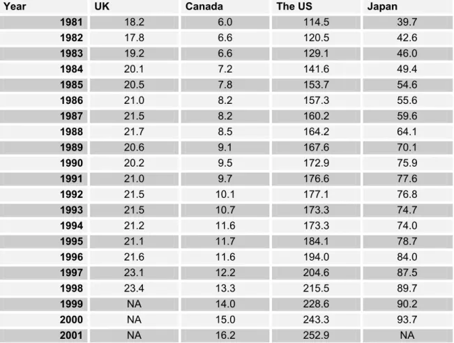
Now that the patents are our current measure of technological change, the below tables (4.1 & 4.2) reflect trends in technical changes in the United States, United Kingdom, Japan and Canada. The tables do not tell us that changes have been exponential (potentially be-cause of a significantly large residual ‘v’ discussed above), nevertheless they point to posi-tive growth.
Table 4-1 Country wise annual research expenditures in billions of USD
Year UK Canada The US Japan
1981 18.2 6.0 114.5 39.7 1982 17.8 6.6 120.5 42.6 1983 19.2 6.6 129.1 46.0 1984 20.1 7.2 141.6 49.4 1985 20.5 7.8 153.7 54.6 1986 21.0 8.2 157.3 55.6 1987 21.5 8.2 160.2 59.6 1988 21.7 8.5 164.2 64.1 1989 20.6 9.1 167.6 70.1 1990 20.2 9.5 172.9 75.9 1991 21.0 9.7 176.6 77.6 1992 21.5 10.1 177.1 76.8 1993 21.5 10.7 173.3 74.7 1994 21.2 11.6 173.3 74.0 1995 21.1 11.7 184.1 78.7 1996 21.6 11.6 194.0 84.0 1997 23.1 12.2 204.6 87.5 1998 23.4 13.3 215.5 89.7 1999 NA 14.0 228.6 90.2 2000 NA 15.0 243.3 93.7 2001 NA 16.2 252.9 NA
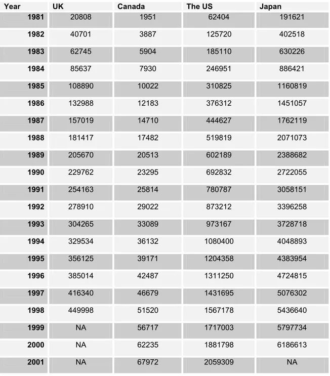
Data in table 4.2 tellsl us that Japan is leading the pack in terms of innovation. But again there is another problem with patents. Only one patent can be awarded for a single inven-tion, irrespective of its economic or technical significance. A patent for the integrated cir-cuit cannot however be compared with a patent for the toilet paper (if any such thing ex-ists). Further, threshold standard of novelty and utility imposed for granting of a single pat-ent is not too high; in fact it does not greatly differ from the standard imposed on the sci-entific journal articles of many fields (Griliches, 1990). This leads to large turnout of
appli-Patents: As the technology indicators
cations soliciting the grants, while each of them varies in their technical and economic sig-nificance from the others. Although fewer patents get applied for in the US than in Japan, one cannot conclude technological output in Japan is greater than that of the US. A quick look at table 4.1 shows us that the R&D expenditure in the US has been more than double that of Japan. And no evidence tells us that the US economy has been less innovative than Japan to account for the difference of such magnitude. This only tells us that there is a sig-nificant qualitative aspect of technical change that is not represented by the patent informa-tion; and that patents are merely a quantitative measure. The results drawn from the statis-tical analysis that uses mere quantitative measure of technical change (as represented by patents) must be interpreted with at most circumspection.
Table 4-2 Country wise annual patent stock data (obtained by compounding annual patent applications)
Year UK Canada The US Japan
1981 20808 1951 62404 191621 1982 40701 3887 125720 402518 1983 62745 5904 185110 630226 1984 85637 7930 246951 886421 1985 108890 10022 310825 1160819 1986 132988 12183 376312 1451057 1987 157019 14710 444627 1762119 1988 181417 17482 519819 2071073 1989 205670 20513 602189 2388682 1990 229762 23295 692832 2722055 1991 254163 25814 780787 3058151 1992 278910 29022 873212 3396258 1993 304265 33089 973167 3728718 1994 329534 36132 1080400 4048893 1995 356125 39171 1204358 4383954 1996 385014 42487 1311250 4724815 1997 416340 46679 1431695 5076302 1998 449998 51520 1567178 5436640 1999 NA 56717 1717003 5797734 2000 NA 62235 1881798 6186613 2001 NA 67972 2059309 NA
Patents: As the technology indicators
Since the other possible indicators of technology such as benefits from invention (captured by the labor productivity accretions) have some other variables substantially influencing them. For example, better education and health can significantly improve labor output, so this variable may not be presumed as good as patents when it comes to measuring the technical change. Similarly, research expenditure is not as good a measure as patents, since it is an input measure and not an output measure. Thus we consider the patents as the best possible option, within the current resource constrains, to proxy for technical change, tak-ing Schmookler’s lead.
Technical change in the growth models
5
Technical change in the growth models
Kurzweil’s ideas have been very intriguing but however his writings were not conventional in the sense that they were not founded on economic theory at all. He almost appeared to have had utter disdain for any such thing, as he seemed believed linear mathematics cannot capture the essence of complex non-linear system. However, we felt that ‘New growth models’ and particularly Paul Romer’s ideas on endogenous technical change is where we had to begin, not only because the work is eminently authoritative but also because it is immediately relevant. It is important to observe that we are no longer testing for the Kurz-weil’s hypothesis of exponential growth of technology; it is not possible to prove it using patents as the knowledge measure. But we try to prove the ‘standing on the shoulders’ ef-fect, which is a severely stripped down version of Kurzweil’s ideas. So the theoretical foun-dation is laid in order to fulfil this end. Section 5.1 deals with the very origins of the growth models by summarising the Solow-Swan model (1956)13. Later augmentations of early 90’s internalising technical change are dealt within section 5.2.
5.1
Solow – Swan growth model
Labour (L), capital (K) and ‘effectiveness of labour’ (A) are the inputs of this production function, and time (t) enters the function indirectly through K, L and A, i.e., output chang-es overtime only if the inputs change. Further labour and ‘effectivenchang-ess of labour’ enter the function multiplicatively, so AL is called as effective labour. This signifies that the technical progress does not enter the function as an independent determinant but as an augmenta-tion to labour. This is called as Harrod-neutral. Further, the funcaugmenta-tion reflects the homoge-neity of degree one, i.e. one unit change in inputs14 results in a unit change in the output. This also signifies the constant returns to scale in the arguments AL and K.
) , ( t t t t F K AL
Y = (5.1.1)
Rewriting equation in Cobb-Douglas form , ) ( 1 α α − =K AL Yt 0<α <1 (5.1.2)
Equation 2 again signifies constant returns to scale, with the condition ‘0<α<1’. The initial levels of capital, labour and knowledge (i.e. technology) are taken as given, and it is as-sumed that both the knowledge and labour grow at a constant rates, g and n respectively. Natural log forms of the labour and knowledge indices when differentiated over time will give us the growth rates. So the combined input of knowledge and labour will grow at the rate that is the sum of g and n.
, t nL L& = (5.1.3) , t gA A& = (5.1.4) 13 Referred in Romer, D (2001).
14 Argument ‘A’ must enter as a multiplicative of ‘L’ yielding ‘AL’ as one input, otherwise non-rivalrous
Technical change in the growth models
Since the output (Y) is dispersed for the purpose of consumption and investment (savings), a fraction of output is devoted to consumption and the remaining to investment. Solow-Swan model assumes savings as exogenous, so the fraction of output devoted to invest-ment (s) will be exogenous to the model. Devoting a unit of output will then yield a unit of physical capital. . t t K sY K& = −δ (5.1.5)
‘ δ ’ denotes the depreciation rate of capital. Now the evolution of labour and knowledge inputs become exogenous by the assumption of their non variability, and capital is also as-sumed to depreciate at a constant rate. This leaves us the evolution of capital into the pro-duction function. We however do not dwell into the details related to the dynamics of capi-tal as it is not relevant to the issue at hand.
The conclusion of the model is that the long run growth rate of the economy depends on the growth rate of technology ( A ). Again, the results of the empirical tests on Solow-Swan model are not dealt with as they are not relevant for the issue at hand.
5.2
Technical change in the New Growth Model
Technical change in this augmented Solow growth model becomes endogenous as it is dri-ven by intentional investment decisions made by profit maximising agents (Romer, P, 1990). Romer, D (2001) introduces the production function of R&D sector (of a two sec-tor economy) with out capital as
[
L t]
tt Ba L A
A& = α φ 15 (5.2.1)
Where ‘B’ is a shift parameter and ‘φ’ explains the degree of influence exerted by the knowledge stock on the output.
A model that includes capital in it will essential look like,
[
L t] [
k t]
tt Ba L a K A
A& = α 1−α φ (5.2.2)
The empirical model in this paper resembles this model without labour component. Labour has been removed to avoid the multicollinearity between R&D expenditures and research-ers head count.
If φ>0, then the number of new innovations that take place in the economy is an increas-ing function of knowledge stock, i.e. standincreas-ing on the shoulders effect. If φ<0, then num-ber of new innovations that take place in an economy is a decreasing function of knowl-edge stock, i.e. fishing in the pond effect. But usually φ is assumed by the theory as greater than zero. But there are different practically possible values that can be greater than zero. The empirical model of this paper attempts to estimate for this parameter. We consider the cases of φ equal to, greater than and lesser than one below.
15 More detailed analysis on the knowledge production function can be found in any literature on endogenous
Technical change in the growth models
If we denote growth rate of knowledge as ‘gAt’ and the growth rate of gAt as ‘g& ’, then At the dynamics between knowledge stock and the knowledge production can be depicted as follows, in Figure 5-1, 5-2 and 5-3.
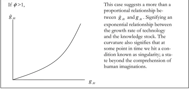
Figure 5-1 Exponential curvature
Figure 5-2 Linear curvature
The growth rate of technical change will be proportional to the stock of knowledge, signify-ing a stable linear relationship be-tween g& andAt gAt.
If φ=1, At g&
At g
This case suggests a more than a proportional relationship be-tween g& andAt gAt. Signifying an exponential relationship between the growth rate of technology and the knowledge stock. The curvature also signifies that at some point in time we hit a con-dition known as singularity; a sta-te beyond the comprehension of human imaginations. If φ>1, At g& At g
Technical change in the growth models
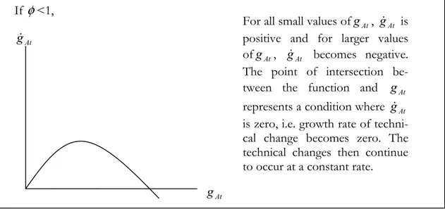
Figure 5-3 Polynomial with a neagative second order
Economists most often in their works assume the value of the parameter φ to be less than one. The empirical section of this paper perhaps makes the reasons behind this assumption more apparant.
For all small values ofgAt, g& is At positive and for larger values ofgAt, g& becomes negative. At The point of intersection be-tween the function and gAt represents a condition where g& At is zero, i.e. growth rate of techni-cal change becomes zero. The technical changes then continue to occur at a constant rate. If φ<1,
At g&
At g
Empirical analysis
6
Empirical analysis
The empirical analysis starts with the model introduction in section 6.1. Section 6.2 pre-sents results of the empirical tests and the attendant interpretations. The analysis is taken up in section 6.3.
6.1
Model for empirical examination
) , ( t t t f P R
P& = , where ‘ P ’ is the patent stock and ‘ R ’ is the research expenditures and ‘ t ’ is the time.
This functional form presents the relationships that need to be analyzed to test for the hy-pothesis. Looking from this perspective, we are looking for a positive parameter to be turned by both ‘ P ’ and ‘ R ’. But the case of ‘ P ’ is of the central interest. The function re-sembles the production function for R&D sector in the new growth model, in exception for the labor (researchers head count) component that has been removed to avoid possible multicolinearity with the R&D expenditure. R&D expenditure acts for the capital (K) that is allocated for the R&D sector, in a two sector (goods and research) economy of the new growth model. And the patent stock ‘ P ’ acts as the knowledge stock (A). The dynamics of the relationship between the growth rate of knowledge stock (gA16) and the growth rate of ‘gA’ (g&A) are the motivating factors behind building of the above functional relationship between patent stock and the annual patent applications. Now the (linear multiple) regres-sion equation to test for the hypothesis will look like,
ln zt = α + β ln Zt + δ ln Rt + εt (6.1)
ln zt = α + β ln Zt + δ ln Rt + φ ln ZtUKt + ϕ ln ZtJPt + γ ln ZtUSt + εt (6.2) ln zt = α + β ln Zt + δ ln Rt + φ ln RtUKt + ϕ ln RtJPt + γ ln RtUSt + εt (6.3) Where ‘z’ stands for annual patent applications, ‘Z’ stands for patent stock (accumulating annual patent applications), ‘R’ stand for annual research and development expenditure, ‘UK,JP,US’ are interaction dummies for United Kingdom’s, Japan’s, United States respec-tively, and ‘t’ is the time that enters through the concerned variables. Note that the vari-ables are in their natural log forms, thus expressing elasticities. To mention the differences between the three equations, it can be said that the equation 6.1 looks at the broad trend (obtained by pooling the data of all four subjects) among the subject countries on how pat-ent stock and research expenditures have influences the annual patpat-ent applications. Where as the later two equations (6.2 & 6.3) look into the contry wise effect of the same explana-tory variables on the dependent, i.e. country wise patent stock, research expenditure and annual patent applications respectively.
16 ‘
A
Empirical analysis
The introduction of the dummies became necessary due to the pooling of the data. This helps in estimating the slope parameters related to determinant variable’s patent stock and research expenditures using one single equation to calculate instead of having to run differ-ent equations for differdiffer-ent subjects.
Annual data from 1981 to 2002 is taken into consideration. Since the data is pooled, we have 84 observations; four observations are missing17 from the sourced data and are ex-cluded. There have been three other missing values18 for which average of its previous and later value has been taken as an approximate. Annual patent applications data is collected from United States Patents and Trademarks Office and World Intellectual Property Or-ganization. Patent stocks are then calculated to be the accumulating values of patent stocks. Data on research expenditures is collected from National Science Foundation of the Uni-ted States.
6.2
Results and the interpretations
Table 6-1 presents the results for the regression equation (6.1) and Table 6-2 presents the results for the regression equation (6.2) and Table 6-3 for equation (6.3). The determinant variables patent stock and research expenditure and the dependent variable annual patent applica-tions are in natural log forms. So the unstandardised coefficient values can be construed as the elasticities or growth rates of the dependant variable with respect to the growth rate of the concerned determinant19. The ‘t-values’ and ‘ p -values’ are also presented for the pur-pose of analyzing the statistical significance of the coefficient values. The model signifi-cance is predicted by the R2 value.
Table 6-1 Regression result for the equation 6.1 Determinant
Variables
Unstandardised Coefficients
t-value p -value Anova sig
Intercept -1.700 2.829 .006 .000
Zt .654 12.394 .000
Rt .383 4.197 .000
R2 .945
Observations 84 Dependent variable: zt
17 Annual patent applications data and R&D exp for UK missing for years 1999, 2000, 2001, for Japan: 2001. 18 R&D expenditure data.
19 For the dummies, their slopes need to be summed up with the slopes of the primary variables to obtain the
Empirical analysis
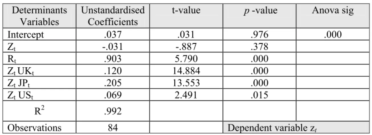
Table 6-2 Regression result for the equation 6.2 Determinants
Variables
Unstandardised Coefficients
t-value p -value Anova sig
Intercept .037 .031 .976 .000 Zt -.031 -.887 .378 Rt .903 5.790 .000 Zt UKt .120 14.884 .000 Zt JPt .205 13.553 .000 Zt USt .069 2.491 .015 R2 .992
Observations 84 Dependent variable zt
Table 6-3 Regression result for the equation 6.3 Determinant
Variables
Unstandardised Coefficients
t-value p -value Anova sig
Intercept .454 .394 .694 .000 Zt .063 1.702 .093 Rt .756 4.735 .000 Rt UKt .138 18.386 .000 Rt JPt .257 16.049 .000 Rt USt .086 2.926 .004 R2 .994
Observations 84 Dependent variable: zt
All the coefficient values reported in the above tables are statistically significant, in excep-tion for the patent stock (i.e. of Canada, in the model with interacexcep-tion dummies) in Table 6-2. The t-values are above their cut off level of |2| and in cases where they are below |2| their p -values show that they are at least significant at 10% level. The goodness of fit or the explanatory power of the models, which is shown by the R2 values, is also highly sig-nificant at .992 for the regression equation (6.2) and .994 for the regression equation (6.3). This means the respective models are explaining 99% of the variance in their dependent variables. So the results predicted by the model can be depended upon. Further, Anova significance is also high at .000.
As mentioned earlier, since the variables in the regression equation are in their natural log forms, they express elasticities or growth rates. That is, a percent growth in the explanatory variable leads a certain percent (represented by explanatory variable’s coefficient) change in the dependent variable. The coefficient values of patent stock and research expenditures stand for the elasticity of the Canadian annual patent applications turn out with respect to the Cana-dian patent stock and the CanaCana-dian research expenditures. In order to calculate the elasticities (slope) of UK’s, Japan’s and United States’ dependent variables with respect to their de-terminant variables, the coefficients of the respective country dummies are to be summed up with the coefficient values of patent stock and research expenditures respectively. So the UK, Japan and United States elasticities will look like the results in Table 6-4.
Empirical analysis
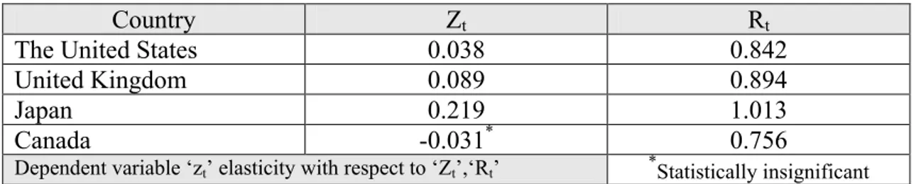
Table 6-1 Elasticities
Country Zt Rt
The United States 0.038 0.842
United Kingdom 0.089 0.894
Japan 0.219 1.013
Canada -0.031* 0.756
Dependent variable ‘zt’ elasticity with respect to ‘Zt’,‘Rt’ *Statistically insignificant
We have all the countries registering statistically significant coefficient values for patent stock as determinant variable. A percent increase in the patent stock of the US leads to 0.04% in-crease in the annual patents turn out. The English annual patent applications grow 0.09% in re-sponse to a percent increase in UK’s patent stock. Japanese show the most robust rere-sponse so far with their annual patent applications growing at 0.22% in response to a percent change in their patent stock. Canada is the only exception to the trend that has been consistently and correctly a positive sign. It shows a negative sign. A percent increase in Canadian patent stock leads to a 0.04% decrease in the annual patents turn out. This is bizarre and of course not quite literally true. Further it is statistically insignificant, with the t-value of -.887. This means that the coefficient is not significantly different from zero, thus leaving us nothing to infer from the result. Although we try to pronounce a reason for this wrong sign, the re-sult need not confound us since it can potentially be wrong.
The determinant variable research expenditure has given us correct signs and all values are sta-tistically significant, so did its respective dummies. A percent increase in the U.S research ex-penditure leads to 0.84% increase in the annual patent applications turn out. UK reports a little higher figure at 0.89%. Japan has the highest elasticity for the annual patent applications turn out with respect to its research expenditure at a little more than 1%. Canada registers the least of all the figures; her annual patent applications are growing at 0.76% in response for a percent increase in her research expenditure.
6.3
Analysis
Giving consideration for the statistical result derived from a model that does not include country dummies (equation 6.1) is both technically feasible and is necessary in this case. This indicator tells us the over all pattern in the relationship between the patent stock and the annual patent application turn out. And this is the central question of this paper. So we take a look at the results of the regression models with country dummies as well as the re-sult of one of the stripped down version of these models. The statistical ambiguity (see sta-tistically insignificant value for Zt for equation 6.2, shown in table 6.2) related to patent stock coefficient value (attributed to Canadian data) arises from the split incurred by the country dummies in what essential is a pooled data. The usage of such country dummies is neces-sary in order to derive results that can be individually attributed to each of our subject countries. This in fact is the essence of the regression equations 6.2 and 6.3.
If we consider the model (equation 6.1) that excludes the country dummies, the patent stock variable returns a statistically distinct answer (ref: table 6.3). The coefficient value of this variable, endorsed by a t-value of 12.394 (and a p -value of .000), stands at 0.654. Inter-preted in terms of annual patent applications elasticity with respect to patent stock, it tells us that a percent increase in patent stock leads to 0.65% increase in annual patent applications. This is a non-ambiguous ‘yes’ to the hypothesis of ‘standing on the shoulders’ effect, with a good
Empirical analysis
degree of certainty at least to the subjects that we investigate. The stock of inventions posi-tively influencing the rate of innovation is a reflection of the path dependent aspects of technical change that Rosenberg (1994) discusses, a summary of which is presented in sec-tion 2.
There is a very strong relationship between the research expenditure and the patents stock’s influence on the rate of patents turnout. Although there is proof that the patent stock positively influences the rate of patents turnout, such causality cannot run directly. One of the fundamental channels through which the causality runs is R&D expenditure. This can be very intuitively reasoned. If we do not invest in the research, how can we ever make use of any positive influence that our knowledge stock might have on further innova-tion? The patent stock does not passively bring about innovation; it is active employment of the stock via capital intensive research that brings about innovation. As Griliches (1990) pointed out, the volume and duration of research expenditures do have profound implica-tions on patents turn out. The more we invest, the more we can capitalize on the positive relationship between the knowledge stock and innovation. This relationship might explain Canadian patent stock’s bizarre coefficient value.
Theoretically, we expect the sign of the coefficient value for patent stock for all the countries to be positive. It is positive in all the cases in exception for Canada, which is statistically in-significant. And a distinct pattern that must be noted is the Japanese patent stock returned a coefficient value that is statistically significant and more than double that of its counter-parts. The annual patents turn out, as shown in graph 4.1 , of Japan is also substantially higher than the other countries. This shows us that Japan has been highly productive in patenting. But these numbers are however not enough to say that Japan is more innovative than the US. This difficulty results from another peculiarity of the information embedded in a patent. As stated earlier, irrespective of the technical and economic significance of an invention it can be offered only one patent. For example, patent for the thermoelectric module20 differs enormously from the patent for an undershirt in its technical, economical significance and also by its ability to bring about further innovation in its own stream or in others. It is a very huge task to assign each and every patent some kind of index to measure its significance and ability to bring out further innovation. This form of data, to our best knowledge, is unavailable. And without such information we cannot actually conclude that Japanese economy is more innovative than that of the US just basing on the patent applica-tion numbers. However, if we consider the labor productivity as a measure we might per-haps make more sophisticated speculations on the innovativeness of the economy (note that innovation ultimately manifests in productivity accretions). As the chart in appendix 1 shows, the Japanese productivity levels hover somewhere around 75% of the US levels, both in terms of the GDP per person employed and GDP per hour worked. This tells us that the US economy is more productive than Japan, and that patent applications turn out alone cannot be construed to suffice for landing on conclusions about relative innovative-ness of the economies.
Further, the R&D response parameter of Japan is also greater than that of the US. As shown in table (6-4) Japan registers 1.013 and the US registers 0.842. That put in terms of elasticities gives us, a percent change in the Japanese research expenditure leads to a little more than a percent change in Japanese patent output, and a percent change in the US re-search expenditure leads to 0.84% change in US patent output. This means Japanese R&D
Empirical analysis
sector is more productive, for capital as the factor. This conclusion put together with the previous observation that US labor productivity levels are higher than Japan gives us enough space to speculate that Japanese research primarily goes into development research, which on average then can be concluded to be not technically as sophisticated and less capital thirsty than an average US research project. Note that US research expenditure is twice as large as Japan’s (ref: table 4-2). For instance, major part of Japanese research ex-penditure goes to projects in electronics and information systems, where the patents are easier to obtain than, say, in pharmaceutical projects (Piling, D 2005). If it holds that the US ends up spending more on projects that are more complex projects (for e.g. large scale defense avionics projects or drug research), as it seems, then although US is more innova-tive than Japan, it might end up less producinnova-tive than Japan when it comes to patents. The difference in one county’s patent stock coefficient value (as well as that of R&D expendi-ture paratmeter) from the others may be explained by two primary reasons among others. 1. The path dependency in the research activities, i.e. Japan investing more in electronics where the patents are easier to obtain and the US investing more in much complex projects such as medical research (Piling, D 2005). 2. Allocation of resources in the economy to the R&D sector. If a country’s research flourishes in mature technologies, then there will be more patents applied for (and more patents per dollor invested), since understandably the process of differentiation must be relatively easier compared to the process of creation of new technologies right from the scratch. Further, the more a country invests in the re-search, the better position it will be in exploiting the benefits that the existing knowledge stock offers. So it can be argued that the estimator for patent stock might return a higher value if more capital is allocated to R&D sector. To sum up, the discrepancies, that we see in terms of differences in patent stock co-efficeint values of individual countries, evolve overtime due to the differences in research pathways that an individual country pursues. Another trend that is esoteric in the test results is the Canadian patent stock’s return value. Its sign is negative and is statistically insignificant. It is recorded to be -0.031. This suggests ‘fishing in the pond’ effect. But such a notion leads to a logical conclusion, i.e. an eventual exhaustion of the pond. That, however, is not the case. The scientific or technological frontier for Canada is the same as to that of the US, Japan or UK. When a general tendency of the variable annual patent applications seems to be growing in response to patent stock, it is improbable that Canada is proving that technological frontier can be exhausted. But there are other observations that can help to explain this negative sign. As stated earlier in this section, there is a strong relationship between the R&D expenditures and the patents stock’s influence on patent output. Table 4-2 shows that Canadian research expenditure has been relatively stagnant at the level of 10-15 billion USD along the range of observations in this study, although such investments show an impressive coefficient value of 0.756 (i.e. 75% elasticity). So it can be reasonably stated that the anomalies in the resource allocations for the R&D sector in Canada is showing us the negative relationship between the patent stock and annual patent applications.
As stated earlier, the wrong sign that Canadian patent stock returned need not be that puz-zling since it is statistically insignificant and could potentially be wrong. This might be be-cause of data shortage and the relatively slow pace of changes in the variable.
Conclusions
7
Conclusions
Many economists assume the ‘φ’ parameter in the knowledge production function of the endogenous technical change models (ref: theoretical review) to be greater than zero and less than one. This assumption seems to be supported by the empirical estimates of the function with patents as the proxy for knowledge or technology. This in fact is exactly what the models used in this model are extrapolating. A reference to Table 6-1 will shows us the ‘φ’ parameter estimated to be less than one, at 0.65. Thus we state that our finding is in line with the mainstream economic expectations related to this issue of knowledge dynam-ics.
The purpose of the paper, which is to demonstrate (generally) positive relationship be-tween the technological stock and the rate of technical change, stands justified in the light of statitstical results. Discrepancies do exist when comparing the coefficients of the differ-ent countries, i.e. the variation in their coefficidiffer-ent values, nevertheless the signs are positive as expected. An interesting observation that can be made at this point is as follows. The annual patent applications themselves embody the technical changes, so the variable ‘zt’ in natural log form returns the rate of technical change. Any positive rate of technical change inresponse to the given technological stock implies accelerating rate of technological change, i.e. the rate of technological change is itself positively growing.
Further, the advantages provided by the knowledge stock to attain better rates of technical changes can only be attained through more active research participation, which inevitable results in greater R&D expenditures. One might question such conclusion by taking a skim at the data on patent applications and R&D expenditures. For example, the US R&D ex-penditure is almost twice that of Japan but at the same time number of Japanese patent ap-plications is nearly twice that of the US. So we do not mean to contend that increased R&D expenditure necessarily results in increased patent applications but it is fair to expect that such an increase will result in greater volume of technical changes (that perhaps can be captured more accurately by other variables, such as total factor productivity). The example considered above points to the possibility that the residual discussed by Griliches (1990) in equation (4.2) must be significantly large. This lack of proper feed on the technical and economic significance of an innovation in the information embedded in a patent is the main reason leading to possibly large residual value .
Although one cannot suggest which technological pathway (one in mature or complex state) a county should choose to pursue, it can be said that more research investments will certainly help exploit any positive influence that the existing stock of knowledge has on the pace of technical changes. Then it is an imperative that the governments must actively pur-sue policy that will allocate more resources to R&D sector. Technological pathways, which show up as patterns of concentration and specializations of certain industries in certain contries, is better left free of policy interventions and to the market forces, as it is now. As far as the research related to similar models trying to estimate the relationship between the technological stock and the rate of technical changes, it is suggested that total factor productivity or some arrangement of multifactor productivity be used to proxy for the technological changes. We believe that broder measure of productivity levels may have more information feed on technological changes than annual patents turnout. Although the models might evolve to be much more complex, the anticipation is that they will be sur-rounded by less restrictive settings, thus giving us more reliable numbers to read.
Appendices
References
Callan, Eoin (2005), “Cancer drug divides opinion”, The Financial Times.
Griliches, Zvi (1990), “Patent statistics as economic indicators: A survey”, Journal of economic literaure, American Economic Association.
Griliches, Zvi, Nordhaus, William D., Scherer, F.M., (1989), “Patents: Recent trends and puzzles”, Brookings papers on economic activity, The Brookings Institution, USA.
Harraway, Donna, “Modest_witness @ second millennium”, in The social shaping of technology, second edition, Open University Press, Philadelphia, USA.
Intel Corporation (2005), http://www.intel.com/technology/silicon/mooreslaw/index.htm, intel.com.
International Labor Organization (2005), world wide web resources, ilo.org.
Jones, Charles I. (2004), “Growth and Ideas”, NBER working paper 10767, National Bureau of Eco nomic Research, USA.
Kurzweil, Ray (2001), “The law of accelerating returns”, kurzweilai.net.
Mackenzie, Donald and Wajcman, Judy (1999), The social shaping of technology, second edition, Open University Press, Philadelphia, USA.
Mackintosh, James (2005), “Ideas that drive GM’s shareholder value”, The Financial Times Maddison, Agnus (1982), Phases in capitalist development, Oxford University Press, UK. Micron Technologies Inc (2005), http://www.micron.com/k12/semiconductors/history.html,
micron.com.
Moravec, Hans (1993), “The age of robots”, Robotics Institute, Carnegie Mellon University, USA.
Piling, David (2005), “Creative models shaped by education”, The Financial Times.
Romer, David (2001), Advanced Macroeconomics, second edition, McGraw Hill higher educa-tion, USA.
Romer, Paul M. (1990), “Endogenous technological change”, The journal of political economy, The University of Chicago Press, Chicago, USA.
Rosenberg, Nathan (1994), Exploring the black box: Technology, Economics and History, University of Cambridge Press, UK.
Schumpeter, Joseph A. (1976), Capitalism socialism & democracy, George Allen & Unwin (publishers) Ltd, UK.
Simpson, David (2000), Rethinking Economic Behaviour: How the economy really works, Macmillan press Ltd, UK.
Solow, Robert M. (1987), Prize Lecture in memory of Alfred Nobel, The Nobel Foundation.
Appendices
The National Science Foundation (2004), The science and engineering indicators, USA. Nsf.gov.
The United States Patents and Trademark Office (2003), The annual patent statistics report, USA. Uspto.gov.
The World Intellectual Property Organisation (2005), The annual industrial property statistics. Wipo.int.
The Nobel Foundation (2005), http://nobelprize.org/economics/laureates/1987/solow-lecture.html, nobelprize.org.
Appendices
Appendix 1. Productivity chart
Figure A-1 shows the per capita output in terms of labour hours and per capita output in terms of labour units.
Figure A-1 Productivity chart
Appendices
Appendix 2. Microprocessor, Scientific paradigms,
path dependent technical changes
21In 1948, a Nobel winning (1956) invention ‘the transistor’22 was born in Bell telephone labs, which transformed the world of computing23 the way we have it today. Its invention by the three physicists, W. Shockley, J. Bardeen, and W. Brattain, had opened up a scien-tific paradigm, within which we had seen decades of technical change. Let us very briefly examine how path dependent technical changes occur with in the bounds (which are well defined in this case) of a scientific paradigm. The transistor at the beginning used to be made from a ‘semiconductor material’24 called Germanium, but it was later given up for a better replacement25, another semiconductor material called Silicon. However, building sili-con-based transistors one by one from individual semiconductor material had become a very challenging task as the need for more complex, and large number of, electronic cir-cuits grew. Eventually, the industry needed better science to build better (smaller and faster) processors. Thus the birth of microprocessor, whose invention is the very reason why we today have ubiquitous personal computing. It is based on an architecture built us-ing Integrated Circuits (IC). These ICs (for that matter, even the large scale and very large scale integrations) are basically the collection of transistors. Instead of making transistors one by one, several of them were made out of one piece of semiconductor. This technique of placing large number of components on one tiny chip creates Integrated Circuit. Jack Kilby of Texas Instruments and Robert Noyce of Fairchild Camera were awarded Nobel in physics in 2000 for this invention (1959). Before these transistors came into the existence, vacuum tube triodes were used for similar purposes. In a Nobel winning work, Joseph John Thomson was one of the earliest to build a vacuum tube, which resulted in the dis-covery of electron, for which Thomson was awarded the prize in 1906. A good example for the tube is Edison’s light bulb (with two electrodes). However, the vacuum tube leaked and the metal that emitted electrons in vacuum tubes burned out, the tubes also consumed large amount of energy and space and were very inefficient as the electric circuits became complicated (Haviland, 2001). This very drawback of vacuum tubes lead to the invention of a technique to conduct electrons on solid materials, like semiconductors.
These transitions from vacuum tube triodes to transistors; transistors to integrated circuits can be viewed as shifts in scientific paradigm. The shifts from one paradigm to another oc-cur when a scientific paradigm is exhausted. When vacuum tubes could not be pushed any further, as the need for more complicated electronic circuits manifested, that lead to a shift
21 Technical information in this section is very general, and can be availed using encyclopaedias or online
se-arch engines. Technical definitions are loose, since the purpose is only to give an example for scientific pa-radigm and path dependent technical changes.
22 The transistor is a solid state electronic device used for the purpose of amplification of weak signals by
en-larging their voltage, it is also used for switching purposes in digital devices, i.e. switching between 0 and 1 or between ON and OFF conditions.
23 Broadly speaking, the whole field of electronics was deeply shaped by the invention of the transistor. 24 Materials such as Zinc, Germanium or Silicon are called using a generic term semiconductor, because
changes in their properties caused by the fusion of minute amount of impurities leads to the difference be-tween conducting and non-conducting of electric current (Mircon Technologies, 2005).
Appendices
to transistors. And when transistors seemingly hit their limits they were given up for ICs. However, we must observe that exhaustion of a scientific paradigm is totally different from the notion of an exhaustion of scientific frontier. As long as the progressive shifts (such as vacuum tube to transistor to IC) are feasible, scientific frontier cannot be exhausted. Fur-ther, we can also observe that scientific changes (different from technical changes) are themselves path dependent.
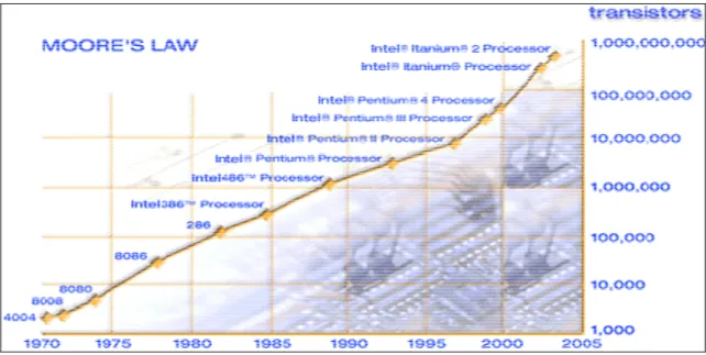
Since the invention of the IC, we had seen decades of technical changes to improvise the performance of the microprocessor. The scientific paradigm that came into existence due to the invention of IC allowed for years of technical progress with in its bounds. These technical changes can be well-explained using Moore’s Law26.
Figure A-2 Path dependent technical changes Source: Intel Corporation, Intel.com
As the graph shows, when Intel released it 4004 processor in early 70’s, the chip was made out of approximately 3000 transistors. By the time Intel released 8080 in ´74, the chip con-sisted more than 8000 transistors. The chip kept on adding more transistors while it itself was shrinking in size, as shown in the progression in the graph. By early 90’s when Intel re-leased the first version of the now popular Pentium, the chip contained a few million of the transistors and it is close to a billion transistors in Intel’s latest Itanium. It is speculated that limits of this paradigm will be reached in the later half of the next decade, when the chip cannot accommodate any more transistors. The constraints imposed by the physics may not even allow latest of the nano-technologies to push the relevance of the Moore’s law any further into the future. However, Intel and the other chip manufacturers have been re-searching on new architectures in order to allow for technical changes to continue. One such innovation had found its way into the markets already; it is the Intel’s dual core proc-essor27. Intel’s website claims that by 2015 a processor will accommodate a few hundred
26 In 1965, Intel’s co-founder Gordon E. Moore prophesised that the number of transistors on a chip
(mi-croprocessor) will double roughly every two years. This prophecy was given the name ‘Moore´s Law.