View of A Nonlinear Dynamic Model Applied to Data with Two Times of Measurement

2016, 2(1–2)

Published by the Scandinavian Society for Person-Oriented Research Freely available at

http://www.person-research.org

A Nonlinear Dynamic Model Applied to Data with Two Times of

Measurement

Anton Grip

, Lars R. Bergman

2_{Department of Psychology, Stockholm University}

Contact

gripanton@gmail.com

How to cite this article

Grip, A., & Bergman L. R. (2016). A Nonlinear Dynamic Model Applied to Data with Two Times of Measurement. Journal of Person-Oriented Research, 2(1–2), 56–63. DOI: 10.17505/jpor.2016.06

Abstract: A good model of developmental phenomena should not only “explain” the data in the sense that the model is not falsified by the data but it should also be built on the basic theoretical assumptions about the process under study. This is often not the case when standard statistical models are applied to developmental data. An alternative is then to apply nonlinear dynamical system modeling. This approach is followed in the article and it is illustrated by a provisional model of the development of boys’ problem behavior between the ages 10 and 13. The underlying interactionistic theory of development was mirrored in a nonlinear model that predicted outcomes marginally better than a standard regression model. It is pointed out in the article that it might be possible to use nonlinear dynamic system modeling also in contexts where data are available only from a few measurement occasions.

Keywords: Dynamical systems, developmental science, adjustment problems, longitudinal

Introduction

During the last decades, a discontent has grown among many leading researchers within developmental science (DS) concerning a mismatch between, on the one hand, key tenets of many theoretical conceptualizations and, on the other hand, common approaches taken in empirical re-search to address scientific questions within the field of DS. These researchers include, for instance, Robert Cairns, Gilbert Gottlieb, and David Magnusson. Part of their dis-content lies in that these common approaches do not al-low the researchers to interpret their findings in relation to modern DS theories, which emphasize dynamic interac-tions and whole system properties (Bergman & Andersson,

2010;Bergman & Vargha,2012).

From a methodological standpoint, standard current sta-tistical methodological practices have also been criticized for

1. Not taking into account whole system properties as

re-flected by patterns of functioning (Bergman & Mag-nusson,1997).

2. Producing findings that are only interpretable at a group level, not at the individual level (Molenaar,

2004;Nesselroade & Ram,2004).

Several researchers have pointed to the potential of mathematical models for nonlinear dynamic systems (NO-LIDS) as vehicles for carrying out research in DS. NOLIDS match fundamental requirements of DS theoretical propo-sitions in that they are process oriented and can accom-modate nonlinearities, interactions, bi-directional causal-ity, and change on a continuous scale. Properties of a suc-cessful model are also interpretable in relation to typical DS theoretical conceptualizations. NOLIDS has for a long time been a mainstream methodological approach within the natural sciences (weather prediction, prediction of number of individuals of a certain species in an eco-environment, etc.) and it is now making its way into developmental

sci-ence (see, for instance,Boker,2002;Granic & Hollenstein,

2006;Kelso,2000).

Most commonly, NOLIDS is applied to time-series data in an experimental context but such models are more widely useful. In this article, an example of the use of a NOLIDS model is given when data from only two time points are analyzed; an unusual setting for such models1_{. It should be} pointed out that the NOLIDS model presented in this article is assumed to be common for all individuals and that it may or may not hold at the individual level (cf. point (2) above). However, whole system properties are central in this type of model and it allows for attractors to emerge (cf. point (1) above).

Aims

The broad aim is to exemplify a NOLIDS approach to the study of development within a DS framework where data are available only from a few measurement occasions. Fur-ther, model building and the search for a good model is dis-cussed from a natural science perspective, offering a partly different perspective on these issues to what is common in the context of psychological research. NOLIDS is con-trasted to a standard statistical modeling approach using regression analysis and pros et cons of the two approaches are discussed. To make the presentation more concrete, an example is presented where empirical data of the develop-ment of problem behaviors are analyzed, using both types of modeling.

The NOLIDS model we present should be regarded as an illustrationof the possibilities of using this approach in DS. It should not be regarded as giving a contribution to the literature about understanding the development of boys’ problem behavior.

A Note on Dynamic Living Systems and Their

Modeling

In the following, a short introduction to some aspects of the modeling of dynamic living systems is given as regarded from a natural science perspective (for an overview from a behavioral science perspective, seeGranic & Hollenstein,

2006).

Systems in living organisms tend not to be successfully modeled in the same way as most physical systems can be modeled. For instance, different organisms can, under the same conditions, be in different stable states (attractor states) and identical initial states can lead to different later states of the system. There also tend to exist both attractors and instable states that are repellent. For this to happen, and for the system to be flexible so as to adjust to a chang-ing environment, processes that counteract each other must be incorporated in the system. A system characterizing a living organism is often in a meta stable state, meaning a state that is attracted to a certain state but without that state being a “true” attractor or stable state. This leads to

1_{This article is largely based on a B.A. thesis by Anton Grip (Grip,2002)} and some of its findings have been discussed byBergman and Vargha

(2012) in relation to the problem-method match.

that the system’s behavior is characterized by moving close to some state but at the same time is free to move within its neighbor region. The brain is one example of a system in a meta stable state (Kelso,2000). If the attractor states were too strong, the brain network would be captured in a collective stable state, leading to inflexibility. On the other hand, without any weak attractors, the behavior of the net-work would be uncoordinated, perhaps even chaotic. A sys-tem being in an unstable state can be attracted to different semi-stable states, depending on infinitely small variations in the unstable initial state. This type of behavior is called bifurcation (Boyce & DiPrima,1997) and in this way self-organizing systems of living organisms can achieve flexibil-ity.

According toKelso(2000), the following properties char-acterize systems of living organisms and should be taken into account when they are modeled:

• Synergy. The systems parts are connected to form functional units, optimized to function together. This might lead to that system behavior can be understood in spite of an incomplete knowledge of all its parts. • Multifunctionality. In a given situation, many types of

system behavior can be generated by the same parts of the system.

• Stability. The ability to show the same system behavior in many different situations.

• Function variance. The ability to achieve the same goal by using different parts of the system in different ways. • Flexibility. The ability to change system behavior to meet new environmental demands. This can be looked at as a selection mechanism (an optimization) that chooses the simplest or most stable behavioral path that leads to the goal.

Differential equations are almost always used in the mathematical modeling of a dynamic system. The equa-tions describe system change in continuous time and the types of differential equations used in this article were de-veloped already in the 18th century by Lagrange (seeBoyce & DiPrima, 1997). Using this approach, it is possible to model most of the characteristics of a system that describes a living organism. If stochastic components were added to the model, this match could be further improved. However, this is complicated and it was not attempted in this article: the differential equations that are presented are determin-istic.

Central to any modeling approach is the issue of what constitutes a “good” model and how the best model can be chosen from a set of possible models. This issue has, of course, been much discussed in psychology and a number of common procedures have emerged (for instance, focus-ing on model fit or comparative model fit). However, in the natural sciences, models are usually evaluated and se-lected in different ways to what is common in psychology. For instance,Peterson and Eberlein(1994) suggest the fol-lowing criteria for deciding if a mathematical model of a phenomenon is a good model:

1. The extent to which the model mirrors the different parts of the theory.

2. How well the model fits to data.

3. Whether the model behaves “reasonably” when thought experiments are performed for extreme situa-tions.

4. Whether the model allows for statements about situa-tions that are far outside the data space observed. 5. Whether the model is sensitive to parameter changes. Two additional criteria for a good model should be noted (Casti,1989):

6. The explanatory power of the model.

Explanation is then seen in contrast to mere description of system behavior. In fact, Casti distinguishes between what he calls a model of a system and a simulation of a system. A simulation can only predict data while a model also to some extent explains the studied phenomena and addresses the question “why”. This implies model properties are inter-pretable in terms of the theory-phenomena relationships.

7. Simplicity.

Any set of data can be perfectly described by a model that is sufficiently complex but such a model is only a simula-tor. A simpler and “real” model that has explanatory power and can be generalized to hold for other data sets is often preferable, although its predictive power is inferior to that of a complex simulator.

For a more thorough discussion of what is a good model, regarded from a philosophical perspective, it is referred to

Needham(2001).

An Empirical Example: Growth of

Ad-justment Problem Behavior

Theoretical Conceptualizations and Scientific

Problem

Within the longitudinal research program “Individual De-velopment and Adaptation” (IDA;Magnusson,1988), the study of problem behavior, its development, and its roots, has been an important research area. The IDA theoreti-cal framework and empiritheoreti-cal findings have also led to a number of theoretical conceptualizations about the process of adjustment problem development (Magnusson, 1988). The broad theoretical framework has been the holistic-interactionistic research paradigm and its formulation in the person-oriented approach (Bergman & Magnusson,

1997). Hence, it is strongly DS-oriented. In the empiri-cal example presented here, we are interested in one as-pect of the study of adjustment problem behavior, namely the growth of boys’ externalizing problems as regarded in the context of linked internalizing problems. With the pur-pose to demonstrate a NOLIDS model, a “mini system” was defined consisting of boys’ externalizing problems and the

two internalizing adjustment problems distress and timid-ity. This mini system was assumed to have the process prop-erties previously described. Eight tentative specifications of the system properties were made based on the IDA re-search:

1. Distressed boys tend to have increased externalizing problems.

2. Boys with externalizing problems tend to have prob-lems with peer relations and to experience negative feedback, which leads to increased distress.

3. Boys with pronounced externalizing problems easily form bonds to other maladjusted boys, forming a sub culture that is conductive to stabilization or even ag-gravation of these problems. On the other hand, boys with only weak tendencies to externalizing problems will experience a pressure from their environment to conform, which often leads to decreased externalizing problems. This is an example of the problem gravita-tion hypothesis as formulated byBergman and Mag-nusson(1997).

4. For boys without externalizing problems but who are distressed, there is also, in contrast to point 1 above, a tendency for self-healing.

5. A boy with extreme externalizing problems will quickly become more distressed.

6. Timidity is largely time-invariant and is regarded as a stable personality characteristic.

7. Boys who are very timid are highly responsive to crit-icism, if they exhibit externalizing problem behavior, which buffers against the growth of such problems. 8. Boys who are timid run the risk of developing

in-creased distress.

In the NOLIDS model described below, we strived to in-corporate these eight specifications, as well as general pro-cess properties of the type earlier described. The focus is on understanding the growth of externalizing adjustment problems as it evolves in the context of the two internaliz-ing adjustment problems included in the mini system.

Sample and Variables

Longitudinal data were used about boys’ adjustment prob-lems, measured by teachers’ ratings at age 10 and at age 13. Data were taken from IDA and only boys with complete data were included in the study (n= 452). The following teachers’ ratings were used:

• Aggression • Motor restlessness • Concentration difficulties • Low school motivation

• Timidity (shyness, inhibition)

All rating scales were originally graded 1− 7 with “1” in-dicating a complete absence of the problem being rated, “4” indicating what is regarded by the teacher as a “nor-mal” level of the problem, and “7” indicating an extreme presence of it. The rating scales were transformed to better reflect the degree of “real” problems, i.e. problems beyond what is the norm for children (see Table 1). Previous stud-ies within IDA indicate that the first four teachers’ ratings presented above can be regarded as belonging to the same factor, labeled Externalizing problems. Hence, for simplic-ity, in this study, instead of these four teachers’ ratings, we used only the average of them (based on the transformed ratings).

Table 1. Transformation of ratings used in this article.

original ratings transformed ratings

1-4 0

5 1

6 2

7 3

To summarize: Three scales were included in the analy-ses, namely Externalizing problems (E), Distress (D), and Timidity (T). Each was measured at age 10 and again at age 13, hence six variables were analyzed. When neces-sary, the age at the time of measurement was added after the letter indicating the scale to specify the variable (e.g. E₁₀is Externalizing problems measured at age 10).

The Linear Model

The linear model we first used was a simple multiple re-gression model (MRA model) for predicting Externalizing problems at age 13, using the three adjustment problems measured at age 10 as predictors:

E₁₃= A + BE₁₀+ C D₁₀+ DT₁₀ (1)

To make the linear model somewhat more comparable to the NOLIDS model described below, a more elaborated regression model was also fitted to the data. Starting from Model (1), a regression analysis was performed to inves-tigate whether the regression model’s predictive power is increased when nonlinear terms are added to the equation. Six terms were included in a stepwise analysis: The square of each of the three adjustment problems at age 10 and the three centered interaction terms between each pair of adjustment problems at age 10. To a very limited extent, these terms also relate to some of the theoretical expecta-tions of the system properties (e.g. the square of E₁₀relates to Specification 3).

The NOLIDS Model

Based on the eight tenets about the developmental process of problem behavior that were described above, a NOLIDS model was constructed. One standard model was chosen

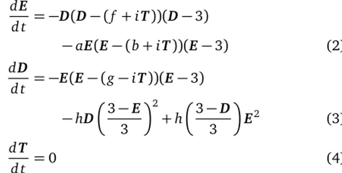
that reasonably well fitted the tenets. The model was de-fined by the following set of differential equations (Bold= variable): d E d t = −D(D − (f + iT))(D − 3) − aE(E − (b + iT ))(E − 3) (2) d D d t = −E(E − (g − iT))(E − 3) − hD ₃ − E 3 ‹2 + h3− D 3 ‹ E2 (3) d T d t = 0 (4)

where the constants a−i are parameters to be estimated by fitting the model to data. The parameters were constrained to have positive values.

It is possible that the model generates values for Externalizing problems or Distress outside the range 0− 3. Such a value is set to the closest extreme value (i.e. 0 or 3).

Description of the differential equations: −D(D − ( f + iT ))(D − 3) :

The first of the two terms in Equation (2) reflects Point 1 from the theory (1. Distressed boys tend to have in-creased externalizing problems). If Distress is larger than f + i∗Timidity, the whole factor will be positive, contribut-ing to higher externalizcontribut-ing problems.

−aE(E − (b + iT ))(E − 3) :

The second term in Equation (2) corresponds to Point 3 from the theory (3. Boys with pronounced externalizing problems easily form bonds to other maladjusted boys, forming a sub culture that is conductive to stabilization or even aggravation of these problems. On the other hand, boys with only weak tendencies to externalizing problems will experience a pressure from their environment to con-form, which often leads to decreased externalizing prob-lems.). In similarity to the terms described above, it is also a third degree polynomial that is negative for val-ues of Externalizing problems less than b+ i∗Timidity and positive for values of Externalizing problems larger than b+ i∗Timidity. It contributes to that boys with externaliz-ing problems will have even larger such problems but those with less externalizing problems will have decreased prob-lems. Hence, this term describes problem gravitation.

−E(E − (g − iT ))(E − 3) :

The first term in Equation (3) is of the same type as the one described above and it corresponds to Point 2 from the theory. (2. Boys with externalizing problems tend to have problems with peer relations and to experience negative feedback, which leads to increased distress.) It contributes to an increased distress if the boy has externalizing prob-lems larger than g− i∗Timidity.

−hD ₃ − E 3 ‹2 :

The middle term in Equation (3) corresponds to Point 4 from the theory (4. For boys without externalizing prob-lems but who are distressed, there is also, in contrast to point 1 above, a tendency for self-healing.). It contributes to a decrease in Distress if the externalizing problems are small. h _{3− D} 3 ‹ E2:

The last term in Equation (3) corresponds to Point 5 from the theory (5. A boy with extreme externalizing problems will quickly become more distressed). It contributes to an increased Distress if Externalizing problems are large.

d T d t = 0 :

Equation (4) corresponds to Point 6 from the theory (6. Timidity is largely time-invariant and is regarded as a stable personality characteristic). That T:s time derivative is zero means that Timidity is regarded as a stable characteristic that is not time dependent.

Point 7 from the theory (7. Boys who are very timid are highly responsive to criticism, if they exhibit externalizing problem behavior, which buffers against the growth of such problems) is represented in the model by its flexibility in changing factor contributions in the equations timidity are part of. This means that the value is changed for when the term switches from being negative to positive. An ex-ample: The second term in Equation (2) describes problem gravitation in Externalizing problems. The tipping point for having increased or decreased values is determined by the term−(b+i∗Timidity) where b and i are constants that are adjusted for maximum model fit. If Timidity is large, this tipping point will be large, i.e. externalizing problems must initially be present for them to grow. On the other hand, if T = 0 the tipping point is at a lower level of Externalizing problems. In this way, boys characterized by a high degree of Timidity will be subjected to a protective effect against developing pronounced Externalizing problems.

Point 8 from the theory (8. Boys who are timid run the risk of developing increased distress) corresponds to the term −(g − i∗Timidity) in Equation (3). If a boy is high in Timidity he will tend to have increased Distress for low levels of Externalizing problems.

Description of the constants: The constants f , b, and g decide how easily a boys moves against extreme maladjust-ment or good adjustmaladjust-ment. For Timidity= 0 we have:

f: If Distress is smaller than f , Externalizing problems tends to decrease, otherwise Externalizing problems tends to increase.

b: Externalizing problems larger than b lead to Externalizing problems, otherwise Externalizing problems decrease. b therefore represents the tipping point where externalizing problems are large enough to create problem gravitation to even larger problems. Further analyses could be done to determine the value of b.

g: Larger Externalizing problems than g lead to that Distress increases, otherwise Distress will decrease. Further:

i: A larger i gives more weight to the importance of Timidity for problem development.

a: A larger a gives larger importance to problem gravi-tation. This is something different than b, which was just the tipping point at which problems gravitate to worse or where you can expect self-healing.

h: The strength of self-healing for distressed boys and the strength of increase in distress for those with low dis-tress but who have high externalizing problems.

Results

First, the MRA model described in Equation (1) above was fitted to the data to predict Externalizing problems at age 13 from the three adjustment problems measured at age 10. The estimated model was:

E₁₃= 1.29 + 0.56E₁₀+ 0.28D₁₀− 0.29T10

with R= 0.57 and R2= 0.32. Almost all predictive power is due to E10, and if only that variable is included as a predictor, R = 0.56. Adding nonlinear terms using step-wise regression analysis increased the predictive power to R2 = 0.34. The square of D₁₀ was then the only nonlin-ear term that significantly improved the prediction and the negative sign of its partial regression coefficient might in-dicate a protective effect of high distress against growing externalizing problems. In an unclear way, this runs con-trary to the theoretical Point 1 but it might be compatible to Point 4.

Then the NOLIDS model indicated by Equations (2), (3), and (4) was fitted to data which gave the estimated pa-rameter values presented in Table 2. The papa-rameters of the model were estimated using the MATLAB computer pack-age. The estimates are given with only an accuracy of one decimal point to avoid over interpreting the precision of the estimated model (because the parameters were estimated by a crude procedure in which one parameter at a time was optimized with regard to the model’s predictive power of Externalizing problems at age 13).

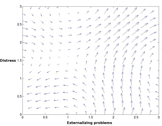
To illustrate the behavior of the NOLIDS model, Figure 1 is presented. It is a phase portrait of the momentary change in Externalizing problems and Distress according to the es-timated NOLIDS model when Timidity= 1 (i.e. there is a tendency to a problem with regard to timidity). The ar-rows indicate the movement in time of Externalizing prob-lems and Distress. For instance, two attractor regions are seen, namely the upper right part of the figure, indicating a

Table 2. Parameter estimates for the NOLIDS model.

Parameter f b g i a h Estimated value 0.6 0.7 0.8 0.2 0.1 0.3

Figure 1. Phase portrait of the change in Externalizing problems and Distress according to the estimated NOLIDS model when Timidity=

1. The arrows indicate the movement in time.

region characterized by both large Externalizing problems and Distress, where the movement in time is towards in-creased problems and, second, an attractor region in the lower left part of the figure, where the movements in time is towards decreased Externalizing problems.

To concentrate on the most important part of the model, consider Equation (2):

d E

d t = −D(D − (0.6 + 0.2T))(D − 3) − 0.1E(E − (0.7 + 0.2T ))(E − 3)

The dominant feature of Equation (2) is that, when Distress and Externalizing problems are not small, Externalizing problems will tend to increase over time. When they are both small, Externalizing problems will decrease. When Timidity= 0, tipping points are Distress= 0.6 and Externalizing problems= 0.7 and when Timidity= 2, tip-ping points are Distress= 1 and Externalizing problems= 1.1. Hence, the problem gravitation hypothesis earlier de-scribed (Point 3 above) is supported with tipping points at surprisingly low levels of Externalizing problems. The strength of the problem gravitation is, however, not large, as indicated by the small estimated parameter value of a.

The NOLIDS model’s fit to data was studied by generat-ing predictions of Externalizgenerat-ing problems at age 13 from the start values in the three adjustment problems at age 10 and then computing the correlation between the predicted and actual values. This correlation was 0.58 (R2= 0.34). Hence, the predictive power is marginally higher than that of the simple regression model and almost identical to that

of the more elaborated regression model.

Discussion

The NOLIDS model we presented was rather well aligned to the DS theory behind the scientific problem under study and the model addressed most of the hypotheses that were formed of the developmental process of the adjustment problems under study. Further, the properties of the esti-mated model could be interpreted in theoretically mean-ingful ways. The fit to data of the model was modest, as measured by the correlation between actual and model-predicted externalizing problems at age 13. However, the prediction was at least as good as that that produced by any of two standard linear regression models, and if a more a more ambitious optimization procedure of the NOLIDS model had been performed the prediction would have im-proved further. A useful property of the NOLIDS model is that its affinity to the DS theory makes it easy to modify the model in ways that make theoretical sense and that are not just based on improving statistical model fit.

As pointed out in the introduction, the NOLIDS model we presented should only be regarded as an illustrative ex-ample, pointing to the possibilities offered by this type of approach, also in situations with only a small number of measurement occasions. Despite its nice properties, the estimated NOLIDS model should not be considered a real model of the phenomena in Casti’s sense, i.e. it may not be a model that contributes to our understanding of the devel-opment of boys’ problem behavior. There are three reasons

for this:

• A more elaborate theoretical background than pre-sented here would be necessary to more fully reflect key theoretical conceptualization and to allow for a more precise specification of the model.

• The model construction and optimization of the esti-mated model parameters were done rather simplisti-cally.

• The information content of the data set was insuffi-cient for more stringent tests of model fit.

Consider now the NOLIDS model and the MRA Model (1) with regard to the criteria for a good model that were pre-viously described. In many criteria, the NOLIDS model stands out as the best one, especially with regard to

• criterion (1), the degree to which the model mirrors the theory

• criterion (4), the model allows for predictions outside the observed data space

• criterion (6), the explanatory power of the model Only in criterion (7), the simplicity of the model, the linear model is preferable because of its simple structure and that it contains only four parameters, as compared to six param-eters in the NOLIDS model. It should be pointed out that when we replaced our simple MRA model with a more elab-orated regression model that included nonlinear terms, the results of this comparison were only marginally changed; the major change being that the simplicity advantage of the linear model was lost.

There are a number of ways a NOLIDS model could be further developed. First, consider criterion (2) of a good model, i.e. how well the model fits to data. How “fit” should be best measured is far from a simple question. For instance, standard methods for measuring fit within the structural equation modeling tradition have limitations in that many fit measures are based on the similarity between the predicted and actual variance-covariance matrix, i.e. not based on the similarity between predicted and actual data. Given start values, a NOLIDS model can estimate val-ues simultaneously in all variables before and after the time point of the start values. This means that, if the data set is rich, a very stringent test of model fit can be achieved by comparing all these predicted values to actual values. A measure of concordance can be computed and a correla-tion coefficient is then an obvious candidate, although, de-pending on the context, better alternatives can be found. For an example of a more sophisticated method of mea-suring model fit, often used in chemistry, the reader is re-ferred toEdsberg(1991). However, maximizing a model’s fit to a data set is normally a complex, nonlinear optimiza-tion problem, and there is no guarantee the best soluoptimiza-tion is found (Nash & Sofer,1996). A special problem occurs when model fit is to be compared between a standard lin-ear regression model and a NOLIDS model. A crude “solu-tion” is then to ignore the NOLIDS models ability to predict all variables simultaneously and, as we did in this article,

just predict the outcome values in a single variable to ob-tain a comparison between predicted and actual values that conforms to what the linear model produces.

A NOLIDS model can be improved by introducing stochastic components that takes into account measure-ment errors and stochastic developmeasure-ment of the variables, like in models used for weather prediction. Such a model tends to be complicated and was not used in this article. This clearly is a limitation of our type of model, consider-ing that substantive errors of measurement are present in most areas in psychology. However, it is not a problem for the data we analyzed because the reliabilities of the teach-ers’ ratings can be assumed to be very high (certainly above 0.90). Using NOLIDS in future studies in contexts similar to ours but where the reliabilities of the involved variables are in the normal range (say, 0.60− 0.80) would make it necessary to use a model that can handle errors of measure-ment.

As was previously pointed out, NOLIDS models are com-ing into use in psychology but then mostly in experimen-tal contexts with very many measurement occasions and less frequently within a DS context. We believe our article has contributed to pointing out the possibility of using such models also in contexts when data only from a few mea-surement occasions are available (see also Boker, 2002). However, considering NOLIDS models potential to better match fundamental theoretical conceptualizations within DS, it is surprising that they are not more used in a DS context. Of course, many problems arise in the implemen-tation of such models. The technique is difficult and for long-term developmental studies a critical issue is the pos-sible lack of system invariance over the time period studied. In such studies the researcher might have to consider partly different systems operating during different time periods. If individual development is at focus, it can also be neces-sary to construct (partly) different models for different in-dividuals. In the present example, data from only two time points were used and with a three-year gap between mea-surements. This is, of course, sub optimal in that possible “nonlinear” movements of system states during these three years are lost and in that the data contain less rich infor-mation, decreasing the power of rejecting a “false” model.

We end with a strong plea made long ago by Aage Sörensen, an eminent sociologist:

The failure to consider mechanisms of change and try to formulate them in models of the processes we inves-tigate, however primitive the results may be, has im-portant consequences for the state of sociological re-search. The almost universal use of statistical models and specifications has two sets of important implica-tions. First, we are constrained by the statistical meth-ods to not consider whether or not we actually obtain, from our research, a greater understanding of the pro-cesses we investigate. In other words, the statistical models give us theoretical blinders. . . . Second, we may actually produce results that, on closer consideration, seem theoretically unfounded and very likely mislead-ing. (Sörensen,1998, pp. 14–15).

References

Bergman, L. R., & Andersson, H. (2010). The person and the variable in developmental psychology. Journal of

Psychol-ogy, 218, 155–165.

Bergman, L. R., & Magnusson, D. (1997). A person-oriented ap-proach in research on developmental psychopathology.

De-velopmental Psychopathology, 9(2), 291–319.

Bergman, L. R., & Vargha, A. (2012). Matching method to prob-lem: A developmental science perspective. European

Jour-nal of Developmental Psychology, 10(1), 9–28.

Boker, S. M. (2002). Consequences of continuity: The hunt for intrinsic properties within parameters of dynamics in psy-chological processes. Multivariate Behavioral Research(37), 405–422.

Boyce, W. E., & DiPrima, R. C. (1997). Elementary differential

equations and boundary value problems. New York: Wiley. Casti, J. L. (1989). Alternate realities: mathematical models of

nature and man. New York: Wiley.

Edsberg, L. (1991). Numerical experiments with parameter

estima-tion in systems of ordinary differential equaestima-tions(Tech. Rep. No. Trita-NA. 9101). Stockholm: KTH.

Granic, I., & Hollenstein, T. (2006). A survey of dynamic sys-tems methods for developmental psychopathology. In D. Ci-cchetti & D. J. Cohen (Eds.), Developmental psychopathology (2nd ed., Vol. 1: Theory and method, pp. 889–930). Hobo-ken, NJ, US: John Wiley & Sons Inc.

Grip, A. (2002). Linjära statistiska kontra ickelinjära dynamiska

modeller av individuell utveckling/linear statistical versus nonlinear dynamic models of individual development/

(Rap-porter från IDA projektet No. 81). Stockholms Universitet, Psykologiska Institutionen.

Kelso, J. A. S. (2000). Principles of dynamic pattern formation and change for a science of human behaviour. In L. R. Bergman, R. B. Cairns, L.-G. Nilsson, & L. Nystedt (Eds.),

Developmen-tal science and the holistic approach(pp. 63–83). Mahwah, New Jersey.

Magnusson, D. (1988). Individual development from an

interac-tional perspective: A longitudinal study. Hillsdale, NJ: Erl-baum.

Molenaar, P. C. M. (2004). A manifesto on psychology as id-iographic science: Bringing the person back into scien-tific psychology, this time forever. Measurement:

Interdis-ciplinary Research and Perspectives, 2, 201–218.

Nash, S. G., & Sofer, A. (1996). Linear and nonlinear

program-ming. Singapore. New York: McGraw Hill.

Needham, P. (2001). Law and order: Problems of empiricism in the

philosophy of science.(Lecture Notes in Philosophy, Vol. 4) Nesselroade, J. R., & Ram, N. (2004). Studying intraindividual

variability: What we have learned that will help us under-stand lives in context. Research in Human Development, 1, 9–29.

Peterson, D., & Eberlein, R. L. (1994). Reality check: a bridge between systems thinking and system dynamics. System

Dynamics Review, 2–3, 159–174.

Sörensen, A. (1998). Statistical models and mechanisms of social

processes.(Paper presented at the conference on Statistical Issues in the Social Sciences. Royal Swedish Academy of Sciences, Stockholm, Sweden)