Report number: 2009:38 ISSN: 2000-0456 Available at www.stralsakerhetsmyndigheten.se
Research and Development Program
in Reactor Diagnostics and Monitoring
with Neutron Noise Methods,
Stages 14 and 15
Research
Authors: Imre Pázsit Gustav Wihlstrand Tatiana Tambouratzis Anders Jonsson Berit Dahl
Title: Research and Development Program in Reactor Diagnostics and Monitoring with Neutron Noise Methods, Stages 14 and 15.
Report number: 2009:38.
Authors: Imre Pázsit, Gustav Wihlstrand, Tatiana Tambouratzis, Anders Jonsson and Berit Dahl. Chalmers University of Technology, Department of Nuclear Engineering, SE-412 96 Göteborg Date: December 2009.
This report concerns a study which has been conducted for the Swedish Radiation Safety Authority, SSM. The conclusions and viewpoints presented in the report are those of the author/authors and do not necessarily coin-cide with those of the SSM.
SSM Perspective Background
This report constitutes Stages 14 and 15 of a long-term research and deve-lopment program concerning the devedeve-lopment of diagnostics and moni-toring methods for nuclear reactors. Stage 14 was a full one-year project, whereas Stage 15 consisted of a half-year project.
Results up to Stage 13 were reported in SKI reports, as listed below and in the Summary. The results have also been published in international journals and have been included in both licentiate- and doctor’s degrees.
Objectives of the project
The objective of the research program is to contribute to the strategic research goal of competence and research capacity by building up compe-tence within the Department of Nuclear Engineering at Chalmers Univer-sity of Technology regarding reactor physics, reactor dynamics and noise diagnostics. The purpose is also to contribute to the research goal of giving a basis for SSM’s supervision by developing methods for identification and localization of perturbations in reactor cores.
Results
The program executed in Stages 14 and 15 consists of the following three parts:
• Study of criticality, neutron kinetics and neutron noise in molten salt reactors (MSR) (Stages 14 and 15);
• An overview and introduction to fuzzy logics (Stage 14), and an application to two-phase flow identification (Stage 15)
• Preparations for and execution of an IAEA-ICTP workshop on ”Neutron fluctuations, reactor noise and their applications in nuclear reactors” (Stage 14).
Project information
Responsible at SSM has been Ninos Garis. SKI reference: SKI 2007/1849-200705019 SSM reference: SSM 2008/3214
Previous SKI reports: 95:14 (1995), 96:50 (1996), 97:31 (1997),
98:25 (1998), 99:33 (1999), 00:28 (2000), 01:27 (2001), 2003:08 (2003), 2003:30 (2003), 2004:57 (2004), 2006:34 (2006), 2008:39
Contents
Contents ... 1
Summary ... 3
Sammanfattning ... 6
1 Study of neutron kinetics, dynamics and neutron noise in molten salt reactors (MSR) ... 9
1.1 Introduction ... 9
1.2 The empirical transfer function ... 10
1.3 Definition of the noise source and calculation of the induced noise in the point kinetic approximation ... 13
1.4 Neutron flux fluctuations for different fuel velocity and flux profiles ... 15
1.5 Space- time-dependent equations ... 19
1.6 Numerical solution ... 21
1.7 The Green’s function for infinite fuel velocity ... 24
1.8 Quantitative analysis ... 27
1.9 Conclusions ... 29
2 An overview of and introduction to fuzzy logic, and an application to two-phase flow identification ... 30
2.1 General description of the fuzzy logic method ... 30
2.2 A fuzzy inference system for identification of two-phase flow... 40
2.2.1 Introduction ... 40
2.2.2 Two-phase Flow Regime ... 42
2.2.3 Data ... 43
2.2.4 Flow Regime Identification via Sugeno-type FIS’s ... 44
2.2.5 Conclusions ... 45
3 Preparations for and execution of an IAEA-ICTP workshop on ”Neutron fluctuations, reactor noise and their applications in nuclear reactors ... 46
3.1 General description ... 46
Plans for the continuation ... 49
Acknowledgement ... 49
References ... 49
1 (68)
2 (68)
Summary
This report gives an account of the work performed by the Department of Nuclear Engineering, Chalmers University of Technology, in the frame of a research contract with the Swedish Nuclear Power Inspectorate (SKI), contract Nos. SSM 2008/180 and SSM 2008/3214. The present report is based on work performed by Imre Pázsit, Gustav Wihlstrand, Tatiana Tambouratzis, Anders Jonsson and Berit Dahl, with Imre Pázsit being the project leader.
This report describes the results obtained during Stages 14 and 15 of a long-term research and development program concerning the development of diagnostics and monitoring methods for nuclear reactors. The long-term goals are elaborated in more detail in e.g. the Final Reports of stage 1 and 2 (SKI Report 95:14 and 96:50, Pázsit et al. 1995, 1996). Results up to stage 13 were reported in (Pázsit et al. 1995, 1996, 1997, 1998, 1999, 2000, 2001, 2003, 2004; Demazière et al, 2004; Sunde et al, 2006: Pázsit et al. 2008). A brief proposal for the continuation of this program in Stage 16 is also given at the end of the report.
The program executed in Stages 14 and 15 consists of three parts and the work performed in each part is summarized below.
1. Study of neutron kinetics, dynamics and neutron noise in molten salt reactors (MSR)
In the previous report, Stage 13, a simple one-dimensional model with propagating fuel properties was set up and studied as a model of a molten salt reactor. The solution of the static eigenvalue equation was given first by expansions into eigenfunctions of a corresponding traditional reactor, i.e. an MSR with fuel velocity . As one step towards the calculations of the noise in the point kinetic approximation, a simplified empirical model of the zero reactor transfer function , suggested in the literature, was investigated. It was noticed that both the static flux as well as the transfer function were rather similar to their counterparts, hence it appeared that the calculation of the noise, induced by propagating perturbations, will be rather simple in the point kinetic approximation, and can be based on results and methods of traditional reactors. Obviously, this means that the results would not show much difference from the noise induced in a traditional system either, at least what regards the point kinetic approximation.
0
u =
0( )
G ω
In Stage 14 we first investigated the empirical zero power transfer function of an MSR more closely, and found that it shows some small irregularities, which are related to the transport time of the fuel in the external loop from the core exit to core inlet. Then we turned to the calculation of the point kinetic noise, induced by propagating perturbations. The point kinetic noise induced by propagating perturbations was investigated in the past, and it is known that this approximation predicts a periodic sequence of peaks and sinks in the frequency domain, arising from the properties of the perturbation. We extended this model by assuming several fuel channels radially, with different velocities. It was shown, with the use of the traditional zero power transfer function, that in case of
3 (68)
different fuel velocities in the core (the existence of a radial velocity profile), the sink structure of the induced noise becomes shallower.
In Stage 15, the solution of the space-dependent noise problem was started with the calculation of the Green’s function of the problem. It turned out that the same technique of eigenfunction expansion that was used in the static eigenvalue problem, does not work, because of the singularity of the solution at the perturbation point (discontinuous derivative). The solution showed non-physical spatial oscillations, hence only the frequency dependence could be investigated. This showed that the solution obtained from the space-dependent equations, which is free from the phenomenological simplifications that are used in the empirical transfer function, had much larger and narrower peaks at the inverse of the total recirculation time of the fuel. Hence the validity of the empirical transfer function, used in the literature, is limited.
The space-dependent problem was solved for the case of infinite fuel velocity, with a new technique with separates out a singular and a non-singular term in the solution, similarly to the method of eliminating the uncollided flux in transport problems. A closed analytical solution was obtained for the Green’s function. The technique can also be applied with finite fuel velocity, eliminating the singular term from the eigenfunction expansion, which will then converge much faster. A quantitative study of the solution showed, in a comparison with a traditional system of similar parameters, that the noise amplitude is much higher in an MSR for low and intermediate frequencies, and that the point kinetic behaviour exists for higher frequencies or system sizes than in a traditional reactor.
2. An overview of and introduction to fuzzy logics, and an application to two-phase flow identification
The purpose of Stage 14 was to get acquainted with the methodology of fuzzy logic techniques, and give an overview and introduction, since this technique is new to us. Fuzzy logic (FL) constitutes a soft computing methodology that supports computing with words rather than with numbers; although words are inherently less precise than numbers, manipulating the former exploits the tolerance for imprecision and, thus, lowers the computational cost while also increasing robustness. FL supports both data processing (by allowing varying degrees of membership rather than crisp set membership/non-membership to overlapping sets) and inference-making (by manipulating if-then rules, where both consequent and antecedent variables are expressed via FL). By incorporating simple if-then rules between FL variables, fuzzy inference systems (FS’s) solve prediction and control problems without the need to mathematically model the underlying problem structure.
In Stage 15 the method was applied to a problem which was already tackled by us by other types of soft computing methods, namely identification of two-phase flow regimes by artificial neural networks. This time the flow regime identification was attempted by fuzzy logics methods. An efficient, on-line, non-invasive FS was put forward for identifying the two-phase flow regime that occurs in the coolant pipes of boiling water reactors (BWRs). The frames of the dynamic neutron radiography video collected at the Kyoto University Research Reactor Institute (KURRI) and recording four principal flow regimes (bubbly, slug, churn and annular) were used. A single FS input (the mean image
4 (68)
intensity, giving a measure of bubble quantity in the frame) was employed. The FS comprises four fuzzy inference rules (one per flow regime) and a single output expressing the predicted flow regime. Five-fold cross-validation testing of the FL demonstrated superior performance to that of previous on-line approaches in terms of both efficiency and accuracy.
3. Preparations for and execution of an IAEA-ICTP workshop on ”Neutron fluctuations, reactor noise and their applications in nuclear reactors”
The Workshop was held according to the plans between 22-26 September 2008 at the premises of the International Centre for Theoretical Physics, Trieste. Our Department was the main organizer and three members (Imre Pázsit, Christhope Demazière and Andreas Enqvist) gave 80% of all the lectures.
The course included the theory and application of both zero power noise and power reactor noise methods. For these two main subjects we produced one lecture note for each. A special part of the course concerned transport in stochastic media, with applications to advanced reactors with stochastic composition, such as the pebble bed reactor, or reactors run on MOX fuel. Some lectures were devoted to experimental methods and the analysis of measurements from research reactors and power plants. At the end of the course the participants received written test questions. The workshop was attended by about 30 participants.
5 (68)
Sammanfattning
Denna rapport redovisar det arbete som utförts inom ramen för ett forskningskontrakt mellan Avdelningen för Nukleär Teknik, Chalmers tekniska högskola, och Statens Kärn-kraftinspektion (SKI), kontrakt Nr. SSM 2008/180 och SSM 2008/3214. Rapporten är baserad på arbetsinsatser av Imre Pázsit, Gustav Wihlstrand, Tatiana Tambouratzis, Anders Jonsson och Berit Dahl, med Imre Pázsit som projektledare.
Rapporten beskriver de resultat som erhållits i etapp 14 och 15 av ett långsiktigt forsknings- och utvecklingsprogram angående utveckling av diagnostik och övervakningsmetoder för kärnkraftsreaktorer. De långsiktiga målen har utarbetats noggrannare i slutrapporterna för etapp 1 och 2 (SKI Rapport 95:14 och 96:50, Pázsit et al. 1995, 1996). Uppnådda resultat fram till och med etapp 13 har redovisats i referenserna (Pázsit et al. 1995, 1996, 1997, 1998, 1999, 2000, 2001, 2003, 2004;. Demazière et al, 2004; Sunde et al, 2006; och Pázsit et al, 2008). Ett kortfattat förslag till fortsättning av programmet i etapp 16 redovisas i slutet av rapporten.
Det utförda forskningsarbetet i etapp 14 och 15 består av tre olika delar och arbetet i varje del sammanfattas nedan.
1. Studier av kriticitet, neutronkinetik och neutronbrus i reaktorer med flytande bränsle (saltsmältereaktorer, molten salt reactors, MSR)
I den tidigare rapporten, etapp 13, byggdes en enkel, endimensionell modell med rörligt bränsle upp och studerades som en modell av en saltsmältereaktor. Lösningen till den statiska egenvärdesekvationen gavs först som utvecklingar i egenfunktioner till en mot-svarande traditionell reaktor, dvs. en MSR med bränslehastighet . En förenklad, empirisk modell av överföringsfunktionen för nolleffektsreaktorn, , undersöktes som ett steg mot beräkningar av bruset i den punktkinetiska approximationen, enligt ett förslag i litteraturen. Både det statiska flödet och överföringsfunktionen visade sig vara ganska lika sina traditionella motsvarigheter. Det verkade därför som om beräkningen av bruset som orsakas av propagerande störningar skulle kunna baseras på resultat och metoder från traditionella reaktorer. Detta skulle självklart innebära att inte heller resultatet skulle skilja sig alltför mycket från bruset i ett traditionellt system, åtminstone vad beträffar den punktkinetiska approximationen.
0
u =
0(
G ω)
I etapp 14 undersökte vi först noggrannare den empiriska överföringsfunktionen för nolleffektsreaktorn hos en MSR. Vi fann att den visar några små oregelbundenheter, som har med bränslets transporttid i den externa loopen från härdens utlopp till dess in-lopp att göra. Sedan angrep vi problemet med att beräkna det punktkinetiska brus orsakat av propagerande. Detta brus undersöktes tidigare och det är känt att denna approximation förutspår en periodisk sekvens av toppar och sänkor i frekvensområdet pga. störningens egenskaper. Vi utökade denna modell genom att anta flera radiella bränslekanaler med olika hastigheter. Genom att använda den traditionella överföringsfunktionen från nolleffektsreaktorn kunde vi visa att strukturen hos det inducerade brusets sänkor blir grundare med olika bränslehastigheter i härden, (dvs. när det finns en radiell hastighetsprofil).
6 (68)
I etapp 15, började vi lösa det rumsberoende brusproblemet med att beräkna Greens funktion för problemet. Det visade sig att den teknik med utveckling i egenfunktionerna, som användes i det statiska egenvärdesproblemet, inte fungerade pga. lösningens singularitet i störningspunkten (diskontinuerlig derivata). Lösningen uppvisade ickefysikaliska oscillationer i rummet. Följaktligen kunde endast frekvensberoendet undersökas. Detta visade att lösningen som erhölls från de rumsberoende ekvationerna, som är befriade från de fenomenologiska förenklingar som används i den empiriska överföringsfunktionen, hade mycket högre och smalare toppar vid inversen av den totala omloppstiden för bränslet. Följaktligen är giltigheten hos den empiriska överföringsfunktion, som används i litteraturen, begränsad.
Det rumsberoende problemet löstes i fallet med oändlig bränslehastighet med en ny metod som delar upp lösningen i en singulär och en icke-singulär term, liknande metoden att eliminera det okolliderade flödet i transportproblem. En sluten analytisk lösning erhölls för Greens funktion. Tekniken kan också användas för ändlig bränsle-hastighet, då den singulära termen försvinner från egenfunktionsutvecklingen, och lösningen konvergerar mycket snabbare. En kvantitativ undersökning av lösningen vi-sade att brusamplituden för låga och medelhöga frekvenser är mycket högre i en MSR jämfört med ett traditionellt system med likartade parametrar. Det punktkinetiska uppförandet existerar för högre frekvenser eller systemstorlekar jämfört med en traditio-nell reaktor.
2. En översikt av och introduktion till fuzzy logic och en tillämpning på identifika-tion av tvåfasflöde.
Målet med etapp 14 var att bekanta oss med fuzzy logic-metodiken och ge en översikt och introduktion, eftersom denna metod är ny för oss. Fuzzy logic (FL) är en så-kallad ”soft computing method” (”mjuk algorithm”), som stödjer databehandling med ord snarare än siffror. Även om ord till sin natur är mindre precisa än tal, så möjliggör just detta att manipulationen blir mindre känsligt för osäkerheter, vilket leder till både lägre beräkningsinsatser och större robusthet.
FL stödjer både databehandling (genom att tillåta varierande grad av medlemskap sna-rare än en bestämd uppsättning medlemmar eller icke medlemmar) och slutledning (genom att använda ”if-then”-regler, där både efterföljande och föregående variabler ut-trycks genom FL). Diffusa (Fuzzy) slutledningssystem (FS) löser problem rörande förutsägelser och kontroll utan att matematiskt behöva modellera den underliggande problemstrukturen genom att infoga enkla ”if-then”-regler mellan FL-variabler.
I etapp 15 användes metoden på ett problem som vi redan tidigare angripit med andra mjukvarumetoder, nämligen att identifiera tvåfasflödesområden med hjälp av artificiella neurala nätverk. Nu försökte vi använda FL-metoder för flödesområdesidentifikationen. En effektiv, on-line,, icke-störande FS ställdes upp för att identifiera tvåfasflödesregimer i kylvattenrören hos kokvattenreaktorer (BWRs). Dynamiska neutronradiografibilder (frames) på videoupptagningar från Kyoto University Research Reactor Institute (KURRI) och inspelning av de fyra väsentligaste flödesregimerna (bubbly, slug, churn och annular) användes. En enda indatamängd (medelintensiteten i bilden , som ger ett värde på andelen bubblor på bilden) till FS användes. FS inkluderar fyra diffusa slutsatsregler (en per flödesregim) och ett enda utdatavärde som bestämmer
7 (68)
flödesregimen. Femfaldig korsvalidering av FL visade överlägsen prestanda jämfört med tidigare on-line behandlingssätt, både vad gäller effektivitet och exakthet.
3. Förberedelser till, och genomförandet av IAEA-ICTP workshopen ”Neutron fluctuations, reactor noise and their applications in nuclear reactors”
Denna workshop hölls planenligt den 22 - 26 september 2008 på International Centre for Theoretical Physics i Trieste. Vår avdelning var huvudorganisatör och tre av våra medlemmar (Imre Pázsit, Christhope Demaizère och Andreas Enqvist) höll 80% av alla föreläsningar.
Kursen behandlade teori och tillämpning av både nolleffektbrus och metoder för brus i effektreaktorer. Vi skrev föreläsningsanteckningar till vardera av dessa två huvudämnen. En speciell del av kursen rörde transport i stokastiska media med tillämpningar inom avancerade reaktorer med slumpmässig sammansättning, såsom kulbäddsreaktorn eller reaktorer som använder MOX-bränsle. Några föreläsningar rörde experimentella meto-der och analys av mätningar från forskningsreaktorer och kärnkraftverk. På slutet av kursen fick deltagarna skrivna testfrågor. Cirka 30 personer deltog i workshopen.
8 (68)
1 Study of neutron kinetics, dynamics and neutron
noise in molten salt reactors (MSR)
1.1 Introduction
In the previous report, Stage 13, a simple one-dimensional model with propagating fuel properties was set up and studied as a model of a molten salt reactor. The solution of the static eigenvalue equation was given first by expansions into eigenfunctions of a corresponding traditional reactor, i.e. an MSR with fuel velocity . In preparations for the calculations of the noise in the point kinetic approximation, a simplified empirical model of the zero reactor transfer function , suggested by MacPhee (1958) and used by Dulla (2005), was investigated. It was noticed that both the static flux as well as the transfer function were rather similar to their counterparts, hence it appeared that the calculation of the noise, induced by propagating perturbations, will be rather simple in the point kinetic approximation, and would not show much difference from the noise induced in an traditional system. The noise in the point kinetic approximation was studied in systems with propagating perturbations in the past, and it is known that this approximation predicts a periodic sequence of peaks and sinks in the frequency domain, arising from the properties of the perturbation.
0
u =
0( )
G ω
The goal in Stage 14 was therefore to perform a quantitative analysis of the noise in the point kinetic approximation, with an extension to the case when there are several channels with different velocities, to see how the co-existence of several velocities distorts the known sink structure. At the same time we noted that the empirical model of the for MSR contains some ripples which were not noted in the previous Stage. These are related to the recirculation time of the fuel, and to the transit time of the fuel in the core. The work in Stage 14 consists of both a quantitative analysis of the fine structure of the zero power reactor transfer function for MSR, and the frequency dependence of the noise induced by propagating perturbations in the point kinetic approximation. Several cases with different radial velocity distributions were investigated quantitatively.
0( )
G ω
In Stage 15 we turned to the solution of the space-dependent equations. A first idea was a rigorous derivation of the point kinetic approximation with the Henry factorisation procedure, but this was postponed because it requires the knowledge of the adjoint function. It turns out that the one-group diffusion equations for an MSR are not self-adjoint, due to the directed flow of the fuel. Hence for the MSR a method has to be found to define the adjoint, and this was postponed to the next Stage. The space-dependent equations were then solved for the Green’s function of the system by the same eigenfunction expansion technique as in the static case. It turned out, however, that due to the discontinuity of the Green’s function at the point of the perturbation, the solution for the noise equations with this method is much more complicated than in the static case. The quantitative results showed that the space dependence of the induced noise was not reliably reconstructed by the method, because of the need of very many
9 (68)
terms to satisfy the discontinuity. The frequency dependence, on the other hand, was reliably reconstructed.
In Stage 15 therefore two paths were followed. Partly, the frequency dependence of the space-dependent Green’s function was investigated in a few spatial points. A comparison with the empirical suggestion for the showed that for cases where the space-dependent solution is expected to behave in a point kinetic way, i.e. for small reactors at low frequencies, the two solutions still differ significantly. This indicates the insufficiency of the empirical model.
0( )
G ω
The other path was to calculate the Green’s function for infinite fuel velocity. For such a case, a compact analytical solution can be found with a method which is similar to the elimination of the uncollided flux in transport problems. The significance and use of such a solution arises from the fact that the case of infinite velocity can be considered as the maximum deviation from the traditional reactors in some sense, thinking of the fact that the of an MSR with all material and geometrical parameters constant behaves monotonically as a function of the fuel velocity. Hence the behaviour of the system as a function of system size and perturbation frequency can be studied and compared with traditional systems. The comparison showed that an MSR behaves point kinetically for higher frequencies or system sizes than a traditional reactor of equivalent parameters.
eff
k
1.2 The empirical transfer function
We first re-capitulate the basic properties of the model used in Stage 13, which will also be used here. A one-dimensional model will be used, where the spatial dimension is along the z axis, and the fuel is propagating in the core with a velocity u in this direction. The core boundaries are located between and z . The outlet of the core is connected back to the inlet with an external loop of length L, hence the total recirculation path of the fuel is T H .
0 z = L H = = +
In Stage 13, the empirical model of the zero power transfer function from Dulla (2005) was introduced. This transfer function is obtained from the modified point kinetic equations, which model the recirculation properties of the delayed neutron precursors: 0( ) G ω ( ) ( ) ( ) ( ) fluid t dP t P t C t dt δρ ρ β λ + − = Λ + (1) and ( ) ( ) ( ) ( ) ( ) l l c c dC t C t C t e P t C t dt λτ β λ τ τ − − = − − + Λ τ (2)
Here, the parameters and are the transit time of the fuel in the
core and in the external loop of length L, respectively. If the steady state condition is imposed, the value of
/ c H u τ = τ =l L u/ fluid ρ ) l τ −
can be calculated. Setting the time derivatives and to zero, and C t that must hold in steady state operation, one obtains
( )t δρ
( )=C t(
10 (68)
1 (1 exp{ }) (1 exp{ }) R i i fluid i i c i l β λ τ ρ λ τ λ τ = − − = + − −
∑
l (3)With the above, the transfer function becomes 0 1 ( ) 1 exp{ ( )} fluid l c G i i i ω λβ ω ρ β τ λ ω ω λ τ = Λ − + − − − + + + (4)
This can be compared with the transfer function for traditional reactors, which reads as 0 1 ( ) ( ) G i i ω β ω ω λ = Λ + + (5)
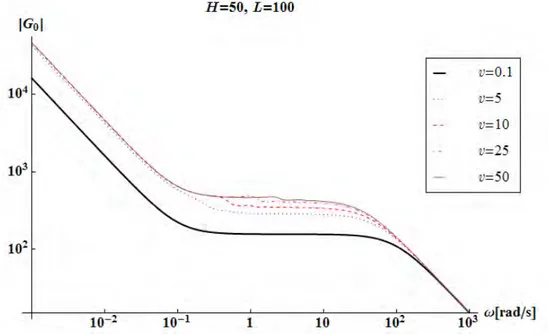
On the first sight, the structure of Eq. (4) does not seem to change much when different values of τ and are used, as illustrated in Fig. 1. The similarity of the empirical MSR transfer function and that of the traditional case, Eq.
c τl
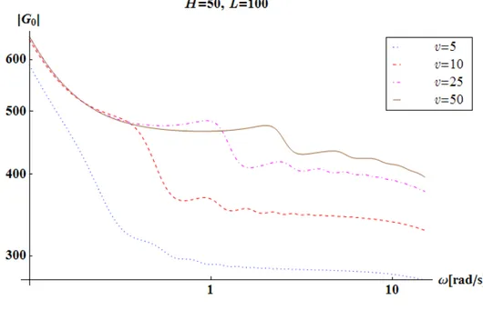
(5), was noted in Stage 13. However, a closer look reveals in Fig. 1 small ripples in the curves for the larger fuel velocities. For the lowest velocity, v = 0.1 cm/s, the curve seems completely smooth. The irregularities are more obvious if we enlarge the interesting region, Fig. 2.
Fig. 1. The transfer function for different values of the fuel velocity, vin cm/s.
11 (68)
Fig. 2. Enlarged plot of irregularity region of the transfer function. Velocity v in cm/s.
From this figure one can see that the starting frequency, as well as the frequency separation of the peaks increases with increasing fuel velocity (note the logarithmic scale on the x-axis). The peaks can be approximately evaluated/identified manually from Mathematica plots and the distance between the peaks can thus be determined. It is seen that the distances between the peaks are approximately equal for each velocity and that the peak distances increase with increasing fuel velocity. It is easy to confirm, which can also be expected from Eq. (2), that these are related to the frequency corresponding to the transition time in the external loop,
2 l l π ω τ = (6)
The peak distances for different values of v, H and L, denoted as and determined from the plots, correspond to . This is illustrated in Fig. 3. We will return to these small peaks below in connection with the solution of the space-dependent problem.
diff ω l ω 12 (68) SSM 2009:38
0.62 diff
ω =
Fig. 3. Behavior for different values of H and L at a velocity v = 10 cm/s
, ωL =0.63 ωdiff =0.31, ωL =0.31 ωdiff =0.21, ωL = 0.21
0.63 diff
ω = , ωL =0.63 ωdiff =0.32, ωL =0.31 ωdiff =0.21, ωL = 0.21
1.3 Definition of the noise source and calculation of the induced noise
in the point kinetic approximation
In the simple one-group model used here, the reactivity induced by the fluctuations of the absorption cross section are given in first order perturbation theory as
2 0 2 0 ( , ) ( ) ( ) ( ) a f r t r dr t r dr δ φ ρ ν φ Σ = − Σ
∫
∫
(7)Because we will consider a horizontal velocity profile of the fuel in the core and hence conceptual second dimension, we kept the more general notation on the spatial co-ordinates. Eq. (7) can be brought into a simpler form by introducing the normalized flux: (8) 0( )r c ( )r φ = ⋅ϕ0 with: 2 0( ) c =
∫
φ r dr (9) so that: 2 0( )r dr 1 ϕ =∫
(10)Using the relations above, the reactivity (7) becomes:
13 (68)
2 0 1 ( ) ( ) a( , ) f t r ρ ϕ δ ν = − Σ Σ
∫
r t dr (11)and in the frequency domain:
2 0 1 ( ) ( ) a( , ) f r r d ρ ω ϕ δ ω ν = − Σ Σ
∫
r (12)The perturbation in Eq. (11), which propagates in the z direction, can be written as:
( , ) ( 0, ) a a z z t z t u δΣ = Σδ = − (13)
In the frequency domain this yields
( , ) (0, ) exp{ } exp{ } a z a i z k u u ω δΣ ω = Σδ ω ⋅ ∼ i ωz ω (14) where it was assumed that the fluctuations at the inlet, , constitute a white
noise process with a constant power spectrum. Hence, the reactivity effect of the perturbation is: (0, ) a δΣ 2 0 0 ( ) ( )exp{ } H f k z i z u ω ρ ω ϕ ν = − Σ
∫
dz ] (15) In an MSR, the fuel flows in several parallel channels, such that the vertical velocitydepends on the radial position of the channel. This effect will be simulated here by assuming a radial extension of the reactor along the x axis, with the extent of the core being between [ . If the fuel velocity has a profile , i.e. if it varies radially, then Eq. , a a − u =u x( ) (15) becomes: 2 2 0 0 0 ( ) ( ) ( )exp{ } ( ) H a f a k z x i z dxdz u x ω ρ ω ϕ ϕ ν − = − Σ
∫ ∫
(16)where it was assumed that because of the simple geometry of the reactor, the static flux is factorised: 0 0 0 1 2 ( ) ( ) ( ) cos sin 2 x r x z a H H a π ϕ =ϕ ϕ = ⎜⎛⎜⎜⎜ ⎟⎟⎟⎟⎞ ⎛⎜ ⎝ ⎠ ⎝ z π ⎞⎟ ⎜ ⎟ ⎜ ⎟ ⎜ ⎟⎠ t (17) In the calculations, we shall assume both a radially varying profile as in (17) above, and
a flat flux profile, ϕ0( )x =cons .
The neutron noise in the point kinetic approximation can be written as:
(18)
0 0
( , )r ( ) ( ) ( )r G δφ ω =φ ω ρ ω
As is known, in this approximation the space and the frequency dependence is factorised. In the forthcoming, the frequency dependence of this quantity will be investigated. Because of the similarity of the transfer function of the MSR and that of the traditional reactors, the latter simpler transfer function, Eq. (5) will be used here.
14 (68)
1.4 Neutron flux fluctuations for different fuel velocity and flux
profiles
We will calculate the neutron noise with either constant fuel velocity , or with a horizontal velocity profile along the direction x, which is perpendicular to z, in the form
0 u =u 0 ( ) cos( ) 2 ' x u x u a π = (19)
Here the parameter will be chosen as . For , the velocity is zero
at the reactor boundary; a value will describe a slowly changing velocity profile. The velocity profile of Eq.
' a a ≤a'≤ ∞ a ' a =a ' a
(19) is symmetric, and has a maximum in the centre of the core. If a is increased, the profile becomes flatter.
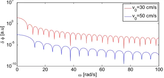
Starting with a constant fuel velocity profile, it is noticed that the frequency of the first sink increases with fuel velocity. The sinks occur at the frequencies (Pázsit, 2002):
2 ; 2, 3 n c c n n n π ω ω τ = = = … (20)
Two cases with different velocities are shown in Fig. 4. It is seen in the expressions for the reactivity that a higher fuel velocity (shorter core transit time) corresponds to higher sink frequencies, according to (20).
Fig. 4. Neutron flux fluctuations for two fuel velocities. A higher fuel velocity gives fewer sinks. 0 20 40 60 80 100 10-10 10-5 100 105 ω [rad/s] δ φ [a .u ] v0=30 cm/s v0=50 cm/s 15 (68) SSM 2009:38
0 5 10 15 20 v_0 radial distance [cm] fu el v el oc ity [c m /s ]
Fig. 5. A varying and a flatter fuel velocity profile.
Turning to the velocity profile, Eq. (19), in the numerical work a radial system half-width of cm will be used. Two different velocity profiles will be considered,
one with d one with cm. They are shown in Fig. 5.
20
a =
a'= =a 20cm, an a'=10a =200
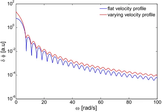
Using the more rapidly varying profile in Fig. 5 means that there are a larger number of different fuel velocities in the core. Each velocity will have different sink frequencies. Adding these up via the integral (16) will result in shallower sinks, as seen in Fig. 6.
0 20 40 60 80 100 10-6 10-4 10-2 100 102 ω [rad/s] δ φ [a .u ]
flat velocity profile varying velocity profile
Fig. 6. Neutron flux fluctuation for two fuel velocity profiles with u=30 cm/s. In the curve with deeper sinks the flatter velocity profile is used.
16 (68)
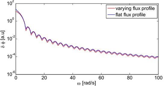
0 20 40 60 80 100 10-6 10-4 10-2 100 102 ω [rad/s] δ φ [a .u ]
varying flux profile flat flux profile
Fig. 7. Noise for two different combinations of flux- and fuel velocity profiles. In both plots a varying fuel velocity profile is used, but the plots have different flux profiles. It is seen that changing the flux profile has little effect on the sink structure
when the velocity profile is varying.
Comparing two cases where the velocity profile is strongly varying in both cases but the flux is flat in one case and varying in the other, a calculation of the neutron noise shows that the sink structure of the neutron noise does not change much. This is shown in Fig. 7.
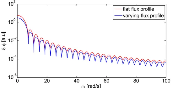
Comparing two noise plots, where both have flat fuel velocity-profile but different flux profiles, it is seen that the one with the flat flux-profile has more shallow sinks, as seen in Fig. 8.
17 (68)
Fig. 8. Noise for different combinations of flux-and fuel velocity profiles. In both plots a flat fuel velocity profile is being used, but the plot with deeper sinks
corresponds to a varying flux profile.
0 20 40 60 80 100 10-6 10-4 10-2 100 102 ω [rad/s] δ φ [ a .u ]
flat flux profile varying flux profile
One notices that changing the flux-profile does not significantly affect the sink structure much when the fuel velocity-profile is varying, compared to the situation when the fuel velocity-profile is flat.
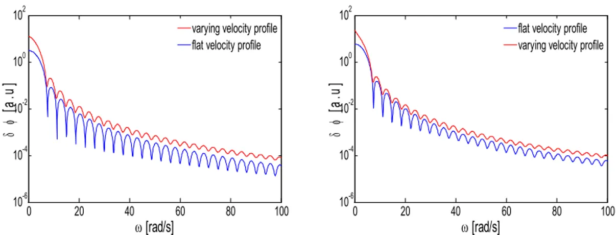
The same information is shown in Fig. 9, but in a different combination. On the left figure the flux profile is flat, whereas on the right figure it is varying. In both Figures two cases are shown, one with a flat velocity profile (deep sinks) and one with a varying velocity profile (shallower sinks). The difference between the deep and the shallow sinks is larger on the left figure, which belongs to the flat radial flux profile. The reason why the difference becomes smaller in the case of varying flux profile is that the effect of different velocities, leading to shallower sinks, is counteracted by the fact that the contribution from the different velocities is weighted by the flux shape, as shown in Eq. (16). In other words, if the flux profile is varying, the fuel velocities close to the edges of the reactor contribute less to the induced noise.
Some more details and cases can be found in Wihlstrand (2008).
18 (68)
Fig. 9. Noise when changing the velocity profile, keeping the same flux profile. It is seen that changing the velocity profile has a stronger effect on the sink structure of the neutron noise when the flux profile is flat (left), compared to the case of flux strongly
varying profile (right).
0 20 40 60 80 100 10-6 10-4 10-2 100 102 ω [rad/s] δ φ [a .u ]
varying velocity profile flat velocity profile
0 20 40 60 80 100 10-6 10-4 10-2 100 102 ω [rad/s] δ φ [a .u ]
flat velocity profile varying velocity profile
1.5 Space- time-dependent equations
We shall now calculate the space-dependent neutron noise. The starting equations are ( ) ( ) ( ) ( ) ( , 1 , f 1 a , z t D z t z t C z v t φ φ ν β φ λ ∂ ⎡ ⎤ = Δ + Σ⎣ − − Σ ⎦ + ∂ ,t (21) )
( )
,( )
,( )
(
, f C z t C z t u z t t z βν λ ∂ ∂ + = Σ − ∂ ∂ C z t,)
(22)Assume a critical system with Σ =a const and a time-dependent system with
( ), ( )
a z t a δ a z t
Σ = Σ + Σ
(
, . In this Stage we shall calculate the Green's function, where the structure of δΣa z t, ) is not important. Later we shall assume a propagating perturbation ( ), 0, a a z z t t u δΣ = Σδ ⎛⎜⎜⎝ − ⎟⎟⎟⎞⎠ ) , ) , H (23) in the core. Even later, we shall account for the fact that some of the perturbation which
leaves the core, may return in a damped form to the inlet and the effect of several cycles may pile up.
We use the usual assumptions of splitting the time-dependent quantities into a mean value and a fluctuating part:
(24) (z t, ) 0( )z (z t φ =φ +δφ and (25) ( , ) 0( ) ( C z t =C z +δC z t
The boundary conditions are
(26) (0,t) 0( )0 (H t, ) 0( ) 0
φ =φ =φ =φ =
19 (68)
(27) (0,t) (H t, ) 0
δφ =δφ =
for the static flux and the noise, and
(28) ( )0,
(
,)
l l C t =C H t−τ e−λτ and hence (29) (0, )(
,)
l l C t C H t e λτ δ =δ −τ −for the delayed neutron precursors. Neglecting second order terms and subtracting the static equations yields
( )
( )
(
)
(
(
)
)
( ) ( )
0 , 1 , 1 , , f a a z t D z t z v t z t z t z δφ δφ ν β δφ λδφ λ φ ∂ ⎡ ⎤ = Δ + Σ⎢⎣ − − Σ ⎥⎦ ∂ + − Σ ,t (30)( )
,( )
,( )
(
1 , f C z t C z t u z t v t z δ δ βν δφ λδ ∂ ∂ + = Σ − ∂ ∂ C z t,)
(31)After a temporal Fourier-transform, and some re-arrangement, one obtains that
( , ) f (1 ) a i ( , ) a( , ) 0( ) D z z z v ω δφ ω ⎡ν β ⎤δφ ω δ ω φ Δ + Σ⎢⎢ − − Σ − ⎥⎥ = Σ ⎣ ⎦ z (32)
( )
, C z( )
, f( )
,(
i C z u z C z z δ ω ωδ ω + ∂ =βν δφΣ ω −λδ ω ∂ ,)
(33)The boundary condition for δC z( ,ω) in the frequency domain reads as
( )
0,(
,)
(i )l(
,)
( )C C H e ω λ τ C H e λ ω τ
δ ω =δ ω − + =δ ω − l (34)
Following the solution for the static case for (33) as described in the previous Stage, one obtains a similar result with the only difference that one has to make the replacement
. We will use this condensed notation for simplicity. ( ) i λ → +λ ω ≡λ ω ( ) ( ) ( ') 0 ( , ) (0, ) ( ', ) ' z z f z z u u C z C e e z dz u λ ω βν λ ω δ ω =δ ω − + Σ
∫
− − δφ ω (35) Utilizing (34) in (35) gives ( ) ( ) ( ) ( ) ( ) 0 ( , ) (0, ) (0, ) , l c c H z f u C H C e C e e e z d u λ ω τ λ ω λ ω τ λ ω τ δ ω δ ω βν δ ω − − δφ ω = Σ = +∫
z (36)From here one obtains
( ) ( ) ( ) ( ) ( ) ( ) ( ) ( ) ( ) 0 0 (0, ) , , 1 c l c H z f u H z f u e C e u e e e e z dz u e λ ω λ ω τ λ ω τ λ ω τ λ ω λ ω τ λ ω τ βν δ ω δφ ω βν δφ ω − − − − Σ = − Σ = −
∫
∫
z dz (37) 20 (68) SSM 2009:38and hence ( ) ( ) ( ) ( ) ( ) ( ) ' 0 0 ( , ) , ( ', ) ' 1 H z z f z z u e u u C z e e z dz e z dz u e λ ω λ ω τ λ ω λ ω λ ω τ βν δ ω = − Σ ⎪⎨⎪⎧ − − δφ ω + δφ ω ⎫⎪⎪⎬ ⎪ − ⎪ ⎪ ⎪ ⎩
∫
∫
⎭ (38) Substituting this into (32), one obtains for the neutron noise the expression( ) ( ) ( ) ( ) ( )
( ) ( )
' 0 0 , ( , ) (1 ) ( , )( , )
( ', ) '
1
a z f u H z z z u u z z i D z f a z e v ue
e
z
dz
e
z
d
e
λ ω λ ω λ ω λ ω τ λ ω τ ω φ βν ω φ ω ν β δφ ω λδφ ω
δφ
ω
δ
− − − Σ Δ + Σ⎡⎢ − −Σ − ⎤⎥ + ⎢ ⎥ ⎣ ⎦ ⎧ ⎫ ⎪ ⎪ ⎪ ⎪ ⎪ ⎪ ⎨ ⎬ ⎪ ⎪ ⎪ ⎪ ⎪ ⎪ ⎩ ⎭+
−
= Σ
∫
∫
z
(39)The Green's function of this equation is defined by replacing the noise source on the r.h.s. with a Dirac-delta function, i.e.
( ) ( ) ( ) ( )
(
)
( ) ' ' 0 0 ( , ) (1 ) ( , ) , , , ,( ',
) '
( ',
) '
1
z u f p p p H z z z u u p p G G i D G z z f a G z z e v u z ze
e
z z
dz
e
z z
d
e
λ ω λ ω λ ω λ ω τ λ ω τ βν ω ω ν β ω λω
φ
δ
− − − Σ Δ + Σ − −Σ − + − ⎡ ⎤ ⎢ ⎥ ⎢ ⎥ ⎣ ⎦ ⎧ ⎫ ⎪ ⎪ ⎪ ⎪ ⎪ ⎪ ⎨ ⎬ ⎪ ⎪ ⎪ ⎪ ⎪ ⎪ ⎩ ⎭+
−
=
∫
∫
ω
z
B z (40)1.6 Numerical solution
One may attempt to solve this equation with a method similar to the solution of the static equations, i.e. by an expansion into spatial eigenfunctions with frequency-dependent coefficients: ( , ) n( )sin n n z a δφ ω =
∑
ω Here,Bn n H π= , i.e. it is the geometrical buckling.
One obtains equations for the coefficients ( )an ω through the conventional Fourier expansion technique of multiplying the equation by sinB z and integrating over the m
reactor. One then will get the following coefficients:
( ) ( ) ( ) 0 0 1 sin sin 1 L H z H z u u mn m n b e B z e B zdz dz e λ ω λ ω λ ω τ ′ − ′ = = −
∫
∫
( ) ( ) ( ) 2 2 2 2 (( 1) 1)(( 1) 1) 1 , 1 ( ) ( ) C C L n m m n m n e e e B B u u τ λ ω τ λ ω λ ω τ λ ω λ ω − − − − − − ⎛⎛ ⎞ ⎞⎛⎛ ⎞ + + ⎜⎜ ⎟ ⎟⎜⎜ ⎟ ⎜⎝ ⎠ ⎟⎜⎝ ⎠ ⎝ ⎠⎝ B B ⎞ ⎟⎟ ⎠ (41) 21 (68) SSM 2009:38( ) ( ) ' 0 sin 0 ' ' z z H z u u mn m n c e B z e sinB z dz dz λ ω λ ω − =
∫
∫
=(
)
( )
( )
(
)
( ) 2 2 2 2 ( ) 2 2 2 2 2 2 2 2 2 2 2 2 (1 ( 1) ) ( ) ( ) 1 ( 1) 1 ( ) 2 ( ) ( ) 1 ( ) C c m m m n m i m n m n m n m n m n C m m m n e B n m B B B B B e B u B B B B u u B u u B τ λ ω τ λ ω τ λ ω λ ω λ ω λ ω λ ω λ ω + − + − ⎛ ⎛ ⎞ ⎞ − + − − − + − − ⎜ ⎜ ⎟ ⎟ ⎜ ⎝ ⎠ ⎟ ⎝ ⎠ ⎛⎛ ⎞ ⎞⎛⎛ ⎞ ⎞ − − − ⎜ − − + = ⎛ ⎞ ⎛⎛ ⎞ ⎞ ⎛ ⎞ + ⎜ ⎟ + ⎜ ⎟ ⎜⎜ ⎟ ⎟ ⎜ ⎟ ⎜⎝ ⎠ ⎟ ⎝⎝ ⎠ ⎠ ⎝ ⎟⎜ ⎟ ⎜ ⎟ ⎜ ⎟ ⎜⎝ ⎠ ⎟⎜⎝ ⎠ ⎟ ⎝ ⎠ ⎠⎝ ⎠(
)
2 n m ⎧ ⎪ ⎪ ⎪ ⎪ ⎪ ⎨ ⎪ ⎪ ≠ ⎪ ⎪ ⎪⎩ (42) and sin m m d = B zpWith the above definitions, the following equation is obtained for the coefficients an:
2 (1 ) ( ) , ( ) f n f a mn mn mn n n i m DB b v H L λβν ω ν β δ Σ ⎛⎛ ⎞ ⎞ − + Σ − − Σ − + + = ⎜⎜⎝ ⎟⎠ + ⎟ ⎝ ⎠
∑
c a d (43)In order to obtain quantitative results, one has to use a finite number of terms, i.e. one has to cut the expansion at n . By terminating the expansion, the above becomes a matrix equation, which is straightforward to solve. The equation is inhomogeneous with a known right hand side, so the solution is obtained by inverting the matrix represented by the l.h.s. of Eq.
N
=
N N×
(43).
Solution of this equation was obtained and investigated quantitatively. It turned out that this method is not practical to use. While in the static case, using N = 10 terms in the expansion was sufficient, which is quite manageable for numerical work, for the above case the same number of terms gave a very poor result. This manifested itself in the spatial oscillation of the calculated values of the Green’s function, and it is clear from general considerations that such oscillations are completely non-physical. The reason for this is the sharp break of the Green’s function (discontinuous derivative) at , due to the Dirac delta function on the r.h.s. In a Fourier-type expansion as the one used here, a very large number of terms are required to reconstruct such a solution, which will contain oscillatory terms as long as the solution does not converge sufficiently in the reconstruction of the discontinuous derivative.
p
z =z
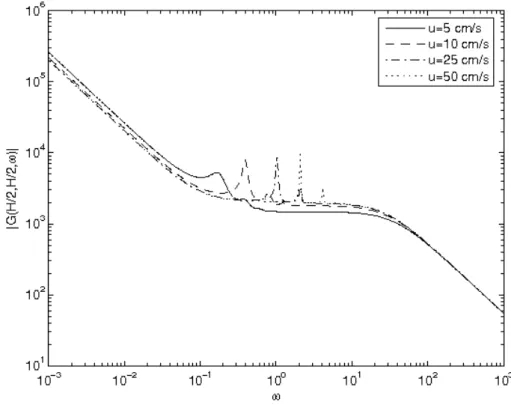
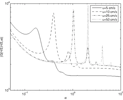
Due to these problems, the space dependence of the solution is not investigated here. A more efficient solution of the problem will be discussed below. Here we only assume that the frequency dependence of the solution is correct, since no similar discontinuity problems are present in the frequency. The frequency dependence of the solution with both the perturbation and the observation point lying in the centre of the reactors, i.e. . The result is shown in Fig. 10 for a few different fuel velocities. Fig. 11 displays the details of the ripples in a different magnification. The calculations refer
/ 2 p
z =z =H
22 (68)
to the same small system in which the quantitative work in Stage 1 and in the former part of this Section was made, such that one can expect point kinetic behaviour up to at least plateau frequencies, depending on system size and other parameters.
Fig. 10. Green’s function for different fuel velocities.
23 (68)
Fig. 11. Details of Green’s function for different fuel velocities.
As can be seen, the frequency dependence of the noise is similar to that of the empirical transfer function, shown in Fig. 10 and Fig. 11, in that it has some ripples at regular frequency intervals. The character of the ripples is, on the other hand, quite different for the empirical transfer function and for the present case. While the peaks were very small and wide in the previous case, here they are quite distinct and narrow. Another difference is that their frequency is related to the total transport time of the fuel through the entire reactor system, as opposed to the empirical model, in which the frequency of the ripples was related to the transit time in the external loop. This indicates that the empirical model represents only a relatively coarse approximation of the true solution. A search for the exact or better form of G ω0( ) will be continued in the next Stage.
1.7 The Green’s function for infinite fuel velocity
For a more efficient solution of the dynamic Green’s function of an MSR, we shall consider the case of infinite fuel velocity, because the equations have a simpler form. The static equation can be solved in a closed compact form. For the Green’s function, a solution method different from the eigenfunction expansion will be used. It is similar to the solution method of the transport equation with a singular source when one seeks a solution with the elimination of the uncollided flux. For the case of infinite fuel velocity, this method also yields a compact closed analytic form solution. In the present Stage this solution will be derived and discussed. The method is possible to extend to the case of finite fuel velocity. This will be investigated in the next Stage.
24 (68)
The equations for infinite fuel velocity can be derived similarly to the static case. The velocity only appears in the integral terms. The only factor for which taking the limit is not trivial is u
(
( ))
( )( ) 1 1 1 , ( ) 1 1 ( ) 1 1 H L i i u i T u e u i u e T u λ ω τ λ ω λ ω λ ω + + − = ⎛ + ⎞ ≈ ⎛ ⎞= + + + − − ⎜ ⎟ ⎜ ⎟ ⎝ ⎠ ⎝ ⎠ 1which leaves us with
(
)
0( ) (1 ) 0( ) 0 ( ) 0 H f f a D z z T φ0 z dz βν φ ν β φ Σ ′ ′ Δ + Σ − − Σ +∫
= (44)for the static case, and
0 0 ( , ) (1 ) ( , ) ( , ) ( , ) ( ) ( ) H f f a a i D z z z dz z v i T z λβν ω δφ ω ν β δφ ω φ ω δ ω λ ω δ φ Σ ⎛ ⎞ ′ ′ Δ + Σ⎜ − − Σ − ⎟ + = Σ + ⎝ ⎠
∫
(45)for the dynamic case. It will simplify things if we change the space variable to
2
H x=⎛⎜z−
⎝ ⎠
⎞
⎟, which means that the system boundaries lie at ±ainstead of 0 and H, where obviously . (Note that earlier x represented the radial coordinate in the two-dimensional case, whereas here it is only a shift of the axial space variable z).
/ 2
a =H
Moreover, the solution of Eq. (44) for the static flux will be symmetric around 0 and fulfil what can be seen as a Poisson equation, which indicates a cosine function with an extra constant term:
( )
0( )x Acos xB0 con φ = + st where B0 f(1 ) a D νΣ −β − Σ= .The boundary conditions then yield
(
)
0( )z A cosB0x cosB a0
φ = −
We must, however, also get an equation for criticality. This is done by noting that the fact that φ0( )z fulfils the static equation, poses the constraint
2 0 0 0 1 cos ( ') ' ( ') ' a a f a a B A B a x dx x dx D T T η ν β φ φ − − Σ =
∫
≡∫
where the notation
0 f
D
η =ν βΣ (46)
was introduced. Carrying out the integration, one arrives at the criticality equation
2 0 0
0 0 0 0
0
2 2
cos a cos sin 0
B A B a B B a T a TB η η + − = (47) 25 (68) SSM 2009:38
We can now use the equation for the time dependant part to obtain the dynamic Green’s functionG x x( , , )0 ω . First, we define
2 2 2 2 0 0 0 ( ) 1 f 1 f a f f i i i B B B B vD v ν ω ω ω ω ν ν ν β ρ∞ ⎛ Σ ⎞ ⎛ Λ ⎞ = − = ⎜⎜ − Σ Σ − Σ − Σ ⎟⎟= ⎜ − − ⎟ ⎝ ⎠ ⎝ ⎠ β and 0 ( ) i λη η ω λ ω = +
Now, we can turn the equation for the Green’s function by taking (45) and replacing the RHS with a Dirac delta:
2 0 0 0 ( ) ( , ) ( ) ( , ) H ( , , ) ' ( ) G x B G x G x x dx x x T η ω ω ω ω ω δ Δ + +
∫
= −The solution of this equation can be sought with a method similar to the elimination of the uncollided flux in the transport equation. The solution is constructed as a sum of two terms. The first is equal to the solution of the inhomogeneous equation but without the last term on the l.h.s., containing an integral. The second is given by the solution of the full homogeneous equation, which will hence contain an arbitrary constant. This constant is determined from the condition that the two terms together have to fulfil the full inhomogeneous equation. We require that both terms fulfil the boundary conditions at x= ±a.
The first of these two terms will hence have the form as the Green’s function of traditional systems; the second will look like the solution for the static flux with replaced by
0
B ( )
B ≡B ω
Hence one can write
(
)
0 0 0 sin ( ) ( , , ) cos cos sin ( ) B a x G x x A Bx Ba H x a x G x B x ω = − +⎧ + x − > < ⎨ ⎩The constants G and H depend on ω and , but not on x. They can be determined from the interface conditions
0 x 0 0 sin( ( )( )) sin( ( )( )) G B ω a x+ =H B ω a x− 0 0 cos ( ) cos ( ) 1 GB B a x HB B a x − + − − =
representing the continuity of the Green’s function and the discontinuity of its derivative, respectively. This gives
0 0 sin ( ) sin ( ) ; sin 2 sin 2 B a x B a x H G B Ba B Ba + − = − = −
The constant A can be obtained from the integral condition. The integral equation is now
26 (68)
2 0 0 ( ) ( , ) cos ( ', , ) ' a a B A x Ba G x x dx T η ω ω ω − =
∫
Carrying out the integrations, we are left with
0 0
0 2
2 2
cos cos cos cos
( ) ( )
( , )
2 ( ) 2 ( ) ( ) cos
cos cos cos sin
Bx Ba Bx B A x aC C T B Ba B Ba Ba Ba T T TB a B K Ba η ω η ω ω ω ω ω − − = ≡ ⎛ + − ⎞ ⎜ ⎟ ⎝ ⎠ If we let ( ) cosx Bx cosBa ϕ = −
when we can write
0 0 0 0 2 0 0 sin ( )sin ( ) ( ) ( ) ( ) 1 ( , , ) sin ( )sin ( ) ( ) cos sin 2 B a x B a x x x C G x x B a x B a x x x T K x B Ba Ba x B ϕ ϕ ω ω ω − + ⎧ = − ⎨ + − > < ⎩ (48)
When ω™ 0 , K( )ω ™ 0, since it will be approaching the left hand side of the criticality equation (47). Since the other term in (48) remains finite,
0 0 0 2 0 0 ( ) ( ) ( , , ) ( ) cos x x G x x TK B B a η ϕ ϕ ω ω ∼
when ω™ 0. Since the Green’s function is now factorised what regards frequency and space dependence, and the space dependence is further factorised into a product of the static flux at x and , respectively, it is shown that an MSR also shows point kinetic behaviour at low frequencies. The analysis can be made similarly with considering systems of decreasing size instead of frequency, with a similar conclusion.
0
x
1.8 Quantitative analysis
The Green’s function for infinite velocities was calculated in a large system, corresponding to a power reactor, for an MRS with infinite fuel velocity, and for a traditional reactor of the same size, which is the same as the MSR with . The calculations were made for various frequencies, and the two cases were compared.
0
u =
Such results can be seen in Fig. 12. At extremely low and high frequencies, the spatial form of the two Green's functions is the same, so they have the same asymptotic properties. At low frequencies, the noise has the same form as the static flux, indicating point kinetic behaviour. However, the amplitude of the Green's function of the MSR is much larger than that in the traditional system. This can be related to the fact that the effective delayed neutron fraction is smaller in the MSR than in a corresponding traditional reactor with the same nuclear constant , due to the fact that a large portion of precursors decays outside the core in the MSR (for sufficiently high transport velocities, this loss is proportional to ). It is easy to show for a traditional system that at plateau frequencies and below, the amplitude of the transfer system is proportional to 1 / . For the MSR, a rough estimate is that the amplitude is
β / L H β 27 (68) SSM 2009:38
proportional with 1 / where takes account for the losses of the decays outside the core.
eff
β β < βeff
One can also observe on Fig. 12 (a) - (d) how the point kinetic behaviour, expressed by the similarity of the space dependence of the Green’s function with that of the static flux, gradually disappears and the system response becomes localized around the perturbation point. It is also seen that the MSR retains a point-kinetic behaviour for larger frequencies than a traditional reactor. This can be attributed to the fact that the MSR is a more tightly coupled system than a traditional reactor, due to the movement of the fuel, which, by transporting delayed neutron precursors from the place of their generation to their decay, establishes a neutronic coupling between different regions.
expressed by the similarity of the space dependence of the Green’s function with that of the static flux, gradually disappears and the system response becomes localized around the perturbation point. It is also seen that the MSR retains a point-kinetic behaviour for larger frequencies than a traditional reactor. This can be attributed to the fact that the MSR is a more tightly coupled system than a traditional reactor, due to the movement of the fuel, which, by transporting delayed neutron precursors from the place of their generation to their decay, establishes a neutronic coupling between different regions.
These results show that, despite many quantitative similarities between the MSR and traditional reactor regarding the static problem and the point kinetic approximation, the space/dependent neutron noise shows significant differences. The fact that the noise amplitude is larger can be transferred to other systems using fuel other than U/235, because in such reactors the fraction of delayed neutrons will be smaller than in the thermal reactors, even with a solid fuel. For an MSR with e.g. thorium fuel, the β will These results show that, despite many quantitative similarities between the MSR and traditional reactor regarding the static problem and the point kinetic approximation, the space/dependent neutron noise shows significant differences. The fact that the noise amplitude is larger can be transferred to other systems using fuel other than U/235, because in such reactors the fraction of delayed neutrons will be smaller than in the thermal reactors, even with a solid fuel. For an MSR with e.g. thorium fuel, the βeffeff will
Fig. 12. Comparison between Green's functions for infinite and zero fuel velocity for various frequencies in a large system (H=300 cm). (a) ω= 0.001; (b) ω= 1; (c)
= 100; (d) ω= 1000 rad/s.
ω
28 (68)
be even smaller, and correspondingly the noise amplitude will be even larger at low and moderate frequencies.
1.9 Conclusions
It was shown that the empirical form for the zero power transfer function of an MRS shows some small irregularities, which are related to the transport time of the fuel in the external loop from the core exit to core inlet. It was also shown, with the use of the traditional zero power transfer function, that in case of different fuel velocities in the core (the existence of a radial velocity profile), the sink structure of the induced noise becomes shallower.
The solution of the space-dependent noise problem was started with the calculation of the Green’s function of the problem. It turned out that the same technique of eigenfunction expansion that was used in the static eigenvalue problem, does not work, because of the singularity of the solution at the perturbation point (discontinuous derivative). The solution showed non-physical spatial oscillations, hence only the frequency dependence could be investigated. This showed that the solution obtained from the space-dependent equations, which is free from the phenomenological simplifications that are used in the empirical transfer function, had much larger and narrower peaks at the inverse of the total recirculation time of the fuel. Hence the validity of the empirical transfer function, used in the literature, is limited.
The space-dependent problem was solved for the case of infinite fuel velocity, with a new technique with separates out a singular and a non-singular term in the solution, similarly to the method of eliminating the uncollided flux in transport problems. A closed analytical solution was obtained for the Green’s function. The technique can also be applied with finite fuel velocity, eliminating the singular term from the eigenfunction expansion, which will then converge much faster. A quantitative study of the solution showed, in a comparison with a traditional system of similar parameters, that the noise amplitude is much higher in an MSR for low and intermediate frequencies, and that the point kinetic behaviour exists for higher frequencies or system sizes than in a traditional reactor.
29 (68)
2 An overview of and introduction to fuzzy logic, and
an application to two-phase flow identification
2.1 General description of the fuzzy logic method
Crisp Logic
In mathematics and crisp logic, it is common for a variable X that takes on values from a given set to be accompanied by a given property. Each value of X is then assigned a clear-cut (yes or no) property value expressing that the value of X either has the property or not. An example is shown for X, the set [0,250]cm of men’s heights and the “tallness” property. Assuming that a man i is tall if xi∈[176,250]cm - and not “tall”
otherwise, that is if xi∈[0,176)cm -, a sharp-edged (crisp) membership function of
“tallness” is produced over the entire range [0,250]cm of X (Fig. 13). This function is well-defined and works nicely for binary operations and mathematics.
However, a number of problems arise in the distinction of membership based on the numerical gradation of X:
• a man of height 176cm is as “tall” as a man of a man of height 210cm;
• a man of height 176cm is “tall”, while a man of height 175.9999cm (i.e. only 10-4cm shorter than the “tall” man) is “not tall”;
• a man of height 145cm is as “not tall” as a man of height 175.9999cm.
In becomes, thus, clear that the binary representation of everyday properties does not always permit their efficient expression.
Fig. 13. Crisp membership function expressing “tallness” in men.
0 50 100 150 200 250 0 0.2 0.4 0.6 0.8 1
crisp membership function
X (height, cm) "t al ln es s " p rope rt y tall 30 (68) SSM 2009:38