Active robust control of wind turbines

ACTIVE ROBUST CONTROL OF WIND TURBINES

by

Copyright by Vahid Rezaei 2014

All Rights Reserved

A thesis submitted to the Faculty and the Board of Trustees of the Colorado School of Mines in partial fulfillment of the requirements for the degree of Master of Science (Electrical Engineering). Golden, Colorado Date: _____________________ Signed: _____________________ Vahid Rezaei Signed: _____________________ Dr. Salman Mohagheghi Thesis Advisor Golden, Colorado Date: _____________________ Signed: _____________________ Dr. Randy L. Haupt Professor and Department Head Department of Electrical Engineering and Computer Science

ABSTRACT

The research work conducted in this thesis focuses on robustness of wind energy conversion system with respect to faults in pitch actuator in order to prevent unnecessary emergency shutdown, and keep the turbine operational without significant inefficiency in its overall performance. The objective is to investigate the feasibility of using a fault estimator and a light detection and ranging (LIDAR) system as additional sensors to design a suitable control system for wind turbines. Robust control technique is used to address these issues.

Three controllers are proposed in this work that try to address sources of inaccuracy in wind turbine operation:

An active fault tolerant controller is first designed using a fault estimator. It is shown that a set of locally robust controllers with respect to the fault, together with a suitable smooth mixing approach, manages to overcome the problem of faults in the pitch actuator.

To address the wind-dependent behavior of turbines, a second controller is designed using the LIDAR sensor. In this configuration, LIDAR provides the look ahead wind information and generates a smooth scheduling signal to provide active robustness with respect to the changes in wind speed.

Lastly, utilizing both the fault estimator and LIDAR, a 2-dimentional wind-dependent active fault tolerant controller is developed to control the wind turbine in region 3 of operation.

The feasibility of the proposed ideas is verified in simulation. For this purpose, the US National Renewable Energy Laboratory’s FAST code is used to model the 3-balded controls advanced research turbine. A discussion on practical considerations and ideas for future work are also presented.

TABLE OF CONTENTS

LIST OF FIGURES ……….………….………. viii

LIST OF TABLES ……….……….. xii

LIST OF ABBREVIATIONS………...……….. xiii

ACKNOWLEDGMENTS ……….………..xiv

CHAPTER 1 ... 1

1.1. Statistical Overview ... 1

1.2. Wind Turbine Overview... 2

1.3. Wind Turbine Control ... 5

1.3.1. Nonlinear Feedback Control ... 6

1.3.2. PID and Optimal Feedback Control ... 8

1.3.3. Robust Feedback Control ... 9

1.3.4. Adaptive Feedback Control ... 10

1.3.5. Feedforward Control ... 11

1.3.6. Fault Tolerant Control ... 13

1.4. Contribution of the Current Work ... 15

1.5. Structure of the Thesis ... 16

CHAPTER 2 ... 17

2.1. A Brief Overview of the Proposed Control Strategy ... 18

2.2. Outline of the Research Work ... 19

CHAPTER 3 ... 21

3.1. Modeling Uncertainty ... 21

3.1.1. Dynamics Uncertainty ... 21

3.1.2. Parametric Uncertainty ... 22

3.3. Passive Robust Controller; An Overview ... 26

3.3.1. Design Issues ... 27

3.3.2. µ Robust Control Design ... 27

3.4. Global Control Signal via Mixing ... 31

3.5. Active Control Design Procedure ... 32

CHAPTER 4 ... 34

4.1. Modeling by FAST Code ... 34

4.2. Unmodeled Dynamics ... 36

4.3. Fault in the Pitch Actuator ... 36

4.4. Wind-Dependent Behavior of Wind Turbines ... 38

4.5. Wind-Dependent Model of Wind Turbines ... 39

4.6. Wind-Dependent Model of Wind Turbines with Fault in the Pitch Actuator ... 41

CHAPTER 5 ... 42

5.1. Pitch Actuator FTC; Design Procedure ... 42

5.2. Design of Local Robust Fault Tolerant Pitch Controller ... 44

5.3. Simulation Verification ... 49

CHAPTER 6 ... 53

6.1. Wind-Dependent Active Robust Controller ... 53

6.1.1. Wind-Dependent Controller; Design Procedure ... 54

6.1.2. Design of Local Robust Wind-Dependent Pitch Controller ... 55

6.1.3. Robustness with respect to LIDAR Measurement Inaccuracy ... 57

6.1.4. Simulation Verification ... 59

6.2. Wind-Dependent Active Robust Fault Tolerant Pitch Controller ... 60

6.2.1. Wind-dependent controller design procedure... 60

6.2.3. 2-Dimentional Mixing of the Local Controllers ... 63

6.2.4. Simulation Verification ... 63

CHAPTER 7 ... 65

7.1. Design Summary ... 65

7.2. Practical Considerations for Field Test on CART3 ... 65

7.3. Future Work ... 67

LIST OF FIGURES

Fig. ‎1.1:Total installed wind energy capacity (in MW) for the period 2010-2013. Reproduced

from ‎[1]. ... 1

Fig. ‎1.2: Distribution of wind power capacity in world. Reproduced from ‎[1]. ... 2

Fig. ‎1.3: CART2 and CART3. Picture courtesy of NREL. ... 3

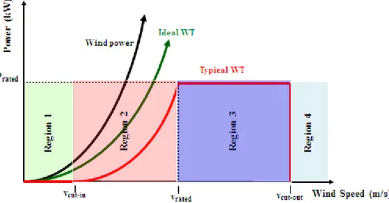
Fig. ‎1.4: Regions of operations in WTs. The wind power is proportional to the cube of wind speed (black curve); however, theoretically, a WT can absorb up to only 59% of the wind power (green curve). The red curve shows the power curve of a typical wind turbine with Cp<0.5. ... 5

Fig. ‎1.5: CART’s Cp surface as a function of pitch angle and tip speed ratio. ... 6

Fig. ‎1.6: Interconnection of subsystems in a WT and the effects of the environment. Modified from ‎[10], with permission. ... 7

Fig. ‎1.7: Nacelle mounted LIDAR configuration, adopted from ‎[55] with permission. ... 12

Fig. ‎1.8: Direct LIDAR-based control of WTs. ... 12

Fig. ‎1.9: Passive vs. active FTC. Both passive and active control ideas can be used to design a controller. ... 14

Fig. ‎1.10: Passive vs. active control, non-intersecting case. Only active control technique has a solution for this problem. ... 14

Fig. ‎2.1: Uncertain wind-dependent model of the augmented actuator-WT with fault in the actuator. The complex-valued unmodeled dynamics uncertainty , real-valued wind-dependent uncertainty and real-valued fault uncertainty are separately addressed in this approach.19 Fig. ‎2.2: General scheme for the mixed design ... 19

Fig. ‎3.1: Multiplicative uncertainty representation. ... 22

Fig. ‎3.2: General scheme of active robust control. ... 25

Fig. ‎3.3: Real [red] vs. complex-valued [blue] uncertain models. ... 26

Fig. ‎3.4: General configuration for robust control design. ... 28

Fig. ‎3.5: General configuration for robust stability analysis. ... 28

Fig. ‎3.6: General configuration for robust performance problem. ... 29

Fig. ‎3.7: General scheme for mixed design ... 29 Fig. ‎3.8: The big picture to show how active robust conrol design in (b) can provide theretical guarantees on a wide range of changes in parameters with fewer number of local controllers

comparing to the non-robust cotrol design in (a). In (a), different controllers are designed at intersections of vertical and horizontal blue lines while in (b), each controller guarantees robustness for one square. In both non-robust (a) and robust (b) control ideas, the activeness is

achieved through the switcihng betwee the local controllers. ... 33

Fig. ‎4.1: Augmented pitch actuator-WT model. ... 36

Fig. ‎4.2: Uncertain augmented pitch actuator-WT model. ... 36

Fig. ‎4.3: Step responses of different actuator models given the parameters in Table ‎4.2 ... 37

Fig. ‎4.4: Uncertain augmented pitch actuator-WT model with complex-valued unmodeled dynamics uncertainty and real-valued fault uncertainty . ... 38

Fig. ‎4.5: Change in pole locations of CART3 by wind speed (Red: 14 m/s and Blue: 24 m/s). .. 39

Fig. ‎4.6: Change in BW by wind speed. ... 39

Fig. ‎4.7: Uncertain wind-dependent modeling of the augmented actuator-WT with complex-valued unmodeled dynamics uncertainty and real-complex-valued wind-dependent uncertainty . .. 40

Fig. ‎4.8: Uncertain wind-dependent model of the augmented actuator-WT with fault in actuator. The complex-valued unmodeled dynamics uncertainty , real-valued wind-dependent uncertainty and real-valued fault uncertainty are separately addressed in this approach.41 Fig. ‎5.1: Closed-loop form of the proposed robust control structure... 44

Fig. ‎5.2: Power spectrum density of a typical wind speed profile. Most of the wind speed energy is concentrated at low frequencies. ... 45

Fig. ‎5.3: Open-loop structure should be used to find the generalized plant P(s). The uncertainty blocks are removed and the controller needs to be designed (all these blocks are shown with dashed red lines). ... 46

Fig. ‎5.4: Requred configuration to design local FTCs. The generalized plant P(s) includes the weighting functions, WT and the actuator models. ... 46

Fig. ‎5.5: Bode magnitude plot comparison of the full order and reduced order models for the 16thlocal controller. For reference tracking purposes, the controller shows the required integral action property at low frequencies. ... 48

Fig. ‎5.6: Closed-loop wind energy conversion system with FTC... 49

Fig. ‎5.7: Simulation results of FTC with mixing. ... 50

Fig. ‎5.9: Tower fore-aft acceleration (top) and tower side-to-side acceleration (bottom) for the given fault scenario. ... 52 Fig. ‎5.10: Blade 1 moments for the given fault scenario. ... 52 Fig. ‎6.1: Indirect LIDAR-based control of WTs... 54 Fig. ‎6.2: Open-loop structure for wind-dependent design. The controller should be designed with the uncertainty blocks removed (all these blocks are indicated with dashed red lines). This configuration is used to find the generalized plant P(s). ... 56 Fig. ‎6.3: Required configuration to find the local wind-depedndent controllers via DK-algorithm. Generalized plant P(s) includes the weighting functions, WT and the actuator models. ... 56 Fig. ‎6.4: Proposed LIDAR-based wind-dependent controller (WDC) for WTs. ... 57 Fig. ‎6.5: Using the overlap to provide robustness with respect to the LIDAR inaccuracy. The actual (solid red line) and measured (dashed red curve) wind speed parameters are drawn for the worst case scenario. ... 58 Fig. ‎6.6: Generator speed regulation with BLC (blue) and LIDAR-based (red) controllers. ... 59 Fig. ‎6.7: Required pitch actuation signals for the given wind file by BLC (blue) and LIDAR-based (red) controllers... 60 Fig. ‎6.8: Localization of the wind-dependent active robust FTC. The length of all intervals are predetermined and fixed. ... 61 Fig. ‎6.9: Open-loop structure for wind-dependent design. The controller needs to be designed with uncertainty blocks removed (all these blocks are indicated by dashed red lines). The generalized plant should be generated from this figure. ... 62 Fig. ‎6.10: Generalized plant for local wind-dependent active robust FTC synthesis. ... 62 Fig. ‎6.11: Comparison of wind-dependent active FTC (dashed red) and active FTC (solid blue). Fault parameter, generator speed (rpm) and rotor speed (rpm) are shown from top to bottom.... 63 Fig. ‎6.12: Comparison of wind-dependent active FTC (dashed red) and active FTC (solid blue). Pitch angle, pitch rate (deg./s) and pitch accelleration (deg./ ) are presented from top to bottom. ... 64 Fig. ‎7.1: A bad transition between regions 2 and 3. The top plat is a hub height wind speed that goes back and forth between the two regions. The other two plots represent the corresponding rotor and generator speed signals with the active robust FTC in the loop. ... 66

Fig. ‎7.2: An anti-windup transition algorithm is developed for active FTC design for a wind profile with mean of 14.5 m/s and turbulent intensity of 17%with a fault scenario as Fig. ‎7.1. The anti-windup strategy prevents instability and keeps the pitch actuation within acceptable limits. It should be noted that when the wind speed passes to region 2, the generator and rotor speeds drop since the wind does not have enough power to turn the turbine at its rated speed. ... 68 Fig. ‎7.3: Robust adaptive fault parameter estimation for a second order parametric model of the pitch actuator with noisy measurement... 69

LIST OF TABLES

Table ‎4.1: DOF provided by FAST code to model the mechanical and electrical subsystems of a 3-bladed on-shore wind turbine. Aerodynamic Torque calculation has its own DOF (not shown

in this Table). ... 34

Table ‎4.2: Fault parameters for the second order actuator model of the turbine. ... 37

Table ‎5.1: Maximum achievable Cf. ... 47

Table ‎5.2: Local robust FTCs ... 48

Table ‎6.1: Local robust controllers for wind-dependent design. ... 57

Table ‎6.2: Summary of numerical verifications. The improvements are in comparison with the BLC. ... 60

LIST OF ABBREVIATIONS

BLC ………... Baseline controller CART2 …….……….… 2-bladed controls advanced research turbine CART3 …….………....…. 3-bladed controls advanced research turbine DEL ……….….………. Damage equivalent load DOF ……….. Degree of Freedom DTC ……… Disturbance tracking control FAST ……….……….… Nonlinear aero-elastic turbine simulation code FDI ……….. Fault detection and isolation FTC ……… Fault tolerant control HAWT ………...………. Horizontal axis wind turbine LIDAR ………...……….. Light detection and ranging LPV ……….… Linear parameter varying LTI ……….. linear time invariant MMC ………..……… Multiple-model control MPPT ……… Maximum power point tracking NREL ……….….. National renewable energy laboratory NWTC ………..………... National wind technology center PID ……….……… Proportional integral derivative QFT ……… Quantitative feedback theory RMS ………..……….. Root mean square VAWT ………..……….. Vertical axis wind turbine VSWT ………..……….……….. Variable speed wind turbine WECS ………..………. Wind energy conversion system WT ………..………… Wind turbine

ACKNOWLEDGMENTS

I would like to thank my advisor, Dr. Salman Mohagheghi, for his help, guidance and faith. Also, my deep gratitude goes to Prof. Kevin Moore for his help during the time I was a graduate student at Colorado School of Mines. Additionally, many thanks to Prof. Tyrone Vincent for serving on my thesis committee. Also, I would like to thank Prof. Kathryn Johnson for her comments regarding my simulation work on active robust controllers for wind turbines. Finally, it should be mentioned that this work was partially supported by the US Department of Energy under award number DE-SC0004267, subcontract number C1910-050112, for which I am grateful.

CHAPTER 1

The general trend in wind technology is discussed in this chapter starting with an overview of global wind energy capacity. Different types of wind turbines (WTs) and their operation regions are then introduced with the goal of presenting the main control objectives and potential control inputs for each region. In addition, the challenges in control of WTs are highlighted through a survey of the state-of-the-art in WT control. The chapter will conclude with a description of the structure of the thesis.

1.1.Statistical Overview

As a clean alternative to fossil fuels, renewable energy has attracted considerable interest among the power grid operators and policymakers within the past 10 years, to the extent that the installed capacity of renewable power exceeded 1470 GW at the end of 2012[1]. As a fast growing renewable energy resource, wind energy continues to contribute to the power grids around the world, with a total capacity of 296,255 MW by the end of June 2013, i.e., amounting to 3.5% of the global electricity demand [1]. Figure 1.1depicts the total installed capacity of wind energy during the period from 2010 to 2013 [1].

Fig. 1.1:Total installed wind energy capacity (in MW) for the period 2010-2013. Reproduced from [1].

Figure 1.2 shows the top markets of wind technology in the world in 2013 [1]. The market for wind energy in the United States was assisted by the increasing trend in manufacturing

End 2010 Mid 2011 End 2011 Mid 2012 End 2012 Mid 2013 Expected by end 2013 199739 218144 237717 254041 282275 296255 296255

turbine components, in addition to improvements in WT design which could lead to increased turbine efficiencies. Around 45% of all new electricity generation in the US is based on wind energy [2]. To be able to respond to larger demands, the size of the turbine would have to be increased; for example a typical 5 MW WT has a tower of approximately 114 m high, with a rotor diameter of 124 m [3]. However, increasing the size of WTs would result in an increase in its overall cost. This in turn calls for advanced control strategies that enable the turbine to achieve more electrical energy from the available wind, while at the same time reducing the maintenance cost.

Fig. 1.2: Distribution of wind power capacity in world. Reproduced from [1]. 1.2.Wind Turbine Overview

A WT works based on the principles of lift and drag forces as a result of wind blowing towards the turbine blades. These forces turn the turbine, and therefore the rotor of the generator which is coupled to the turbine, thereby producing electrical energy. Based on the configuration and layout of the blades and their rotation plane, WTs are classified as vertical axis wind turbine (VAWT) or horizontal axis wind turbine (HAWT). HAWT is more complex and more expensive than VAWT; however, it is more popular due to its higher efficiency. In terms of the way the generator rotor is connected to the turbine’s rotor, a WT can be classified as direct-drive, where the turbine’s rotor is directly coupled to the electrical generator, or gearbox-based, where the gearbox divides the power shaft into a low speed shaft on turbine side and a high speed shaft on the generator side. In this thesis, a gearbox-based HAWT is used in the analysis mainly due to its popularity in wind industry. Figure 1.3 shows the 2 and 3-bladed controls advanced research

turbines (CART2 and CART3) of the US national renewable energy laboratory (NREL) located at national wind technology center’s (NWTC) wind farm near Boulder, CO.

The main components of a HAWT are:

1. Hub and Blades: The blades convert the wind energy to rotational displacement, and hub connects the blades to the low speed shaft.

2. Low-Speed Shaft: This shaft connects the rotor to the gearbox.

3. Gearbox: Connects the low-speed shaft to the high-speed shaft. It increases the rotational speed of low-speed shaft to make it match the required rotational speed of the generator. 4. High-Speed Shaft: This connects the gearbox to the electrical generator to allow for the

conversion of mechanical energy into electrical energy. 5. Electrical Generator: Produces electrical energy.

6. Brakes: Are used to stop the WT either at normal or emergency situations.

7. Nacelle: This is where the low and high speed shafts, the brakes, the generator, and other relevant components are located.

8. Tower: Since there is more wind power at higher elevations, the tower lifts the rotor and nacelle up to an optimum level above the ground.

In addition to the classifications mentioned earlier, a HAWT can be a fixed-speed WT or a variable-speed WT (VSWT). In the case of the latter, the WT can be further subdivided based on the type of control scheme, namely, stall control, active stall control or pitch control [4]. The fixed-speed WTs are simple in design, are cheap, can be directly connected to the grid, and can be designed in such a way that the maximum aerodynamic efficiency of the turbine is achieved at a fixed speed. However, pitch-controlled VSWTs are selected in this study due to the fact that their power electronics interface makes it possible to study the WT independent of the power grid dynamics and the related frequency issues, and provides a better control authority on a wide range of wind speeds.

To better determine the control objectives, the operational regions of the WT are often divided into different regions as described below (see Fig. 1.4) [5]:

1. Region 1: At this region, wind speed is below the cut-in value and the wind power is not enough to turn the rotor. Here, the pitch angle is set to produce the minimum aerodynamic torque, and the turbine is off-work.

2. Region 2: An increase in wind speed increases the wind power, and the rotor starts to turn. Now, the pitch angle is kept at its optimum value in order to produce the maximum aerodynamic torque. At this region, the control input is limited to the generator torque command in order to achieve maximum power point tracking (MPPT) via control of the generator speed.

3. Region ⁄ : This is a fictitious region where the wind speed is getting close to its rated value and is often modeled to assist with a smooth transition between regions 2 and 3. Here, the generator torque command is calculated such that the rated power of the generator will be achieved at rated wind speed. As a result, mechanical stress will be decreased with a safe switching approach. Normally, both pitch angle and generator speed are considered the control inputs at this region.

4. Region 3: Here, the wind speed is above the rated value, and the control mechanism starts to limit the power absorption. The torque input is constant and the pitch command input is utilized in order to control the rotor speed and consequently maintain the aerodynamic power at its rated value. Power regulation, mechanical load reduction and safe operation are the main objectives at this region.

5. Region 4: At this region, wind speed exceeds the cut-out value and the turbine falls into its normal shut-down process. Usually, loads on WTs which result from the high wind speed, and the safety concerns at shut-down time are the main operation challenges at this region.

Fig. 1.4: Regions of operations in WTs. The wind power is proportional to the cube of wind speed (black curve); however, theoretically, a WT can absorb up to only 59% of the wind power (green curve). The red curve shows the

power curve of a typical wind turbine with Cp<0.5.

From a mathematical point of view, the rotor of a turbine absorbs wind power through equation (1-1) (1-1)[6].

( ) ( ) (1-1)

where is the rotor power, is tip speed ratio which is defined as the ratio of rotor tip speed to the wind speed, is the air density, is the length of the blades, is the wind speed, is the power coefficient of the turbine, and is the rotor speed. Figure 1.5 shows the coefficient for CART which is obtained by WT-Perfcode [7].

1.3.Wind Turbine Control

A survey of literature on advanced control strategies for WTs indicates the following as the main design challenges:

1. Wind disturbances affect the performance of the closed loop system.

3. The main source of the nonlinearity in WTs, i.e. the function, is unknown, and changes during the course of operation of a WT.

4. WT dynamics indicate wind-dependent behavior, which means that the parameters of a WT model are different at different wind speed operating points.

5. Wind speed estimation or light detection and ranging (LIDAR) measurements of wind speed may have inaccuracies.

6. Faults may occur in the components of the wind energy conversion system (WECS). In the rest of this chapter, the strategies adopted in the literature to address some of these challenges are briefly pointed out.

Fig. 1.5: CART’s Cp surface as a function of pitch angle and tip speed ratio.

1.3.1. Nonlinear Feedback Control

As illustrated in Fig. 1.5, the surface is a nonlinear function of the pitch angle and the tip-speed ratio (or rotor tip-speed and wind tip-speed). Consequently, aerodynamic torques and bending moments are nonlinear functions of wind speed, pitch angle and rotor speed [5]. This would naturally indicate that precise reference tracking in WECS can be better achieved through nonlinear control methodologies.

0 10 20 30 2 4 6 8 10 12 14 0 0.1 0.2 0.3 0.4

 [Tip Speed Ratio]  [Blade pitch angle]

Cp [ P o e w e r c o ff ic ie n t]

This issue has been addressed in the literature. For example, a feedback linearization control strategy was introduced in [8] to handle the problem of nonlinearity in WTs and to separate the wind disturbance from the dynamics of the turbine. The authors used the same model for both controller design and simulation, and reported promising results.

WTs are complex systems with many subsystems and coupled modes as depicted in Fig. 1.6 where not all of these modes are considered in the design process of the controller. However, these unmodeled dynamics may adversely affect the stability and performance of the overall closed-loop system. For example, a similar feedback linearization method as in [8] was adopted in [9] to control the CART coded with FAST; however, it led to different results. These mismatches between the results can be due to adoption of a simplified WT model for controller design purposes, which can further underline the effect of unmodeled dynamics as one of the controller design challenges.

Fig. 1.6: Interconnection of subsystems in a WT and the effects of the environment. Modified from [10], with permission. Aerodynamics Loads on WT Soil-WT structure reactions WT Control systems Rotor dynamics Wind Effect of Environment Soil Drive-Train dynamics Power generation dynamics Foundation dynamics Nacelle dynamics Tower dynamics

Another source of inaccuracy in the design of feedback linearization based controllers comes from the assumption of having an analytical function for . Although it is common in the literature to assume a known surface and accordingly design nonlinear or lookup-table-based strategies for control of WTs [11],this function is in general unknown and furthermore, it changes over time for an installed WT [12]. This means that control systems designed based on the assumption of known Cp may not be reliable for the purpose of long-term operation;

although, more efficient controllers may be able to address this issue to some extent. For example, in [13], sliding mode nonlinear control strategy was adopted as an alternative for feedback linearization technique. This controller is inherently robust with respect to either nonlinearity in the behavior of the system or the effect of disturbances. However, chattering in the controlled output may impose some restrictions on pitch actuators and therefore question the feasibility of such controllers for control of WTs at region 3. By increasing the complexity of the original design, the authors of [13] introduced a higher order sliding mode controller combined with a sliding mode observer in order to solve the chattering problem for generator torque control of WTs [14]. In another case, a novel nonlinear control method has been developed in [15] to control both speed and power of the generator in a cascaded configuration. Also, in order to increase the captured energy and decrease the mechanical load, Kalman filtering was used in [16] in combination with a nonlinear dynamics state feedback controller.

Regardless of the results, as also noted in [17]-[18], using a nonlinear controller may lead to instability or limit cycle issues as well as the lack of realizable analytical solutions. Hence, while WT has a nonlinear behavior and it is verified through simulations that nonlinear control methods improve the performance of WECSs, in practice, linear controllers tend to be more popular within the wind industry.

1.3.2. PID and Optimal Feedback Control

It is easy to show that a proportional integral derivative (PID) controller is robust with respect to constant disturbances. Therefore, under the assumption of having piecewise constant wind disturbances, PID has been widely used to control WTs. PID-based control of WT is discussed in detail in [19]. However, since the linearized WT model depends on the wind speed parameter, even in the absence of any unmodeled dynamics, the parameters of a WT model would vary from one wind speed operating point to another. This means that a PID would not be able to provide any guarantees for general stability of the linear WECS. In order to solve this

problem, gain-scheduled PID has been used to control the WT [20]-[22]. The basic idea is to design different PIDs at different wind speed linearization points and find a scheduling function based on interpolation of the controllers in order to adjust the loop gain appropriately. In this technique, pitch angle and wind speed can be considered as the scheduling parameters. Although this controller shows improved performance in comparison to the conventional approach; similar to the PID method, the design would be sensitive to the unmodeled dynamics.

Other control techniques have also been proposed in the literature. For example, authors in [23] apply a novel multivariable controller to control CART with the objective of achieving reasonable power regulation while ignoring modeling uncertainties. In other instances, researchers have used multivariable control theory in order to satisfy multiple objectives simultaneously. Authors in [24] simulated a optimal control for WTs without considering modeling uncertainties. Authors of [21] and [25]-[30] used the theories of disturbance tracking control (DTC), disturbance accommodating control and disturbance utilization control in state-space in order to solve the multi-objective control problem of WTs. Since they estimated the wind speed, these methods were efficient in reducing the effect of wind disturbances; however, wind-dependent behavior of WTs was not considered in their analysis.

The concept of DTC was enhanced in [31] in order to address the periodic behavior of WT dynamics. However, this would still be ineffective with regards to the unmodeled dynamics of the WT. In order to achieve to a better closed-loop performance, a higher-order model of WT is required that inevitably increases the complexity of the design procedure. Moreover, in this case, the need for observability would force the designer to utilize additional sensors which would in turn add to the cost of the controller.

1.3.3. Robust Feedback Control

As pointed out in [6] for CART, unmodeled dynamics may lead to poor performance and instability of the WECS. To address this and in order to be able to control plants with modeling uncertainties, passive robust control methods have been adopted [32]-[33]. Geng and Yang [34] introduced a nominal inverse-model based controller augmented by a robust compensator to mitigate the effects of nonlinearities and the disturbances. Using this approach, they achieved a robust tracking of the power command. Quantitative feedback theory (QFT) is another robust control methodology in frequency domain which uses feedback values in order to either reduce

the effect of modeling uncertainties or satisfy the desired performance of the closed-loop system. This idea was applied to control of WT in [35]. Nevertheless, these solutions do not consider the wind-dependent dynamics of the turbine. To make matters worse, conventional robust controllers lead to very conservative designs for WTs, especially if all aforementioned design challenges are taken into account.

Linear parameter varying (LPV) control is another scheme which has been used in the literature to maximize the energy captured, address the unmodeled dynamics of WTs, and consider its wind-dependent behavior [36]-[40]. This method addresses all aforementioned challenges in linear control of WTs while assuming a measured or estimated wind speed as an independent parameter. In another instance, the author of [35] developed a switching-QFT robust controller to enhance the QFT controller proposed in [18]. Also, authors in [41] designed a multiple-model controller (MMC) for distinct wind speed linearization points to consider the wind-dependent behavior of WTs. However, this approach is not robust with respect to the unmodeled dynamics, and the overall performance is sensitive to the accuracy of wind speed estimation. Additionally, this does not provide any guarantees for transients from one wind speed operating point to another.

1.3.4. Adaptive Feedback Control

Adaptive control could partially solve the problem of wind-dependent behavior of WTs. This method has been evaluated in [42]-[48] and [51]-[53]. Authors of [42] applied a self-tuning regulator as a step towards adaptive control of WT. A generalized model predictive control was used in [43] as another adaptive approach for pitch control of WTs. A multi-input multi-output self-tuning regulator was simulated in [44] to regulate the output power, and also to decrease the load on WT. Authors of [45]-[47] argued that the uncertainty in the aerodynamic parameters of a WT may lead to non-optimality in tracking of maximum power points of WT. To address this, they used adaptive control ideas to find optimal solutions that could overcome the lack of knowledge about aerodynamic properties of WTs. All these methods showed improvements; however, in general, they do not provide guarantees for stability and performance with respect to unmodeled dynamics. In [48], direct adaptive control strategy of [49] was modified to regulate the generator speed of CART at its rated value while considering wind speed disturbance. In addition to the modeling uncertainty, the main difficulty of this method lies in its assumption on

having a strictly positive real system which may restrict its applicability [50]. However, this problem is solvable for single-input single-output model of WT. In [51], the method of [48] was improved to separate the non-strictly positive modes from other modes in order to overcome the previous problem and consider the structural modes of WTs. Also, adaptive DTC was developed in [52] to relax the assumption of having a WT with known parameter values, and was applied for torque control of CART. In [53], an adaptive partial state feedback DTC augmented with wind speed estimator was developed and applied to NREL’s 5MW WT. Due to the complexity in the design of adaptive controllers for turbulent wind profiles, the simulations were limited to a step-like wind speed profile. Nevertheless, these methods are still not considered robust with respect to modeling uncertainties.

To simultaneously address the unmodeled dynamics uncertainty, wind-dependent behavior of WTs, and wind disturbance input in the linear control of WTs, the authors of [54] modified the conventional feedback robust model reference adaptive control idea of [50] and developed a robust adaptive feedback-feedforward pitch controller for CART. Here, the feedforward term was based on adaptive estimation of the changes in wind speed, and the method was verified for both step-like and turbulent wind profiles.

1.3.5. Feedforward Control

As an alternative approach for estimation of wind speed, Fig. 1.7 shows how the LIDAR sensor provides information about the wind speed at a distance in front of the turbine [55]-[57]. In many references, researchers have used LIDAR information for control of WTs, where a trade-off is made between the reference tracking (or regulation) and mechanical load minimization in order to achieve to their control objectives[58]-[60]. The ideas are very similar to each other and follow the feedforward control theories. These strategies are referred to here as direct LIDAR-based control of WTs, as represented by Fig. 1.8. This configuration allows for redesigning the original feedback part with the goal of reducing the required actuation signals [61]. In another work, [62] used a LIDAR-based model predictive control loop in addition to the preview feedback controller in order to improve some of the performance indices in control of WTs. However, LIDAR measurement inaccuracies together with the effect of unmodeled dynamics and disturbances in the measurement path can magnify the effect of modeling uncertainties in the feedback loop and may lead to instability of the WECS.

Fig. 1.7: Nacelle mounted LIDAR configuration, adopted from [55] with permission.

Fig. 1.8: Direct LIDAR-based control of WTs.

The authors of [63] used optimal filtering approach to reduce the effect of measurement errors on direct LIDAR-based control schemes. They showed that LIDAR measurement errors in the conventional feedforward strategy could degrade the performance of the closed-loop system. However, they did not consider the unmodeled dynamics or the wind-dependent behavior of the WT model. WT LIDAR Feedback control Feedforward control 𝑢 Wind Measurements

1.3.6. Fault Tolerant Control

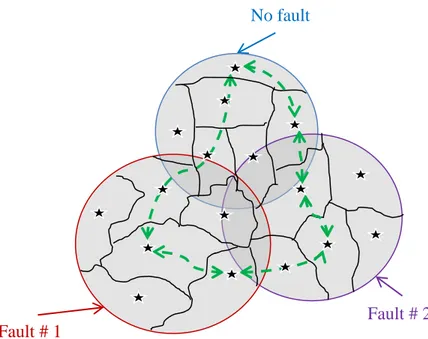
Regardless of the efficiency of the control ideas discussed earlier, WECSs need different sets of sensors and actuators in order to implement the control schemes. These components are subject to different abnormalities and faults. It is therefore important to investigate the effects of actuator and sensor malfunctions on the general behavior of the closed-loop system (e.g., on power tracking error), and design a controller that enables the WECS to operate successfully in the presence of these unwanted situations. Fault tolerant control (FTC) is a well-researched topic in the control systems literature and is suitable to compensate for these abnormalities [64]-[66]. FTC is typically divided into two groups: passive and active, as is illustrated in Fig. 1.9 [66]. Passive control uses different robust control methodologies to address the problem of faults with only a single controller. On the other hand, active control usually includes a fault detection and isolation (FDI) unit in addition to estimating one or more fault parameters and actively tuning the control signal based on fault conditions. Here, FDI is used to identify the plant condition and send the required commands to the plant accordingly.

To further describe Fig. 1.9, three different cases have been assumed: normal (no fault), fault #1, and fault #2, which are distinguished from one another by using different colors. Each circle shows the possible set of controllers for the corresponding case, and the stars represent the best controller for each scenario. Active FTC would then make it possible to switch among the stars while passive FTC would be restricted to the intersections of solutions for all cases. Hence, while the closed-loop performance by a passive FTC is limited (even for the no fault case), the system works with its best possible performance for different cases under an active FTC. Simplicity in design and implementation of the passive controllers is its main advantage, whereas active FTC is characterized through superior performance. However, the main drawback of passive FTC is the fact that, similar to any other robust control technique, the general solution is only available when the local solutions intersect. Figure 1.10 demonstrates this drawback of passive FTC where it has been shown that active FTC is able to handle the non-intersecting case.

Despite the fact that FTC is widely used in different applications, it is relatively unexplored within the WT field of study. Much of the work in this field focuses on FDI techniques [67]-[71] and is based on the first WT fault tolerant benchmark model presented in [72]. Few instances have been reported on WT FTC [39],[40] and [54]. However, as discussed in [73], it is desired

for WTs to keep working under faulty conditions, which further justifies the need to investigate the FTC techniques for WTs. This is the main topic of the research work presented here.

Fig. 1.9: Passive vs. active FTC. Both passive and active control ideas can be used to design a controller.

Fig. 1.10: Passive vs. active control, non-intersecting case. Only active control technique has a solution for this problem. Possible solutions # 0 Possible solutions # 1 Possible solutions # 2 No Fault Fault # 2 Fault # 1 Best possible solution # 0 Best possible solution # 1 Best possible solution # 2 Passive Control Active Control Possible solutions # 0 Possible solutions # 1 Possible solutions # 2 No fault Fault # 2 Fault # 1 Best possible solution # 0 Best possible solution # 1 Best possible solution # 2 Passive Control ? Active Control

1.4.Contribution of the Current Work

From an application point of view, based on the author’s best knowledge, the proposed design is the first active robust controller to address the problems of fault in the actuator, wind-dependent dynamics behavior, and wind speed disturbance. In particular:

1. The main objective of this research is to design fault tolerant pitch controller for control of WTs at region 3 of operation. Since the information about different faulty cases is available, LPV modeling is used to describe pitch actuator based on a fault parameter. Then, a set of local robust controllers are designed that are passively robust against local changes in the fault parameter. To globalize guarantees for robustness against faults, a fault estimator is used to measure the fault parameter. Then, this measured parameter is used to actively determine the correct local controller within the loop. It should be mentioned that the final controller is passively robust against unmodeled dynamics. Additionally, reducing the effect of wind speed disturbances on the measured generator speed is the other control objective that is guaranteed through utilizing robust control technique. Furthermore, assuming a fixed design structure, an innovative idea is proposed to systematically determine the number of local passive controllers through an iterative approach.

2. Proposed active design idea is used to address the problem of wind-dependent dynamics in WTs. In this case, a wind speed dependent LPV model is formulated to design different local controllers. Then, LIDAR wind speed measurement is used as the scheduling signal to adaptively change properties of closed-loop WECS depending on wind speed operating point.

3. The previous two designs are combined to adaptively adjust properties of the closed-loop WECS based on fault and wind speed parameters. Here, similar to the second design, it is important to capture parameter-dependent properties of WT’s dynamics. Thus, the systematic local linear model design procedure of FTC controller is no longer applicable. Remark: It should be noted that the systematic procedure proposed in FTC design could be used for wind-dependent designs in order to determine the number of local controllers based on the required disturbance rejection property of the closed-loop system. However, it is preferred to predetermine the number of local controllers and instead, capture the wind-dependent behavior of the WT’s dynamics through the change of the weighting functions.

1.5. Structure of the Thesis

The rest of this thesis is organized as follows: Problem statement is presented in Chapter 2. Chapter 3 provides a literature survey on available strategies suitable to meet the control objectives of this research. The basics of the theory behind the proposed control idea are also introduced in this chapter. Chapter 4 formulates the WT problem and sets the design requirements. To investigate the feasibility of the proposed method, the simulation results are presented in Chapters 5 and 6. Finally, Chapter 7 discusses the practical consideration issues, implementation requirements, as well as concluding remarks and suggested future work to continue this research.

CHAPTER 2

Based on the discussion of Section 1.3, the following list is now introduced as the main technical challenges in controlling WTs:

1. Unknown time-varying nonlinearity in WTs,

2. The effect of wind disturbance on the performance of the closed-loop system,

3. The effects of unmodeled dynamics on the stability and performance of the closed-loop system,

4. Wind-dependent WT dynamics,

5. Faults in the components of the WECS, 6. Inaccuracy of the LIDAR measurements.

The objective of this research is not to simultaneously address all the above design issues; however, as discussed below, it is intended to fully or partially resolve some of these concerns.

The first design challenge points out that the nonlinear model-based control strategies that use the function are not necessarily reliable. Robust nonlinear control strategies could be investigated instead in order to find a solution for this problem. These designs are not considered here; although, they have been addressed in the literature for general nonlinear systems.

With or without LIDAR, the second design issue has generally been addressed in the WT literature through adopting feedforward strategies. As an alternative to direct LIDAR-based control strategies, the solution pupt forth in this research can be seen as another technique for wind speed disturbance rejection. In the proposed solution, this control objective is achieved by defining the desired control performance without wind speed measurement.

The third design issue is completely well-known in the control theory literature, and is usually addressed through utilization of robust control techniques. Robust control is the foundation of the proposed solution in this research.

The fourth and fifth design issues highlight the uncertainties in the parameters of WT linear models. An appropriate control technique needs to be designed based on a suitable parameter-dependent model for the WT. LPV and gain-scheduling techniques have traditionally been used for problems of this nature, and may be suitable for the purpose of WT control as well. However, robust adaptive control strategies are in general considered to be superior in the presence of

uncertainties, yet, there is only one reference that partially considers the above issues by using robust adaptive schemes in the time domain [54].With the goal of achieving a better performance, the scheme proposed here is developed in the frequency domain, as further discussed in Chapter 3.

Due to its importance, the fifth design challenge has also attracted a lot of attention in the literature, and is well-researched. The proposed methodology here, although not the only solution, is able to address these fault conditions as well.

The sixth challenge is investigated in [63] for direct LIDAR-based techniques. This aspect is also addressed in the proposed control strategy without introducing any additional complexities in the controller design.

2.1. A Brief Overview of the Proposed Control Strategy

Active robust control technique adopted in this research is a special case of robust adaptive control schemes, and potentially is able to address design challenges 2 through 6 discussed in the previous section. For this reason, this technique has been proposed and analyzed here as a possible solution for the WT control application. In this approach, advantages of frequency domain robust design can be further enhanced with the time-domain properties of the active control concept. In the frequency-domain, different, and sometimes contradictory, design objectives can be satisfied through an appropriate design tradeoff, while in the time-domain, the conservativeness of the design can be reduced by considering parametric uncertainties separately. More specifically, in the frequency-domain, the mixed -robust control formulation is used as a tool that provides guarantees for both robust stability and robust performance by the use of maximum possible knowledge of the WT model. This basically results in an in-depth model-based control design, and has a less conservative design compared to conventional robust control approaches.

The big picture for this design is as follows:

1. A suitable WT model for robust control design purposes is developed here as illustrated in Fig. 2.1, where the required notation for this figure is discussed in detail in Chapter 4. 2. Robust mixed synthesis method is determined to be suitable to solve the design

problems of this thesis. In order to apply this technique, the model in Fig. 2.1 is augmented with some weighting functions (see Chapters 5 and 6) and transformed into the generalized plant P(s) as illustrated in Fig. 2.2. Then, the robust stability and robust

performance are locally guaranteed by robust control theory. Further information about this method is described in detail in Chapter 3.

3. To globalize the robustness guarantees, a mixing (bumpless switching) scheme is applied in order to generate the global control signal based on a set of local control signals. The general idea of this approach is introduced and discussed in Chapter 3.

4. This technique has been applied here for designing FTCs for WT application in Chapters 5 and 6. In all cases, generator speed is considered to be the measured signal, and the blades’ collective pitch angle is the control input to the WT. In addition, fault and wind parameters are measured by the fault estimator and the LIDAR sensor, respectively.

Fig. 2.1: Uncertain wind-dependent model of the augmented actuator-WT with fault in the actuator. The complex-valued unmodeled dynamics uncertainty , real-complex-valued wind-dependent uncertainty and real-valued fault

uncertainty are separately addressed in this approach.

Fig. 2.2: General scheme for the mixed design 2.2. Outline of the Research Work

The research work conducted here first considers two different problems independently of one another: (a) fault in the actuator and (b) wind-dependent behavior of WT model. This helps simplify the problem and verify the feasibility of the proposed idea. To address (a), the FTC design uses a fault estimator within the loop, whereas in the wind-dependent design to address

𝛿𝑢𝑑(𝜃𝑢𝑑) CART3 𝑤𝑤𝑡 Wind speed Actuator 𝛿𝑓(𝜃𝑓) 𝜔𝑔 𝑢 𝛽 K 𝒍 𝑃 𝑷 w z y u

(b), LIDAR is incorporated. For the second design, inaccuracy in LIDAR measurement is partially addressed through the available degree of freedom of the design.

In the next step, a mixed model is proposed that is now able to consider both aspects simultaneously. For this wind-dependent active FTC, both fault estimator and LIDAR are used to provide exact knowledge on the fault condition and wind speed, respectively.

In all cases studied, the uncertainties associated with the unmodeled dynamics are also taken into account. Moreover, in all cases, wind speed disturbance rejection is addressed with the help of robust control formulation in the frequency-domain.

CHAPTER 3

ACTIVE ROBUST CONTROL

Increasing the size, flexibility, and cost of WTs further underlines the need for advanced controllers that are able to obtain more energy from the wind power while keeping maintenance costs as low as possible. As discussed in Chapter 1, various advanced methodologies have been developed to control the WT with different control objectives in mind. In this chapter, the problem of non-idealities in modeling is briefly discussed. Then, a case is made for the concept of active robust control as a suitable solution to this problem.

3.1.Modeling Uncertainty

Modeling of a given system is the first step in the design of model-based controllers. The physical system can be very complex and may include some unknown dynamics; therefore, finding a low-order mathematical representation of the system that completely describes its behavior over all possible operating conditions is a difficult task. In control theory, this simple mathematical model must show a reasonable approximation of the physical system at low frequencies (determined based on the control objectives). However, due to the effect of unmodeled dynamics, the model may not provide a good approximation of the system performance at high frequencies. In order to overcome this problem, the theory of robust control introduces ways to represent the modeling uncertainties, either as structured or unstructured blocks.

Assume ( ) corresponds to the modeled low frequency dynamics of the system. Then, modeling uncertainty can be divided into dynamics uncertainty and parametric uncertainty.

3.1.1. Dynamics Uncertainty

This uncertainty exists as a result of ignoring some of the plant dynamics in order to obtain a low-order linear time-invariant (LTI) model. In multiplicative uncertainty, the nominal model

( ) and the physical system ( ) are related to one other through equation (3-1):

( ) ( )( ( )), (3-1) where ( ) is the multiplicative uncertainty term. This function is unknown, but it satisfies inequality (3-2) in frequency domain for a scalar uncertainty:

where is known. This gives a family of uncertain systems as in (3-3):

| | ( ) _{( )}( )| ( ) . (3-3) In robust control, is assumed completely known and the uncertainty in modeling is represented by . In robust adaptive control, it is further assumed that the parameters of are unknown as well. Thus, it is not necessary to consider the effects of deviation in poles and zeros in . Consequently, in this thesis, the only assumption regarding is that it has to be stable. Figure 3.1 shows the block diagram of the multiplicative uncertainty.

Fig. 3.1: Multiplicative uncertainty representation. 3.1.2. Parametric Uncertainty

In this scenario, the nominal LTI model ( ) is assumed to have a fixed structure for a known range of changes in its parameters. This uncertainty in parameters of ( ) could be due to:

a. Limited knowledge on the parameters: In this case, the parameter is constant but only an approximation of its value is known.

b. Changes in the operating point: In this case, the parameter varies as a result of the changes in the operation condition. The knowledge about the parameter can be exact, but only for a special operating point.

Independent of the source of uncertainty, the parametric uncertainty can be modeled with a multiplicative formulation. For example, if parameter is uncertain with a range of change indicated as , then the uncertain parameter is determined to be ̅( )

where the nominal parameter is ̅ _{. Additionally,}

denotes the weight

of uncertainty, and | | is an unknown bounded scalar.

3.2. Active Robust Control; General Idea

In the most general case, a controlled system comprises different parts, namely a plant (maybe nonlinear and time varying) and a set of sensors and actuators. The system could be

𝑚(𝑠)

subjected to different abnormalities and non-idealities in its components. Additionally, some controllers are model-based which means a model of the plant is incorporated into the controller design procedure. In this case, uncertainty in the modeling of the plant as well as malfunctions of actuators and sensors can affect the behavior of the closed-loop system (e.g. the tracking error). This justifies the need for designing a controller that enables the closed-loop system to operate successfully in the presence of any deviations from the normal condition. Borrowing the concepts of FTC from Chapter 1, it is possible to design either passive or active controllers to address these problems. Despite having a simpler solution, a passive controller has some disadvantages:

1. It has no solution when there is no intersection among the solutions for different sub-problems (see Figs. 1.9 and 1.10),

2. It shows a limited performance when it tries to provide guarantees for several design issues.

Active control is therefore a more appropriate choice for controlling systems with several sources of uncertainties. These methods can be divided as follows:

1. Adaptive control techniques with robust adaptation rules,

2. Multiple-model robust control strategies with an adaptive switching mechanism.

The first approach is based on the robustness of the adaptation algorithm and is usually implemented in the time domain. For example, [75] proposed least-square method with parameter projection modification for adaptation rule, [76] introduced a backstepping approach together with dead-zone modification for adaptation, and [77] used a minimum variance approach with dead-zone modification. However, in normal cases, the achieved robustness in adaptation leads to a poor performance of the overall closed-loop system compared to the conventional adaptive controllers (e.g., an increased tracking error) [50]. To address this, [78] developed a multi-layer dead-zone modification of the adaptation algorithm in order to reduce the steady state error of the closed-loop system. In [79], the dead-zone modification rule was improved in order to completely remove the steady state error associated with a step reference command. This idea was further developed by adding an adaptive disturbance change estimator for WT control problem while there were no restrictions on the reference command signal [54]. A summary of other notable studies on robust adaptation rules are summarized in [50] and will not be repeated here.

The main benefit of the previous method lies in its simplicity in implementation. However, when there is sufficient information about the plant, using a frequency domain approach leads to an in-depth design comparing to the one in time domain. For this thesis, this is achieved by utilizing an active robust control strategy. Here, robustness is accomplished through designing locally robust controllers, while adaptiveness is provided through soft transition among these different controllers. This is done in such a way that, at any point in time, the most appropriate controller operates in the loop. This idea is known by different names based on the differences in the analysis tools. For example, references [80]-[81] discussed this topic as robust adaptive technique. Authors of [82]-[83] referred to it as a switching system and author of [84]-[85] introduced this concept as supervisory control. Regardless of the name, this approach should provide a smooth transition between various controllers in order to ensure the stability of the overall closed-loop system [86].

In the current research, ideas put forth in references [74],[81],[87]-[89] are used to provide a stable active robust controller with guaranteed performance for WTs. The basic idea is to:

1. Address the effect of unmodeled dynamics via designing locally robust controllers, 2. Parameterize the faults in the pitch actuator with a measurable parameter in order to

design active FTC for WTs,

3. Measure the wind speed in order to design an active robust controller to address the problem of wind-dependent behavior of WTs,

4. Mix the local controllers with an appropriate stable logic,

5. Combine the ideas of #2 and #3 in order to have a wind-dependent active robust FTC for WTs.

The idea proposed in this research is illustrated in Fig. 3.2 where the behavior of the plant over the entire region of operation is demonstrated by a behavior-parameter (one or two dimensional). It is then divided into a few sub-regions, where a different locally robust controller is developed for each one. Finally, the global controller functions by switching through the local controllers using a measured behavior-parameter. One advantage of this approach is that designing local controllers with robust techniques helps reduce the total number of required controllers. In addition, such a scheme provides a theoretical guarantee for robust stability and robust performance over the entire region of operation.

The main advantage of the active robust control idea lies in the fact that it does not need precise knowledge about nonlinear model of the physical plant. In other words, this is a closed-loop performance based design. This concept is similar to velocity-based linearization gain scheduling technique where the local models are designed based on the required modeling accuracy, assuming no unmodeled dynamics and exact knowledge on the nonlinearity of the plant. The main goal of the velocity-based linearization gain scheduling in [90]-[92] is to solve the potential problems of conventional gain scheduling technique (e.g., see [93]). For example, the velocity-based linearization gain scheduling does not need to operate at equilibrium points. Moreover, it considers the transition between the equilibrium points which are used to design local controllers in conventional MMC approaches. However, for WT control applications, the main problem is the lack of the knowledge about the nonlinearity of the turbine that makes the velocity-based linearization impossible, which means that only linear models obtained at different equilibrium points are available to synthesis the controller. On the other hand, because of having parametric robustness provided by the active robust controller, transition between equilibrium points is not critical for the proposed strategy in this thesis. Hence, considering the robustness with respect to the unmodeled dynamics, the strategy proposed here is a better solution than velocity-based linearization method.

Fig. 3.2: General scheme of active robust control. No fault

Fault # 2 Fault # 1

3.3. Passive Robust Controller; An Overview

There are different techniques for designing robust controllers, namely H∞, H2 and mixed H2/H∞. In short, H∞ is a suitable strategy for reference tracking problems, H2 is well-suited for

feedforward control design, and mixed H2/H∞ would simultaneously achieve both objectives.

In this research, command tracking is an important objective; however, H∞ technique only

considers the robust stability problem, and assumes complex-valued uncertainties in the system. Hence, if adopted, H∞ technique would result in a conservative design for a system with

real-valued parametric uncertainties (e.g., WT control problem of this research). On the other hand,

µ-robust controller provides a framework for both robust stability and robust performance.

Additionally, it is able to distinguish the real-valued parametric uncertainty in modeling from the complex-valued uncertainty due to the unmodeled dynamics, which means the final design would be less conservative compared to the H methods. Figure 3.3 shows the difference between assuming a real-valued uncertainty and a complex-valued uncertainty in a model parameter. Here, the real part of the uncertain parameter changes between [0,1]. Therefore, by assuming a real-valued uncertainty, the set of uncertain plants would be limited to the red line. However, without any knowledge about the type of the uncertain parameter, a complex-valued model is assumed which would naturally expand the set of uncertain models to a circle with center of 0.5 and radius of 0.5. Consequently, the controller will be more conservative because of the increased number of possible plants.

Fig. 3.3: Real [red] vs. complex-valued [blue] uncertain models.

0 0.2 0.4 0.6 0.8 1 -0.5 -0.4 -0.3 -0.2 -0.1 0 0.1 0.2 0.3 0.4 0.5 Im ag in ar y Real

3.3.1. Design Issues

In traditional time domain robust adaptive controllers, the number of control objectives are typically limited(see [50]). However, a correctly-designed passive robust controller can address many design issues. In the current research, the basic design criteria to be met by the controller are:

1. Stability,

2. Reducing the effects of unmodeled dynamics (robust stability),

3. Reducing the effects of fault and wind parametric uncertainties (robust stability), 4. Reference tracking with uncertainty in modeling (robust performance),

5. Disturbance rejection with uncertainty in modeling (robust performance), 6. Reducing the actuator usage with uncertainty in modeling (robust performance).

In the literature of robust control theory, these issues are typically addressed under the topics of robust stability and robust performance. In the next section, -robust controller will be briefly discussed as a solution providing combined robust stability and robust performance. However, the details of this topic fall outside the scope of the current work, and more in-depth analysis is provided in [94], [74] and [89].

3.3.2. µ Robust Control Design

The basic idea of robust control design is to have an iterative algorithm in order to minimize the structured singular value over a specific frequency range ( will be defined later). In the DK-iteration method (see [74]), design algorithm is combined with the analysis tool in order to find the controller at each iteration. To do this, the configuration of Fig. 3.4 should be obtained for the given system where ( )representsthe generalized plant that includes the model of the system, actuators, and some weighting functions to optimize or penalize the corresponding performance outputs. ( ) can be partitioned as in (3-4).

( ) [

], (3-4)

The top block is the structured uncertainty matrix that is defined as: ,

In this study, is considered to be a real-valued scalar uncertainty and , a complex-valued uncertainty, is also assumed to be a scalar since the system under study is input

single-output. is the controller to be designed. Also, y is the measured output, u is the control signal,

w represents the external inputs, and z is the vector of performance outputs. Similar to [89], the

input-output of uncertainty block is omitted for simplicity in notation of this section.

Fig. 3.4: General configuration for robust control design.

If the controller is viewed as a component of the system, the overall framework would change to Fig. 3.5 where N is the lower linear fractional transformation and has a 2 by 2 partitioned format as in (3-5). This structure is useful for robust stability analysis by small-gain theorem. ( ) [ ] ( ) [ ] [ ] ( ) , (3-5)

Fig. 3.5: General configuration for robust stability analysis.

Theorem 3.1. Small gain theorem (adopted and simplified from [89]):

Assuming an unstructured uncertainty block with ‖ ‖ , the robust stability of the structure of Fig. 3.5 is guaranteed if ‖ ‖ . Then, if , it is sufficient to have ‖ ‖ .

For robust performance analysis, an equivalent robust stability problem with an additional uncertainty block with ‖ ‖ should be verified, as shown in Fig. 3.6. This is equal to the structure of Fig. 3.5 with no external inputs and outputs.

K(s) 𝑙 𝑃(𝑠) w z y u 𝑙 𝑁(𝑠) w z

Fig. 3.6: General configuration for robust performance problem.

For synthesis, the controller K should be considered separately. The configuration will be as shown in Fig. 3.7 where the outer uncertainty loop (in blue) is added to model and address issues related to robust performance, the component is used to represent both parametric and dynamics modeling uncertainties, and K is the controller that needs to be designed appropriately.

Fig. 3.7: General scheme for mixed design

The uncertainties are now combined to forma block that represents both robust stability and robust performance:

,

The design criteria for this scheme are as follows (see [74] and [89]):

1. Nominal Stability: . In other words, stabilizes the closed-loop system with the nominal plant model. This is related to item 1 in Section 3.3.1. 𝑙 𝑁(𝑠) w z 𝑷 K 𝒍 𝑃 𝑷 w z y u