DISSERTATION
AFRICAN EASTERLY WAVE ENERGETICS ON INTRASEASONAL TIMESCALES
Submitted by Ghassan J. Alaka, Jr.
Department of Atmospheric Science
In partial fulfillment of the requirements For the Degree of Doctor of Philosophy
Colorado State University Fort Collins, Colorado
Fall 2014
Doctoral Committee:
Advisor: Eric D. Maloney Wayne H. Schubert
Russ S. Schumacher
Copyright by Ghassan J. Alaka, Jr. 2014 All Rights Reserved
ABSTRACT
AFRICAN EASTERLY WAVE ENERGETICS ON INTRASEASONAL TIMESCALES
African easterly waves (AEWs) are synoptic-scale eddies that dominate North African weather in boreal summer. AEWs propagate westward with a maximum amplitude near 700 hPa and a period of 2.5-6-days. AEWs and associated perturbation kinetic energy (PKE) exhibit significant intraseasonal variability in tropical North Africa during boreal summer, which directly impacts local agriculture and tropical cyclogenesis. This study performs a comprehensive analysis of the 30-90-day variability of AEWs and associated energetics using both reanalysis data and model output. Specifically, the PKE and perturbation available potential energy (PAPE) budgets are used to understand the factors that contribute to PKE maxima in West Africa and the extent to which these surges of AEW activity are modulated by the Madden-Julian oscillation (MJO). The role of the MJO in the intraseasonal variability of AEWs is assessed by comparing PKE sources as a function of an MJO index and a local 30-90-day West African PKE index. Since East Africa is an initiation zone for AEW activity and is modulated by the MJO, the relationship between this region and West Africa is a primary focus in this study.
The intraseasonal variability of AEW energetics is first investigated in reanalysis products. While reanalysis data depicts a similar evolution of 30-90-day PKE anomalies in both the MJO and a local PKE index, the MJO index describes only a small (yet still significant) fraction of the local 30-90-day variance. In boreal summers with more significant MJO days, the correlation between the two indices is higher. Baroclinic energy conversions are important for the initiation of 30-90-day West African PKE events east of Lake Chad. In West Africa, both
barotropic and baroclinic energy conversions maintain positive PKE anomalies before they propagate into the Atlantic. The primary role of diabatic heating is to destroy PAPE in a negative feedback to baroclinic energy conversions in West Africa. More frequent East Atlantic tropical cyclone generation is associated with positive PKE events than with negative PKE events.
Easterly wave activity is then examined in a regional model. The Advanced Research Weather Research and Forecasting (WRF-ARW) simulates West African monsoon climatology more accurately than the WRF Nonhydrostatic Mesoscale Model (WRF-NMM). Although the WRF-NMM produces more realistic boreal summer rainfall than the WRF-ARW, it fails to accurately simulate the AEJ and other key West African monsoon features. Parameterizations within the WRF-ARW are scrutinized as well, with the WRF single-moment 6-class microphysics and the Noah land surface model outperforming Thompson microphysics and the RUC land surface model.
Three ten-year WRF-ARW experiments are performed to investigate the role of external forcing on intraseasonal variability in West Africa. In addition to a control simulation, two sensitivity experiments remove 30-90-day variability from the boundary conditions (for all zonal wavenumbers and just for eastward zonal wavenumbers 0-10). Overall, intraseasonal variability of AEWs shows only modest differences after the removal of all 30-90-day input into the model boundary conditions. PKE and PAPE budgets reveal that simulated positive PKE events in West Africa are preceded by extensions of the AEJ into East Africa, which enhance barotropic and baroclinic energy conversions in this region. This jet extension is associated with warm lower-tropospheric temperature anomalies in the eastern Sahara. In West Africa, the amplitude of PKE and PAPE budget terms exhibit a similar evolution (even in the sensitivity experiments) as in the reanalysis products.
ACKNOWLEDGEMENTS
First and foremost, I would like to express my deepest gratitude to my advisor, Dr. Eric D. Maloney, whose continuous guidance and wisdom helped mold several years worth of research into this dissertation. Dr. Maloney’s expertise in tropical meteorology and his patience are second to none. I am especially grateful for the difficult questions he was always ready to ask and the different perspectives that he offered, since these have helped me grow as a scientist. I am very thankful for the helpful insight provided to this project by my committee members: Dr. Wayne S. Schubert, Dr. Russ S. Schumacher, and Dr. Karan Venayagamoorthy.
There are several groups and people who have helped make this research possible. This work was supported by the Climate and Large-Scale Dynamics Program of the National Science Foundation under grants AGS-0946911 and AGS-1347738. This project could not have been completed without the good people at the Mesoscale and Microscale Meteorology (MMM) Division, who maintain the WRF-ARW model and helped me troubleshoot numerous errors with it. I would like to express my thanks to Drs. Yongkang Xue and Fernando De Sales at the University of California Los Angeles, who provided me their version of the WRF-NMM and helped troubleshoot the model with ERA-Interim input. I am also thankful for my correspondence with Dr. Jen-Shan Hsieh at Texas A&M University, whose expertise in energetics helped the interpretation of many results. Many thanks are given to the ECMWF, NCEP, and NASA, especially the individuals responsible for producing quality-controlled, high-resolution reanalysis datasets. Special thanks go out to Dr. Matt Wheeler and Dr. Harry Hendon, whose MJO index is the basis for the one produced in this study.
I am indebted to William Stern of the Geophysical Fluid Dynamics Laboratory (GFDL), who presented work on the MJO that I had helped him with as an intern with a certain Dr. Eric Maloney in the audience. I am deeply appreciative of the continuous conversations about tropical cyclones and their formation with several individuals at the Cooperative Institute for Research in the Atmosphere (CIRA), especially John Knaff and Mark DeMaria. I am grateful for the insightful comments I received at group research meetings, namely from Dr. Thomas Birner, Dr. Elizabeth Barnes, Dr. Dave Thompson, and their respective graduate students. In addition, I would like to thank the following colleagues for helpful discussions about this dissertation: Walter Hannah, Adam Rydbeck, Brandon Wolding, Stephanie Henderson, Laura Paulik, Jeremiah Sjoberg, James Ruppert, Chris Slocum, Jim Benedict, Michael Ventrice, and Stephanie Leroux. From a technical support standpoint, Ammon Redman, Matt Bishop, and Kelley Wittmeyer deserve credit for helping me work through (or around) several issues at Colorado State University.
To finish, I would like to thank my friends and family for their constant support throughout this project. To my parents, Ghassan and Elaine, and my siblings, Armand, Noel, and Lila, you encouraged me to follow my dreams and have helped shape the person I am today. If this dissertation were a house, you would surely be the foundation upon which it has been built. To all of my friends, especially those with whom I have been close in Lynnfield, Ann Arbor, and Fort Collins, know that the happiness you have brought to my life has been a guiding force throughout my Ph.D. pursuit.
TABLE OF CONTENTS
ABSTRACT ... ii
ACKNOWLEDGEMENTS ... iv
TABLE OF CONTENTS ... vi
CHAPTER 1 Introduction...1
1.1 Improving Prediction of African Easterly Wave Activity ...1
1.2 African Easterly Waves: An Overview...3
1.3 The West African Monsoon ...6
1.4 The Madden-Julian Oscillation ...9
1.5 The Influence of the Madden-Julian Oscillation on African Easterly Waves ...12
1.6 Energy Budgets ...14
1.7 Study Overview ...17
CHAPTER 2 The Intraseasonal Variability of African Easterly Wave Energetics in Observations ...19
2.1 Introduction ...19
2.2 Methodology ...21
2.3 Remote and Local Intraseasonal Variability ...22
2.3.1 MJO Index ... 23
2.2.2 700 hPa Perturbation Kinetic Energy Index ... 24
2.2.3 East African Indices ... 30
2.3 Boreal Summer Mean Energy Conversions in ERA-Interim ...39
2.4 Boreal Summer Mean Energy Conversions in CFSR ...45
2.5 Energy Budget Intraseasonal Variability in the Local PKE Index ...46
2.5.1 PKE and PKE Tendency ... 47
2.5.2 Barotropic Energy Conversion ... 49
2.5.3 PKE/PAPE Conversion ... 53
2.5.4 Baroclinic Energy Conversion ... 53
2.5.5 Role of Diabatic Heating ... 54
2.5.6 Role of Other PKE Budget Terms ... 56
2.6 ISV of Energy Budgets for the MJO Index ...57
2.7 Role of Meridional Gradients in PKE Sources ...65
2.8 Intraseasonal Variability of Tropical Cyclogenesis in the East Atlantic ...69
CHAPTER 3 Simulation of the West African Monsoon in the ARW and
WRF-NMM Dynamical Cores ...76
3.1 Introduction ...76
3.2 Models and Input Data ...80
3.3 Running the WRF-NMM Dynamical Core with ERA-Interim Boundary Conditions ...82
3.4 Sensitivity of Parameterization Options Using WRF-ARW ...83
3.5 Simulation of the West African Monsoon in the WRF-ARW and WRF-NMM Dynamical Cores ...90
3.6 Discussion ...96
CHAPTER 4 The Intraseasonal Variability of African Easterly Wave Energetics in the WRF-ARW Model ...98
4.1 Introduction ...98
4.2 Methodology ...100
4.2.1 Experimental Design ... 100
4.2.2 Conversion to Unformatted Binary ... 102
4.3 Simulated West African Monsoon in Boreal Summer ...103
4.4 Boreal Summer Mean African Easterly Wave Energetics ...105
4.5 Intraseasonal Variability of West African Perturbation Kinetic Energy ...113
4.6 Intraseasonal Variability of African Easterly Wave Energetics in the Local PKE Index ...118
4.6.1 PKE ... 118
4.6.2 Barotropic Energy Conversion ... 120
4.6.3 PKE/PAPE Conversion ... 124
4.6.4 Baroclinic Energy Conversion ... 125
4.6.5 Role of Diabatic Heating ... 129
4.7 Intraseasonal Variability of African Easterly Wave Energetics in the MJO Index ...131
4.8 Intraseasonal Variability of AEW Trigger Mechanisms in East Africa ...135
4.8.1 Eastward AEJ Extension ... 136
4.8.2 Static Stability Reduction ... 138
4.8.3 Moisture Budget... 140
4.9 Discussion ...143
CHAPTER 5 Conclusions...147
5.1 Main Findings ...147
5.3 Future Work ...152 5.4 Final Remarks ...154 REFERENCES ...156 APPENDIX A Definitions for Perturbation Kinetic Energy and Perturbation Available
Potential Energy Budget Terms ...173 APPENDIX B The code for unpack_netcdf.f90 ...176
LIST OF FIGURES
Fig. 1.1 MODIS satellite imagery from Aug. 20, 2012 patched together to show successive African easterly waves (marked by letters) that developed into Atlantic tropical cyclones. “G” stands for Gordon. “I” stands for Isaac. “J” stands for Joyce. “K” stands for Kirk. Image created in Google Earth. ...2 Fig. 1.2 Schematic of the West African monsoon system as viewed from the West
adapted from Lafore et al. (2010). “TEJ” in the yellow tube stands for AEJ. ...7 Fig. 1.3 June-September average plots for zonal wind (shading) and total wind
(vectors) from 21 years (1990-2010) of ECMWF ERA-Interim data. Winds are plotted at a) 850 hPa and b) 650 hPa. ...8 Fig. 1.4 a) Structure of an equatorial Rossby wave from Fig. 4c in Matsuno (1966).
b) Structure of an equatorial Kelvin wave from Fig. 8 in Matsuno (1966). ...11 Fig. 1.5 A simple schematic of how equatorial waves propagate from MJO heating
into tropical North Africa. The inset (from Heckley and Gill 1984) represents the circulation response to a heating along the equator. ...13 Fig. 2.1 Boreal summer power spectra for 700 hPa PKE averaged between
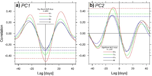
5°N-15°N and 20°W-0° (see map) for 1990-2010. The associated red noise spectrum with 95% confidence bounds is given by the black curves. The gray shading represents the 30-90-day band. ...25 Fig. 2.2 The 30-90-day 700 hPa PKE index lag correlated with (a) PC1 of the MJO
index and (b) PC2 of the MJO index. The black line includes JJAS for all 21 years. The blue line includes JJAS with at least 60 significant MJO days (14 years). The green line includes JJAS with at least 70 significant MJO days (ten years). The red line includes JJAS with at least 80 significant MJO days (six years). Dashed lines represent the 95% significant threshold for each subset. ...26 Fig. 2.3 Sample time series are shown for PC1 (black, dashed), PC2 (blue,
dot-dashed), and 30-90-day 700 hPa PKE (red, solid) indices for a boreal summer with strong MJO activity (1 May 2002 and 31 October 2002). Each index is normalized by its standard deviation. ...27 Fig. 2.4 Lead/Lag composites for a) Day -7 and b) Day 0 for ERA-Interim 400 hPa
30-90-day temperature anomalies. The shading interval is 0.1 K. Stippling represents 95% significance. ...28
Fig. 2.5 Lead/Lag composites of a) Day -7 and b) Day 0 for ERA-Interim 30-90-day 200-400 hPa thickness anomalies. The shading interval is 10 m. Stippling represents 95% significance. ...29 Fig. 2.6 Boreal summer power spectra for CLAUS TB averaged between
10°N-24°N and 16.5°E-27.5°E for 1989-2005. The associated red noise spectrum with 95% confidence bounds is given by the black curves. The gray shading represents the 30-90-day band. ...31 Fig. 2.7 Lead/Lag composites of 30-90-day TB anomalies averaged for day -2
through day +2 with respect to a 30-90-day TB index in the trigger region (marked by a black box). Composites are shown for a), significant positive 30-90-day TB events, and b) significant negative 30-90-day TB events. The shading interval is 0.6 K. Stippling represents 30-90-day TB anomalies that are significant with 95% confidence. ...32 Fig. 2.8 As in 2.6, except for ERA-Interim OLR from 1990-2010. ...33 Fig. 2.9 The correlation of the PKE index with negative ERA-Interim OLR
anomalies averaged in the trigger region. Negative lag days represent OLR leading PKE. ...34 Fig. 2.10 Lead/lag composites for positive PKE events in June-September
(1990-2010) are averaged between 10°N and 20°N to create a Hovmöller diagram of 30-90-day OLR anomalies. The shading interval is 0.5 W m-2. Stippling represents OLR30-90 anomalies that are significant with 95%
confidence. The thick vertical dashed line marks the longitudinal center for the PKE index region, and the thick horizontal dashed line marks Day 0...34 Fig. 2.11 As in 2.10, except for 700 hPa PKE30-90 anomalies composited for
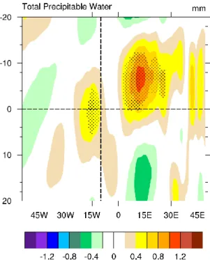
significant OLR events in East Africa. The latitude range is changed to 10°N and 15°N. ...35 Fig. 2.12 As in 2.6, except for ERA-Interim TPW from 1990-2010. ...36 Fig. 2.13 The correlation of negative Interim OLR anomalies with
ERA-Interim TPW anomalies, both averaged in the trigger region. Negative lag days represent TPW leading OLR. ...36 Fig. 2.14 The correlation of the PKE index with ERA-Interim TPW anomalies,
averaged in the trigger region. Negative lag days represent TPW leading PKE. ...37 Fig. 2.15 As in 2.10, except for TPW30-90 anomalies composites for significant West
Fig. 2.16 As in 2.10, except for PKE30-90 anomalies composites for significant East
African TPW30-90 events. ...38
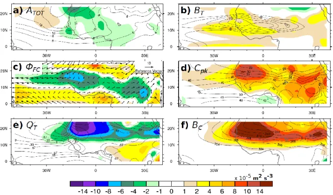
Fig. 2.17 The vertically integrated PKE and PAPE budget terms and supporting fields are averaged in boreal summer (June-September). All budget terms are shaded and use the same color bar. Shown: (a) PKE advection (ATOT) and 700 hPa PKE (contours; interval of 2 m2 s-2), (b) barotropic energy conversion (BT) and 650 hPa zonal wind (contours; interval of 1 m s-1 less than -7 m s-1), (c) geopotential flux convergence (ΦFC) and 850 hPa total wind (vectors), (d) baroclinic overturning (Cpk) and total precipitable water (contours; interval of 5 mm), (e) diabatic generation of PAPE (QT) and the mean apparent heating rate (contours; interval of 0.33 K day-1), and (f) baroclinic energy conversion (BC) and 850 hPa potential temperature (contours; interval of 2 K). ...40 Fig. 2.18 The vertical structure of the PKE and PAPE budget terms and supporting
fields are averaged between 10°W and 20°E during boreal summer (June-September). All budgets terms are shaded. Shown: (a) PKE advection (ATOT) and PKE (contours; interval of 2 m2 s-2), (b) barotropic energy conversion (BT) and zonal wind (contours; interval of 1 m s-1 less than -7 m s-1), (c) geopotential flux convergence (ΦFC) and total wind (vectors), (d) baroclinic overturning (Cpk) and total wind (vectors), (e) diabatic generation of PAPE (QT) and the apparent heating rate (contours; interval of 1 K day-1), and (f) baroclinic energy conversion (BC) and potential temperature (contours; : interval of 2.5 K; : interval of 5 K). ...41 Fig. 2.19 As in Fig.2.18, except for the vertical structure of (a) the PKE residual
term (D) and (b) the PAPE residual term (R). ...44 Fig. 2.20 As in Fig. 2.17, except for boreal summer mean CFSR data (2000-2010)...45 Fig. 2.21 Lead/lag composites are averaged between 10°N and 15°N to create
Hovmöller diagrams. Shown: 30-90-day 700 hPa PKE anomalies (shading) and vertically averaged 30-90-day PKE tendency (contours) for June-September composited for significant events in a 30-90-day 700 hPa PKE index. The shading interval is 0.5 m2 s-2. The contour interval is 4x10⁻⁷ m2 s-3. Stippling represents PKE anomalies that are significant with 95% confidence. The thick vertical dashed line marks the longitudinal center for the PKE index region. The thick horizontal dashed line marks Day 0. ...47 Fig. 2.22 Lead/lag maps of 30-90-day 700 hPa PKE anomalies (shading) and
vertically averaged 30-90-day PKE tendency (contours) for June-September composited for significant events in a 30-90-day 700 hPa PKE index. Shown: (a) day -10 and (b) day 0. The shading interval is 0.4 m2 s-2.
The contour interval is 4x10⁻⁷ m2 s-3. Stippling represents PKE anomalies that are significant with 95% confidence. Coastlines are represented by a gray contour. ...48 Fig. 2.23 As in Fig. 2.21, except for vertically averaged, 30-90-day PKE creation
terms south of the AEJ (7.5°N – 12.5°N). Shown: (a) barotropic energy conversion, (b) baroclinic overturning, (c) baroclinic energy conversion, and (d) PAPE generation by diabatic heating. Lead/lag composites are averaged between 7.5°N and 12.5°N to create Hovmöller diagrams. The shading interval is 2x10⁻⁶ m2 s-3. ...50 Fig. 2.24 As in Fig. 2.21, except for vertically averaged, 30-90-day PKE creation
terms north of the AEJ (12.5°N – 17.5°N). Shown: (a) barotropic energy conversion, (b) baroclinic overturning, (c) baroclinic energy conversion, and (d) PAPE generation by diabatic heating. Lead/lag composites are averaged between 12.5°N and 17.5°N to create Hovmöller diagrams. The shading interval is 2x10⁻⁶ m2 s-3. If necessary, contours represent levels outside of the shading limits with an interval of 4x10⁻⁶ m2 s-3. ...51 Fig. 2.25 As in Fig. 2.22, except for vertically averaged, 30-90-day PKE creation
terms on day -10. Shown: (a) barotropic energy conversion, (b) baroclinic overturning, (c) baroclinic energy conversion, and (d) PAPE generation by diabatic heating. The shading interval is 2x10⁻⁶ m2 s-3. If necessary, contours represent levels outside of the shading limits with an interval of 4x10⁻⁶ m2 s-3. Coastlines are represented by a gray contour. ...52 Fig. 2.26 As in Fig. 2.22, except for vertically averaged, 30-90-day PKE creation
terms on day 0. Shown: (a) barotropic energy conversion, (b) baroclinic overturning, (c) baroclinic energy conversion, and (d) PAPE generation by diabatic heating. If necessary, contours represent levels outside of the shading limits with an interval of 4x10⁻⁶ m2 s-3. Coastlines are represented by a gray contour. ...52 Fig. 2.27 Day 0 regression of Q1’ (shading) and T’ (contours) against 700 hPa eddy
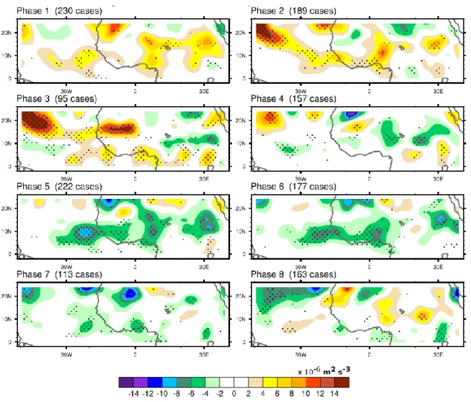
vorticity averaged in the shown black box. The shading interval is 0.04 K day-1. The contour interval is 0.02 K. Stippling represents shading that is 95% significant. The gray contour represents that African coastline. ...55 Fig. 2.28 MJO phase composites for 30-90-day 700 hPa PKE anomalies (shading)
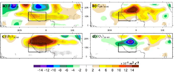
and vertically averaged 30-90-day PKE tendency (contours) for June-September. The shading interval is 0.3 m2 s-2. The contour interval is 4x10⁻⁷ m2 s-3. Stippling represents PKE anomalies that are significant with 95% confidence. Coastlines are represented by a gray contour...58 Fig. 2.29 As in Fig. 2.28, except for vertically-averaged 30-90-day BT anomalies.
Fig. 2.30 As in Fig. 2.28, except for vertically-averaged 30-90-day Cpk anomalies. The shading interval is 2x10⁻⁶ m2 s-3...61 Fig. 2.31 As in Fig. 2.28, except for vertically-averaged 30-90-day BC anomalies.
The shading interval is 2x10⁻⁶ m2 s-3...62 Fig. 2.32 As in Fig. 2.28, except for vertically-averaged 30-90-day QT anomalies.
The shading interval is 2x10⁻⁶ m2 s-3...64 Fig. 2.33 As in Fig. 2.22, except for: (a) 30-90-day 700 hPa meridional zonal wind
gradient anomalies (shading) and 30-90-day 700 hPa zonal wind ≤ -7 m s-1 (contours) on day -10, (b) (a) on day 0, (c) 30-90-day 850 hPa meridional temperature gradient anomalies on day -10, and (d) (c) on day 0. Please note that the shading interval is 2 x 10⁻⁷ s-1 in (a), (c) and 1 x 10⁻⁷ K m-1 in (b), (d). The contour interval is 1 m s-1 in (a), (c). Coastlines are represented by a gray contour. ...66 Fig. 2.34 As in Fig. 2.21, except for: (a) 30-90-day 700 hPa barotropic energy
conversion anomalies, (b) 30-90-day 850 hPa baroclinic energy conversion anomalies north of the AEJ, (c) BT1 anomalies, (d) BC1 anomalies, (e) BT2 anomalies, and (f) BC2 anomalies. (a), (c), and (e) have a shading interval of 2 x 10⁻⁶ m2 s-3 and are analyzed south of the AEJ. (b), (d), and (f) have a shading interval of 1 x 10⁻⁵ m2 s-3 and are analyzed north of the AEJ. If necessary, contours extend above/below the shading limits with an interval of 2 x 10⁻⁶ m2 s-3...67 Fig. 2.35 As in Fig. 2.21, except for: (a) 30-90-day 700 hPa PKE anomalies
associated with positive PKE events over the East Atlantic and (b) 30-90-day 700 hPa PKE anomalies associated with negative PKE events over the East Atlantic. Hovmollers are averaged between 10°N and 15°N. Tropical cyclogenesis events (stars) are from the Revised Hurricane Database (HURDAT2). The shading interval is 0.3 m2 s-2. ...70 Fig. 2.36 MJO phase composites for ERA-Interim 30-90-day 700 hPa PKE
anomalies Tropical cyclogenesis events (stars) are from the Revised
Hurricane Database (HURDAT2). The shading interval is 0.3 m2 s-2. ...71 Fig. 2.37 MJO phase composites for ERA-Interim 30-90-day OLR anomalies.
Tropical cyclogenesis events (stars) are from the Revised Hurricane Database (HURDAT2). The shading interval is 0.5 W m-2. ...72 Fig. 3.1 A schematic showing how the root system of modeled vegetation
penetrates into different layers for NCEP soil data (left) and ERA-Interim soil data (right). ...83
Fig. 3.2 Boreal summer mean (June-August) precipitation maps for a) TRMM 3B42, b) WSM6 microphysics and RUC land surface model, c) WSM6 microphysics and Noah land surface model, d) Thompson microphysics and RUC land surface model, and e) Thompson microphysics and NOAH land surface model. The shading interval is 0.5 mm day-1. All plots are on the same scale. ...86 Fig. 3.3 Boreal summer mean (June-August) 650 hPa zonal wind maps for a)
ERA-Interim, b) WSM6 microphysics and RUC land surface model, c) WSM6 microphysics and Noah land surface model, d) Thompson microphysics and RUC land surface model, and e) Thompson microphysics and NOAH land surface model.. The shading interval is 2 m s-1. All plots are on the same scale. ...86 Fig. 3.4 As in Fig. 3.3, except for zonal wind cross-sections averaged between
20°W and 0°E. The shading interval is 2 m s-1. All plots are on the same scale...87 Fig. 3.5 As in Fig. 3.3, except for zonal wind cross-sections averaged between 0°E
and 20°E. The shading interval is 2 m s-1. All plots are on the same scale. ...88 Fig. 3.6 Hovmöller diagrams of 700 hPa relative vorticity for a) ERA-Interim, b)
WSM6 microphysics and RUC land surface model, c) WSM6 microphysics and NOAH land surface model, d) Thompson microphysics and RUC land surface model, and e) Thompson microphysics and NOAH land surface model.. The shading interval is 0.5x10⁻⁵ m s-1. All plots are on the same scale. ...89 Fig. 3.7 Boreal summer mean (June-August) precipitation maps for a) TRMM
3B42, b) WRF-ARW, and c) WRF-NMM. The shading interval is 0.5 mm day-1...92 Fig. 3.8 Boreal summer mean (June-August) 650 hPa zonal wind maps for a)
ERA-Interim, b) WRF-ARW, and c) WRF-NMM. The shading interval is 2 m s-1. ...93 Fig. 3.9 Boreal summer mean (June-August) zonal wind cross-sections for a)
ERA-Interim, b) WRF-ARW, and c) WRF-NMM. Plots are averaged between 20°W and 0°E. The shading interval is 2 m s-1...93 Fig. 3.10 Boreal summer mean (June-August) zonal wind cross-sections for a)
ERA-Interim, b) WRF-ARW, and c) WRF-NMM. Plots are averaged between 0°E and 20°E. The shading interval is 2 m s-1. ...93 Fig. 3.11 Hovmöller diagrams of 700 hPa relative vorticity for a) ERA-Interim, b)
15°N. The shading interval is 0.5x10⁻⁵ m s-1. The time axis is positive
going down...95
Fig. 3.12 Boreal summer (June-August) meridional wind regressed against eddy 700 hPa vorticity for a) ERA-Interim, b) WRF-ARW, and c) WRF-NMM. In a), eddy vorticity at measured at the star. In b) and c), eddy vorticity is averaged in the black box. The shading interval is 0.2 m s-1. ...95
Fig. 3.13 As in Fig. 3.11, except for 700 hPa PKE. The scales vary for each plot. ...95
Fig. 4.1 Wavenumber-frequency filtering of the boundary conditions for the three proposed WRF experiments. In a), no filtering is applied. In b), all 30-90-day variability is removed. In c), only eastward-propagating wavenumbers 0 to 10 are removed from the 30-90-day band. Filtered parts of the wavenumber-frequency domain are represented by blue shading. Figure is adapted from Wheeler and Kiladis (1999). ...101
Fig 4.2 Boreal summer mean precipitation for three WRF-ARW experiments: a) C1, b) S1, and c) S2. The shading interval is 1 mm day-1. ...103
Fig. 4.3 Boreal summer mean 650 hPa zonal wind for three WRF-ARW experiments: a) C1, b) S1, and c) S2. The shading interval is 2 m s-1. 650 hPa total wind vectors are overlaid. ...104
Fig 4.4 Boreal summer mean zonal wind averaged between 10°W and 20°E for three WRF-ARW experiments: a) C1, b) S1, and c) S2. The shading interval is 2 m s-1. ...104
Fig 4.5 Eddy 700 hPa meridional wind regressed against eddy 700 hPa vorticity averaged in the black box for three WRF-ARW experiments: a) C1, b) S1, and c) S2. The shading interval is 0.4 m s-1. Stippling represents values that exceed the 95% confidence threshold. ...104
Fig 4.6 As in Fig. 2.17, except for C1. ...106
Fig 4.7 As in Fig. 2.18, except for C1. ...107
Fig 4.8 As in Fig. 2.17, except for S1. ...109
Fig 4.9 As in Fig. 2.18, except for S1. ...110
Fig 4.10 As in Fig. 2.17, except for S2. ...111
Fig 4.12 Boreal summer 30-90-day variance maps of 700 hPa PKE for three
WRF-ARW experiments (C1, S1, S2). ...114 Fig 4.13 Boreal summer power spectra for 700 hPa PKE for different WRF
simulations from 2001 to 2010 for: a) C1), b) S1, and c) S2. Maps show the area where spectra are computed. The associated red noise spectrum with 95% confidence bounds is given by the black curves. The gray shading represents the 30-90-day band. ...115 Fig 4.14 Correlation coefficients for West African 700 hPa PKE indices for
observations (ERA-I) and three WRF-ARW experiments (C1, S1, S2). Correlations are performed for June-Sept from 2001-2010.. ...116 Fig 4.15 As in Fig. 2.21, except for the three WRF-ARW experiments averaged
over different latitudes: a) C1 (10°N-20°N), b) S1 (11°N-21°N), and c) S2 (13°N-23°N). The shading interval is 1 m2 s-2. Stippling represents significance at the 95% confidence level. ...119 Fig 4.16 As in Fig. 2.22, except for the three WRFARW experiments: a) C1 day
-10, b) S1 day --10, c) S2 day --10, d), C1 day 0, e) S1 day 0, and f) S2 day 0. The shading interval is 1 m2 s-2. Stippling represents significance at the 95% confidence level. ...119 Fig 4.17 As in Fig. 2.21, except for vertically averaged, 30-90-day PKE creation
terms south of the AEJ (10°N – 15°N) in the C1 simulation. Shown: (a) barotropic energy conversion, (b) baroclinic overturning, (c) baroclinic energy conversion, and (d) PAPE generation by diabatic heating. Lead/lag composites are averaged between 10°N and 15°N to create Hovmöller diagrams. The shading interval is 2x10⁻⁶ m2 s-3. Contours represent levels outside of the shading limits with an interval of 4x10⁻⁶ m2 s-3. ...121 Fig 4.18 As in Fig. 2.21, except for vertically averaged, 30-90-day PKE creation
terms north of the AEJ (15°N – 20°N) in the C1 simulation. Shown: (a) barotropic energy conversion, (b) baroclinic overturning, (c) baroclinic energy conversion, and (d) PAPE generation by diabatic heating. Lead/lag composites are averaged between 15°N and 20°N to create Hovmöller diagrams. The shading interval is 2x10⁻⁶ m2 s-3. Contours represent levels outside of the shading limits with an interval of 4x10⁻⁶ m2 s-3. ...122 Fig 4.19 As in Fig. 2.22, except for vertically averaged, 30-90-day PKE creation
terms on day -10 in the C1 simulation. Shown: (a) barotropic energy conversion, (b) baroclinic overturning, (c) baroclinic energy conversion, and (d) PAPE generation by diabatic heating. The shading interval is 2x10
-6 m2 s-3. Contours represent levels outside of the shading limits with an
Fig 4.20 As in Fig. 2.22, except for vertically averaged, 30-90-day PKE creation terms on day 0 in the C1 simulation. Shown: (a) barotropic energy conversion, (b) baroclinic overturning, (c) baroclinic energy conversion, and (d) PAPE generation by diabatic heating. The shading interval is 2x10
-6 m2 s-3. Contours represent levels outside of the shading limits with an
interval of 4x10⁻⁶ m2 s-3...123 Fig 4.21 As in Fig. 2.21, except for vertically averaged, 30-90-day PKE creation
terms south of the AEJ (13°N – 18°N) in the S1 simulation. Shown: (a) barotropic energy conversion, (b) baroclinic overturning, (c) baroclinic energy conversion, and (d) PAPE generation by diabatic heating. Lead/lag composites are averaged between 13°N and 18°N to create Hovmöller diagrams. The shading interval is 2x10⁻⁶ m2 s-3. Contours represent levels outside of the shading limits with an interval of 4x10⁻⁶ m2 s-3. ...126 Fig 4.22 As in Fig. 2.21, except for vertically averaged, 30-90-day PKE creation
terms north of the AEJ (18°N – 23°N) in the S1 simulation. Shown: (a) barotropic energy conversion, (b) baroclinic overturning, (c) baroclinic energy conversion, and (d) PAPE generation by diabatic heating. Lead/lag composites are averaged between 18°N and 23°N to create Hovmöller diagrams. The shading interval is 2x10⁻⁶ m2 s-3. Contours represent levels outside of the shading limits with an interval of 4x10⁻⁶ m2 s-3. ...127 Fig 4.23 As in Fig. 2.22, except for vertically averaged, 30-90-day PKE creation
terms on day -10 in the S1 simulation. Shown: (a) barotropic energy conversion, (b) baroclinic overturning, (c) baroclinic energy conversion, and (d) PAPE generation by diabatic heating. The shading interval is 2x10
-6 m2 s-3. ...128
Fig 4.24 As in Fig. 2.22, except for vertically averaged, 30-90-day PKE creation terms on day 0 in the S1 simulation. Shown: (a) barotropic energy conversion, (b) baroclinic overturning, (c) baroclinic energy conversion, and (d) PAPE generation by diabatic heating. The shading interval is 2x10
-6 m2 s-3. Contours represent levels outside of the shading limits with an
interval of 4x10⁻⁶ m2 s-3...128 Fig 4.25 As in Fig. 2.28, except for 700 hPa 30-90-day PKE anomalies in the C1
simulation. The shading interval is 0.5 m2 s-2. ...132 Fig 4.26 As in Fig. 2.28, except for vertically-averaged 30-90-day BT anomalies in
the C1 simulation. The shading interval is 2x10⁻⁶ m2 s-3. ...133 Fig 4.27 As in Fig. 2.28, except for vertically-averaged 30-90-day BC anomalies in
Fig 4.28 As in Fig. 2.28, except for 700 hPa 30-90-day PKE anomalies in the S1 simulation. The shading interval is 0.5 m2 s-2. ...135 Fig 4.29 As in Fig. 2.21, except for 30-90-day 650 hPa zonal wind anomalies from
three WRF-ARW experiments averaged over different latitudes: a) C1 (12.5°N-17.5°N), b) S1 (15.5°N-20.5°N), and c) S2 (18°N-23°N). The shading interval is 0.3 m s-1. Stippling represents significance at the 95% confidence level. ...137 Fig 4.30 As in Fig. 2.22, except for 30-90-day 650 hPa zonal wind anomalies from
three WRFARW experiments: a) C1 day 10, b) S1 day 10, c) S2 day -10, d), C1 day 0, e) S1 day 0, and f) S2 day 0. The shading interval is 0.3 m s-1. Stippling represents significance at the 95% confidence level. ...137 Fig 4.31 As in Fig. 2.21, except for 30-90-day 400 hPa temperature anomalies from
three WRF-ARW experiments averaged between 22.5°N-27.5°N: a) C1, b) S1, and c) S2. The shading interval is 0.1 K. Stippling represents significance at the 95% confidence level. ...139 Fig 4.32 As in Fig. 2.22, except for 30-90-day 400 hPa temperature anomalies from
three WRFARW experiments: a) C1 day 10, b) S1 day 10, c) S2 day -10, d), C1 day 0, e) S1 day 0, and f) S2 day 0. The shading interval is 0.3 m s-1. Stippling represents significance at the 95% confidence level. ...139 Fig 4.33 As in Fig. 2.21, vertically-integrated 30-90-day anomalies of the following
moisture budget terms from the C1 simulation averaged over different latitudes: a) C1 (12.5°N-17.5°N), b) S1 (15.5°N-20.5°N), and c) S2 (18°N-23°N). The shading interval is 0.1 mm day-1. Stippling represents significance at the 95% confidence level. ...141 Fig 4.34 As in Fig. 2.22, except for vertically-integrated 30-90-day anomalies of
the following moisture budget terms from the C1 simulation: a) moisture tendency day -10, b) meridional moisture advection day -10, c) precipitation day -10, d), moisture tendency day 0, e) meridional moisture advection day 0, and f) precipitation day 0. The shading interval is 0.1 mm day-1. Stippling represents significance at the 95% confidence level. ...141 Fig 4.35 As in Fig. 2.28, except for vertically-integrated 30-90-day moisture
tendency anomalies in the C1 simulation. The shading interval is 0.5 mm day-1...143
LIST OF TABLES
Table 3.1 Comparison of attributes within the WRF-ARW and WRF-NMM dynamical cores. ...78 Table 3.2 Comparsison of the parameterizations used in the ARW and
WRF-NMM dynamical cores. ...91 Table 4.1 Correlation coefficients for West African 700 hPa PKE indices for
observations (ERA-I) and three WRF-ARW experiments (C1, S1, S2). Correlations are performed for June-Sept from 2001-2010. ...117
CHAPTER 1 Introduction
1.1 Improving Prediction of African Easterly Wave Activity
African easterly waves (AEWs; see Section 1.2) are synoptic-scale disturbances that exhibit significant variations on intraseasonal timescales (i.e., 30-90-day) in West Africa (Leroux and Hall 2009; Alaka 2010; Alaka and Maloney 2012). Simply examining visible satellite imagery from the Moderate-resolution Imaging Spectroradiometer (MODIS) over the course of a boreal summer reveals several active and quiet periods of AEW activity (Fig. 1.1). For example, the period from August 15-30, 2012 featured several successive AEWs that developed into Atlantic tropical cyclones at some point in the basin: Hurricane Gordon, Tropical Storm Helene, Hurricane Isaac, Tropical Storm Joyce, Hurricane Kirk, and Hurricane Leslie. In September, 2012, which is the climatological height of the Atlantic hurricane season, only one Atlantic system formed from an AEW (Hurricane Nadine). Based on a wave tracking algorithm presented in Wang et al. (2012), AEW activity was stronger in August, 2012 than in September. Thus, an oscillation in AEW activity emerging from the West African coast could directly impact tropical cyclogenesis in the Atlantic. What factors contribute to this intraseasonal oscillation of AEW activity? Further, is 30-90-day AEW activity internally or externally forced? Given the dominance of the Madden-Julian oscillation (MJO; see Section 1.4) in the tropics on 30-90-day time scales, it is the leading candidate for an externally-forced modulation of AEW activity. If the slowly-evolving MJO and West African AEW activity are indeed highly-correlated, then the prediction of these synoptic-scale eddies would improve considerably. Models such as the monthly European Centre for Medium-Range Weather Forecasts (ECMWF) Ensemble Prediction System (EPS) exhibit strong sensitivity of Atlantic tropical cyclone activity to MJO
phasing and amplitude (Vitart 2009; Belanger et al. 2010), which has been partly attributed to the ISV of AEWs. The MJO is predicted with skill 3-4 weeks in advance (Waliser et al. 2006; Vitart and Molteni 2010), which could lead to a significant improvement in forecast skill for AEWs.
However, the West African monsoon (WAM) might also be influenced by several other atmospheric phenomena that project onto the 30-90-day band. In particular, the North Atlantic oscillation (NAO; Walker 1924) and the qausi-biweekly zonal dipole (QBZD; Mounier et al. 2008). might have a strong influence on intraseasonal activity in West Africa. Additionally, intraseasonal variability in this region could be internally-forced, associated with active/break cycles in the monsoon, movement of the Saharan heat low, and/or complex topography.
Fig. 1.1 MODIS satellite imagery from Aug. 20, 2012 patched together to show successive African easterly waves (marked by letters) that developed into Atlantic tropical cyclones. “G” stands for Gordon. “I” stands for Isaac. “J” stands for Joyce. “K” stands for Kirk. Image created in Google Earth.
Increasing the complexity, WAM and Saharan heat low variability could be modulated by external phenomena, providing an indirect pathway to AEW modulation.
Improving AEW forecasts is important for two primary reasons: 1) the rainfall associated with AEWs is vital to Sahelian agriculturalists (Sultan et al. 2005), and 2) AEWs seed Atlantic and eastern Pacific tropical cyclones (e.g., Hopsch et al. 2007), which cause significant damage to North American, Central American, and Caribbean communities (Avila 1991; Avila and Pasch 1992; Landsea et al. 1999; Pielke et al. 2008). The improvement of medium-range AEW forecasts in West Africa based on trends in 30-90-day anomalies is a fruitful avenue to explore due to the dominance of the quasi-predictable Madden-Julian oscillation in this frequency band. Such improved forecasts could increase lead time to distribute forecasts to self-sustaining Sahelian farmers and could allow the National Hurricane Center (NHC) to focus more resources on the East Atlantic when 30-90-day AEW activity trends upward. Given the relationship between the MJO and AEW precursors in East Africa (Alaka and Maloney 2012; see Section 1.5), this region will be studied as an initiation region for increases in downstream 30-90-day AEW activity. In this study, the growth, maintenance, and decay of AEWs on intraseasonal (i.e., 30-90-day) time scales are scrutinized using perturbation energy and moisture budgets. Thus, the evolution of 30-90-day AEW activity will be linked to dynamical and diabatic sources of kinetic energy.
1.2 African Easterly Waves: An Overview
African easterly waves (AEWs) are synoptic-scale eddies that initiate and grow via energy conversions over tropical North Africa during boreal summer (Carlson 1969a,b; Burpee 1972, 1974; Norquist et al. 1977; Reed et al. 1977). These eddies have wavelengths of 3000-4000 km (Kiladis et al. 2006) and are characterized by a 2.5-6-day regime that is symmetric
about the African easterly jet (AEJ; Diedhiou et al. 1999; Pytharoulis and Thorncroft 1999). The eddies to the south of the AEJ (i.e., AEWs) are typically characterized by strong fluctuations in deep convection and vorticity signatures at 700 hPa, while the eddies north of the AEJ are typically dry, are located near 900 hPa, and are generally unimportant for tropical cyclogenesis (Thorncroft and Hodges 2001; Zawislak and Zipser 2010). The northern and southern eddy tracks converge into a single track in the eastern Atlantic just north of the AEJ (Reed et al. 1988). Several studies have identified a 6-9-day regime that is asymmetric about the AEJ, but these disturbances appear to be dynamically different from AEWs (Diedhiou et al. 1998, 1999; Wu et al. 2013).
AEWs generally initiate somewhere east of 10°E in association with convection and topography (Carlson 1969a,b). Recent studies have focused on upstream convective disturbances between the Darfur Mountains (15°N, 23°E) and Ethiopian Highlands (10°N, 25°E) that grow along the AEJ into mature AEWs (Hall et al. 2006; Kiladis et al. 2006; Mekonnen et al. 2006; Thorncroft et al. 2008; Leroux and Hall 2009). The Cameroon highlands (8°N, 10°E) and Fouta Djallon highlands (10°N, 10°W) may be important for spawning convection after AEWs have already developed and propagated downstream. (Thorncroft et al. 2008) contended that AEWs are initiated by a localized forcing in the form of upstream latent heating associated with topography, which is plausible given that upstream latent heating strengthens the meridional potential vorticity (PV) gradient associated with the WAM and provides a more favorable environment for AEW growth (Schubert et al. 1991). An influx of PV into this region from the midlatitudes implies that the extratropics could force AEW initiation also.
AEW characteristics evolve as these disturbances propagate to the west. For example, the phase speed of AEWs decreases from ~12 m s-1 east of Greenwich to 8.5 m s-1 over the central
Atlantic. Kiladis et al. (2006) found that the outgoing longwave radiation (OLR) signal propagates slightly slower than meridional wind and vorticity fields. In fact, convection tends to be on the west side of the wave axis while over land and on the east side of the wave axis over the East Atlantic (Kiladis et al. 2006). The wave axis appears to catch up to the convection approximately at the Greenwich Meridian. Kiladis et al. (2006) found that the meridional and zonal extents of AEWs are much greater than previously suggested. Meridionally, AEWs may extend from 20°S to 40°N, a huge expanse that opens up the possibility for interaction with the boreal midlatitudes. Analysis of the meridional wind at 10°N reveals a first baroclinic structure, with westward tilted wind maxima below 300 hPa and opposing meridional flow above 300 hPa (Reed et al. 1977; Kiladis et al. 2006). Additionally, National Centers for Environmental Prediction (NCEP) reanalysis and observations of the waves during the Global Atmospheric Research Program (GARP) Atlantic Tropical Experiment (GATE) field campaign provide evidence for a dynamical contraction of AEW zonal wavelengths as they propagate into the East Atlantic (Diediou et al. 1999; Reed et al. 1977). Due to a coupling with deep convection, AEWs feature a vertical structure that extends to the tropopause south of the AEJ. Kiladis et al. (2006) utilize reanalysis to show that the 200 hPa circulation is of the opposite sense to the low-level circulation and slightly displaced to the east. AEWs typically exhibit similar scale and structure as Pacific easterly waves (Reed and Recker 1971), although their generation mechanisms likely differ.
The growth, maintenance, and decay of AEWs are governed by energy conversions that alter the local kinetic energy of the disturbance (Norquist et al. 1977). These energy conversions are crucial to understanding the lifecycle of AEWs on different timescales. Barotropic and baroclinic energy conversions have been the focus of several studies (e.g., Norquist et al. 1977;
Thorncroft and Hoskins 1994a,b), since a reversal in the meridional gradient of PV satisfies the Charney-Stern necessary condition for instability (Charney and Stern 1962), which allows AEWs to grow via a mixed barotropic/baroclinic instability mechanism for about 50° of longitude (Dickinson and Molinari 2000). However, better observations (i.e., the African Multidisciplinary Monsoon Analyses, or AMMA, campaign in 2006) and finer-resolution modeling has increased confidence that diabatic heating within deep convection is an important driver of AEW growth. See Section 2.1 for a more detailed look into the history of research on AEW energetics.
1.3 The West African Monsoon
The West African monsoon (WAM) is a thermally-driven circulation that sets up due to the strong temperature gradient between the Sahara Desert and the Gulf of Guinea (Alaka 2010). The West African monsoon is a complex system, with several jets and circulations tightly fit into a ~4000 km stretch from south of the equator to Europe (Fig. 1.2). The intertropical discontinuity (ITD) is a surface front that marks the convergence of moist southwesterly monsoon flow (shaded red in Fig. 1.2) with dry northeasterly flow that resembles a weaker version of the winter Harmattan winds (shaded blue in Fig. 1.2; Sultan and Janicot 2003). This convergence, which is visible even at 850 hPa (near 20°N in Fig. 1.3a), fuels the Saharan heat low (~20°N) and pumps air upward in a dry adiabatic layer that extends to nearly 600 hPa (see Fig. 2.18f). This dry adiabatic layer over the Sahara Desert results in a nearly-constant potential temperature (θ) in the lower-troposphere. The reduced potential temperature gradient with respect to pressure in this region is reflected by low Ertel PV (Hoskins et al. 1985), which reverses the sign of the meridional PV gradient and satisfies the necessary condition for combined barotropic-baroclinic instability, as outlined in Charney and Stern (1962) and revisited by Eliassen (1983). It is
Fig. 1.2 Schematic of the West African monsoon system as viewed from the West adapted from Lafore et al. (2010). “TEJ” in the yellow tube stands for AEJ.
important to note that the Charney-Stern condition for instability is not sufficient, which implies that barotropic and baroclinic energy conversions do not automatically exist in the presence of a meridional PV gradient reversal. The nature of this barotropic-baroclinic instability and its impact of AEW activity on intraseasonal timescales is a focal point of this dissertation.
The African easterly jet (AEJ) is the WAM feature that is most relevant to African easterly waves (AEWs), given the associated barotropic and baroclinic instabilities arising from a reversal in the meridional PV gradient (Charney and Stern 1962). Positioned zonally across North Africa near 15°N, the AEJ, which resides near 650 hPa, is in thermal wind balance with the aforementioned meridional temperature gradient in the region. With maximum easterly velocities over 12 m s-1 in the boreal mean, the AEJ induces significant cyclonic shear, which creates energy for AEWs through barotropic energy conversion (see Section 2.3). Although the AEJ appears as if it were a constant river of air in boreal mean plots (Fig. 1.3b), the reality is that
Fig. 1.3 June-September average plots for zonal wind (shading) and total wind (vectors) from 21 years (1990-2010) of ECMWF ERA-Interim data. Winds are plotted at a) 850 hPa and b) 650 hPa.
the AEJ is quite wavy, with surges of easterly flow helping to roll up 700 hPa vortices associated with AEWs and more quiescent periods with broader, weaker flow.
The tropical easterly jet (TEJ) is a feature near the tropopause over land that dips down into the upper troposphere over the equatorial Atlantic Ocean. In general, the tropical easterly jet does not significantly impact AEW activity. The subtropical jet is located at 200 hPa near 30°N. The subtropical jet might interact with AEW activity through jet breakdowns that result in injections of midlatitude PV into tropical Africa. In fact, boreal summers with stronger subtropical jet breakdowns, which might be linked to the El Nino southern oscillation, feature fewer AEWs propagating into the East Atlantic (personal correspondence with Dr. Thomas Galarneau).
Given the complexity of the WAM, it is imperative that regional climate models reproduce key features of this system in order to reliably compare model output to observations (e.g., reanalyses). Neither the tropical easterly jet nor the subtropical jet have been known to
b) a)
interact much with AEW activity, so the reproduction of these features within a regional modeling framework will not be a focus.
1.4 The Madden-Julian Oscillation
The Madden-Julian oscillation (MJO) is the dominant mode of intraseasonal (i.e., 30-90-day) variability in the tropics that dominates zonal wavenumbers one to three (Zhang 2005). It was first discovered by Roland Madden and Paul Julian, for whom the phenomenon is named, when they noticed a periodic reversal in the winds every 40-50 days in rawinsonde data from several West Pacific locations (Madden and Julian 1971). When they later expanded their coverage to a more global perspective, they were able to piece together a life cycle for the MJO, with eight phases detailing the state of convection and the position of large-scale zonal circulation cells (Madden and Julian 1972). Overall, the MJO is coupled to convection from its initiation in the Indian Ocean to the International Dateline. Although the main convective envelope of the MJO erodes by the Dateline, the large scale circulation response is global. Thus, the large scale circulation associated with the MJO can produce secondary convection centers in the East Pacific, Atlantic, and Africa (e.g., Hendon and Salby 1994). While the main MJO convective signal is over the Indo-Pacific warm pool, the MJO propagates at ~5 m s-1. Once decoupled from convection east of the Dateline, the MJO signal speeds up to a velocity of 10-15 m s-1 (Zhang 2005), often times completing a zonal circuit and enhancing the aforementioned secondary convection centers along the way (e.g., Maloney and Esbensen 2003; Matthews 2004, 2008). In the Indian and West Pacific Oceans, the MJO envelope guides a non-uniform precipitation field that varies due to mesoscale effects.
It should be noted that the initiation and propagation mechanisms of the MJO are still up for debate. However, a recent study by Johnson and Ciesielski (2013) utilized observations from the Dynamics of the MJO (DYNAMO; Yoneyama et al. 2013; Zhang et al. 2013) field campaign to deduce that a gradual moistening of the troposphere precedes an MJO event. Moisture mode theory has emerged as a promising theory to explain the eastward propagation and destabilization of the MJO (e.g., Fuchs and Raymond 2007; Sobel and Maloney 2013). Specifically, the term “moisture mode” describes a disturbance that exists under weak temperature gradients and is regulated by the processes controlling the tropical moisture field (Sobel et al. 2001; Sugiyama 2009a,b). Hopefully, these advances will translate into improved simulations of the MJO in global models.
The MJO circulation responds to diabatic heating induced by deep convection on the equator, which produces a response that is similar to the idealized simulations in the Gill model (Heckley and Gill 1984). Consequently, the equatorial wave response includes forced equatorial Kelvin waves, which propagate ahead of the MJO heating to the east, and equatorial Rossby waves, which take the form of two low pressure systems that straddle the equator and propagate to the west (Matsuno 1966). This Kelvin-Rossby wave response is attached to the MJO heating and is dragged to the east. However, the Kelvin-Rossby response appears to grow in the zonal direction with time even with realistic damping (Heckley and Gill 1984). The MJO is also associated with transient convectively coupled Kelvin waves, which travel faster than the MJO convective envelope and tend to enhance convection in all parts of their world with their passage (Straub and Kiladis 2002, 2003; Roundy 2008; Ventrice et al. 2012; Ventrice and Thorncroft 2013).
Kelvin waves and the MJO explain about the same amount of convective variance (Wheeler and Kiladis 1999), although the former occur at a much wider range of spatial scales and are more meridionally confined to the equator. The Kelvin wave is a symmetric solution to the shallow water equations, and may be coupled or uncoupled with convection (Fig. 1.4b). Convectively coupled Kelvin waves have been shown to enhance convection along the equator with their passage, especially with existing disturbances such as a tropical cyclone (Straub and Kiladis 2002; Ventrice et al. 2012; Ventrice and Thorncroft 2013). Convectively coupled Kelvin waves propagate to the east at 10-25 m s-1, although uncoupled Kelvin waves propagate much faster (Wheeler et al. 2000). An equatorial Rossby wave is a westward-propagating symmetric response to the shallow water equations, with two low pressure gyres situated on either side of the equator (Fig. 1.4a; Matsuno 1966). Given the cyclonic circulation associated with equatiorial Rossby gyres, westerly wind bursts are commonly associated with equatorial Rossby waves. Generally, the poleward flow around each gyre is rising and convectively active, while the equatorward flow subsides and is mostly devoid of convection (Wheeler and Kiladis 1999).
Fig. 1.4 a) Structure of an equatorial Rossby wave from Fig. 4c in Matsuno (1966). b) Structure of an
In addition, MJO activity has been linked to worldwide tropical cyclone activity (Maloney and Hartmann 2000a,b, 2001a; Hall et al. 2001; Ventrice et al. 2011; Slade and Maloney 2013). The East Pacific exhibits significant intraseasonal variability, which may be forced partly by local dynamics and partly by the MJO signal propagating across the equatorial Pacific Ocean (Maloney and Hartmann 2000a; Maloney and Esbensen 2003; Rydbeck et al. 2013; Rydbeck and Maloney 2014). Recent studies have linked the MJO with the NAO, which has implications for the storm track and intensity of midlatitude systems on the eastern United States and Europe (Cassou 2008; Lin et al. 2009). The MJO has even been linked with severe tornado outbreaks in the United States (Thompson and Roundy 2013). Finally, as part of the foundation for this study, the MJO has been linked with the West African monsoon in previous studies (See Section 1.5).
1.5 The Influence of the Madden-Julian Oscillation on African Easterly Waves
Previous studies have documented the intraseasonal variability (ISV) of AEWs and the potential mechanisms that drive it. North African ISV may be attributed to large-scale phenomena like the MJO (Matthews 2004; Maloney and Shaman 2008; Janicot et al. 2009; Ventrice et al. 2011; Alaka Jr. and Maloney 2012) or to regional processes like land-surface interactions and local dynamics (Mounier et al. 2008; Janicot et al. 2011). Building upon the hypothesis that East Africa is a triggering region for AEWs (Thorncroft et al. 2008), Alaka and Maloney (2012) investigated how the MJO modulates AEW initiation. They observed significant 30-90-day moisture and convection anomalies in an East African “trigger region” prior to maximum, MJO-related convection and AEW activity in West Africa. Alaka and Maloney (2012) discussed that equatorial waves (i.e., Kelvin waves and equatorial Rossby waves)
spawned by the MJO are responsible for modulating convection and AEWs in tropical North Africa (Fig. 1.5). These authors found three mechanisms by which the MJO influences East African convection and, consequently, West African easterly wave activity: 1) an anomalous positive northward moisture flux, 2) eastward extension of the AEJ, and 3) decreased static stability. Positive northward moisture flux anomalies dominate the growth of moisture anomalies in the “trigger region” prior to maximum 30-90-day eddy activity in West Africa. An extension of the AEJ into the “trigger region” would increase barotropic and baroclinic energy conversions, leading to stronger AEWs (Alaka and Maloney 2012, Leroux et al. 2010). In addition, Matthews (2004) found that eastward-propagating Kelvin waves, which are initiated by the MJO in the West Pacific, increase the convection and the cyclonic shear associated with the AEJ. Upon reaching tropical Africa, the Kelvin wave appears to be associated with negative 30-90-day temperature anomalies near 400 hPa (Alaka and Maloney 2012). These Kelvin waves may impact easterly wave activity in the East Pacific (Rydbeck et al. 2013).
Fig. 1.5 A simple schematic of how equatorial waves propagate from MJO heating into tropical North
Africa. The inset (from Heckley and Gill 1984) represents the circulation response to a heating along the equator.
The ISV of AEWs is associated with 30-90-day spectral peaks in North African rainfall, winds, and eddy activity (Sultan et al. 2003; Maloney and Shaman 2008; Pohl et al. 2009; Coëtlogon et al. 2010; Janicot et al. 2011). Using a simple modeling framework, Leroux and Hall (2009) found that ISV in the AEJ governs whether or not an upstream convective anomaly will mature into an AEW. Leroux et al. (2010) determined that convective anomalies near the Darfur Mountains preceded ISV of AEWs, which is consistent with the East African triggering hypothesis (e.g., Thorncroft et al. 2008). The ISV of AEWs may be a vital component in understanding how the MJO modulates tropical cyclone activity (Maloney and Shaman 2008; Ventrice et al. 2011; Slade and Maloney 2013). Models such as the monthly European Centre for Medium-Range Weather Forecasts (ECMWF) Ensemble Prediction System (EPS) exhibit strong sensitivity of Atlantic tropical cyclone activity to MJO phasing and amplitude (Vitart 2009; Belanger et al. 2010), which has been partly attributed to the ISV of AEWs. Predicting periods of increased or decreased eddy activity, and concurrent rainfall anomalies, in North Africa would improve precipitation forecasts across the Sahel and tropical cyclogenesis forecasts in the eastern Atlantic Ocean within a given boreal summer season.
1.6 Energy Budgets
In order to understand the growth, maintenance, and decay of AEW activity on intraseasonal time scales, we utilize the perturbation kinetic energy (PKE) and perturbation available potential energy (PAPE) budgets. Lorenz (1955) was the first to derive the zonal mean and eddy forms of the potential and kinetic energy budgets during his analysis of the general circulation of the atmosphere. In some past studies, AEWs have been analyzed as eddies relative to the zonal mean (e.g., Hsieh and Cook 2007). Here, AEWs are presented as temporal
perturbations from mean state fields that persist for several days (e.g., the AEJ). In this study, we define the terms PKE and PAPE as in previous studies on tropical energetics (Lau and Lau 1992; Maloney and Dickinson 2003):
(1.1)
(1.2)
where is the zonal wind, is the meridional wind, is the temperature, is the specific heat at constant pressure and is inversely proportional to static stability (see Appendix A). The PKE and PAPE budgets are derived by separating variables into a time mean and a perturbation from that mean. For example, represents the time mean temperature, while corresponds to the perturbation from the time mean temperature. One advantage of separating based on a temporal mean is the freedom to choose a timescale of interest.
In this study, energy conversion terms are calculated by employing an 11-day running mean and a perturbation about this mean for appropriate variables to completely capture the 2.5-6-day periods associated with AEWs (Wu et al. 2013). The PKE and PAPE budget results are robust for timescales ranging from 7 to 15 days, but the analyses to follow use the 11-day running mean. A bandpass filter is not used to formulate the PKE and PAPE budgets, consistent with previous studies (Maloney and Hartmann 2001b; Maloney and Dickinson 2003). Hence, periods less than 2.5 days will be included in the perturbation terms used to calculate budget terms, although this does not qualitatively affect our results. In subsequent chapters, intraseasonal anomalies of the various energy budgets terms are diagnosed by using a linear nonrecursive digital bandpass filter with half-power points at 30 and 90 days, which is applied after calculation of the budget terms.
Following Lau and Lau (1992) and equations A.14 and A.15 in Appendix A, the PKE and PAPE budgets are defined as:
(1.3)
(1.4)
where is the PKE tendency and is the PAPE tendency. The advection of PKE by the time-mean wind ( ; A.2) and by the perturbation wind ( ; A.3) both describe the movement of PKE from one location to another, but since the global integral of each term is zero, they do not provide any information about how PKE is created or destroyed. Barotropic energy conversion ( ; A.5) describes the transfer of mean kinetic energy to PKE in the presence of horizontal wind shear. In North Africa, the AEJ transfers momentum to AEWs via , yet the AEJ is maintained due to the strong boreal summer temperature gradient between the Gulf of Guinea and the Sahara (Rennick 1976). The convergence of perturbation geopotential flux ( ; A.6) denotes the horizontal movement of perturbation geopotential height due to local convergence. “Pressure work” is defined as the addition of and (A.7) and describes the
work done by the pressure gradient force to accelerate/decelerate the circulation (Hsieh and Cook 2007; Diaz and Aiyyer 2013b). The conversion of PAPE to PKE ( ), which represents vertical temperature flux, creates PKE through the rising (sinking) of warm, light (cold, dense) air in a process referred to as baroclinic overturning. represents the dissipation of PKE through friction and other sub-grid scale processes. Further, any PKE budget residual that might be due to reanalysis model deficiencies or due to errors introduced in calculating terms with post-processed data is also contained within .
In Eq. 1.4, the PAPE tendency is balanced by four terms. The generation of PAPE by diabatic heating ( ; A.8) is positive when diabatic heating and temperature anomalies covary.
Baroclinic energy conversion ( ; A.9) describes the conversion of mean available potential energy to PAPE and results from a perturbation temperature flux being directed down the mean temperature gradient. appears in the PAPE budget, in addition to the PKE budget, since this term explains the transfer between the PAPE and PKE energy reservoirs. Finally, the residual ( ) represents errors in parameterizing microphysical and other subgrid-scale processes that are not captured by the reanalysis model, in addition to errors introduced from calculations.
1.7 Study Overview
African easterly waves are an important part of the climate system and have a noticeable impact on society. In particular, AEWs impact rainfall for self-sustaining Sahelian communities and seed tropical cyclones, which take lives and disrupt communities throughout North and Central America. Accordingly, improved forecasts of AEW activity have the potential to significantly improve the quality of life for a significant portion of the northern hemisphere population. The improvement of AEW predictability may depend upon linking West Africa with East Africa. Previous studies have demonstrated that East Africa is a breeding ground for AEWs (e.g., Kiladis et al. 2006; Thorncroft et al. 2008), and the ingredients for a 30-90-day uptick in AEW activity may be strongly linked to convection in this region. In light of Alaka and Maloney (2012), the MJO may have a strong link with AEW precursors in East Africa. The MJO could also have a more direct relationship with West Africa, as discussed in Ventrice et al. (2011). Overall, linking AEW activity with large-scale phenomena, such as the MJO, is paramount to lengthening reliable AEW forecasts.
The purpose of this study is to analyze the intraseasonal PKE, PAPE, and moisture budgets to provide clues as to why easterly waves vary on intraseasonal timescales, and also to
study the extent to which significant, positive 30-90-day 700 hPa PKE events are forced locally and by remote phenomena (e.g., MJO). The relationship between East African convection and West African AEW activity is a focus since East Africa has been hypothesized as an AEW initiation region in real-time (Thorncroft et al. 2008) and on intraseasonal time scales (Alaka and Maloney 2012). Overall, better insight into the influences of the MJO and East African convection on surges of 30-90-day AEW activity would help improve medium-range forecasts in this region overall, especially the prediction of local rainfall and downstream tropical cyclones.
The remainder of the study is set up as follows. In Chapter 2, the extent to which intraseasonal variability of AEW energetics is modulated by the MJO is studied using observations. Chapter 3 investigates the ability of different WRF dynamical cores and parameterizations to reproduce a realistic WAM climatology. In Chapter 4, the model found in Chapter 3 with the most accurate WAM climatology is used to analyze intraseasonal variability in West Africa and the role that eastward- and westward-propagating 30-90-day disturbances have in modulating that variability. Chapter 5 presents that main findings of this study, and explores potential avenues for future research on this topic.
CHAPTER 2 The Intraseasonal Variability of African Easterly Wave
Energetics in Observations
12.1 Introduction
The results presented here may be found in a condensed, published form in Alaka and Maloney (2014). As discussed in Section 1.3, energy conversions dictate AEW growth as they approach the East Atlantic. The energetics of AEWs were first introduced by Burpee (1972) and first investigated by Norquist et al. (1977). Early works demonstrated that AEWs extract energy from the AEJ via barotropic and baroclinic energy conversions (Norquist et al. 1977; Thorncroft and Hoskins 1994a,b), while more recent studies have emphasized the importance of convection to AEW growth (Hsieh and Cook 2005, 2007, 2008; Berry and Thorncroft 2012). Although it was hypothesized by Norquist et al. (1977) that condensational heating is an important process for AEW growth and maintenance, adequate observations and models have only recently allowed the meaningful investigation of the relationship between AEWs and convection. Kiladis et al. (2006) found that dynamical forcing associated with the wave initiates AEW convection, with forced vertical motion at low levels that couples the wave to deeper convection as it matures. Despite the presence of an unstable jet, Hsieh and Cook (2005) suggested that associated potential vorticity gradients were insufficient to support observed AEW amplitudes. The AEJ is also too short and the residence time of AEWs in the vicinity of the AEJ is too small to produce observed AEW growth rates (Thorncroft et al. 2008). In short, normal mode growth rates are insufficient to explain observed growth rates. Hall et al. (2006) explained that realistic friction renders the AEJ stable to small anomalies. Thus, convection has been hypothesized to be
1