Distributed One-Stage
Hessenberg-Triangular Reduction
With Wavefront Scheduling
by
Björn Adlerborn, Bo Kågström, and Lars Karlsson
UMINF-16/10
UMEÅ UNIVERSITY
DEPARTMENT OF COMPUTING SCIENCE
SE-901 87 UMEÅ
Distributed One-Stage Hessenberg-Triangular Reduction
with Wavefront Scheduling
Björn Adlerborn, Lars Karlsson, and Bo Kågström Thursday 7th April, 2016
Abstract
A novel parallel formulation of Hessenberg-triangular reduction of a regular matrix pair on distributed memory computers is presented. The formulation is based on a sequential cache-blocked algorithm by Kågström, Kressner, E.S. Ortí, and G. Quintana-Ortí (2008). A static scheduling algorithm is proposed that addresses the problem of underutilized processes caused by two-sided updates of matrix pairs based on sequences of rotations. Experiments using up to 961 processes demonstrate that the new formulation is an improvement of the state of the art and also identify factors that limit its scalability.
1
Introduction
For any matrix pair (A, B), where A, B ∈ Rn×n, there exist orthogonal matrices Q, Z ∈ Rn×n, not necessarily unique, such that QTAZ = H is in upper Hessenberg form and QTBZ = T is in upper triangular form. The resulting pair (H, T ) is said to be in Hessenberg-Triangular (HT) form and the act of reducing (A, B) to (H, T ) is referred as HT reduction. One application of HT reduction is as a preprocessing step used in various numerical methods such as the QZ algorithm for the non-symmetric generalized eigenvalue problem [3, 4, 8, 15, 11].
Moler and Stewart [14] proposed in 1973 an algorithm for HT reduction that is exclu-sively based on Givens rotations. Kågström, Kressner, E.S. Ortí, and G. Quintana-Ortí [12] proposed in 2008 a cache-blocked variant of Moler and Stewart’s algorithm. They express most of the arithmetic operations in terms of matrix–matrix multiplications involving small orthogonal matrices obtained by explicitly accumulating groups of rotations using a technique proposed by Lang [13]. Both of these algorithms are sequential, but the cache-blocked algorithm can to a limited extent scale on systems with shared memory by using a parallel matrix–matrix multiplication routine.
The algorithms above use a one-stage approach in the sense that they reduce the matrix pair directly to HT form. There is also a two-stage approach that first reduces the matrix pair to a block HT form followed by a bulge-chasing procedure that completes the reduction to proper HT form [2, 1, 10, 9]. Two-stage algorithms are arguably more complicated and have a higher arithmetic cost. A fundamental difference between the one-stage and the two-stage approach is the usage of Householder reflections in the two-two-stage approach. Householder reflections are used in the first stage to reduce column entries in the matrix A. When these are applied to the matrix B, they will, repeatedly, destroy the structure by producing so called fill-in in the triangular matrix B and hence cause extra work. However, the arithmetic and parallel gain from using long reflections and applying them in a parallel, blocked manner
is greater than the extra work of restoring B to its original triangular form. Though, at some point, the extra work becomes substantial, so the algorithm shifts to the seconds stage at some, heuristically determined, breakpoint to instead use a bulge-chasing procedure causing less fill-in in B to deal with. Householder reflections are also used to reduce a single matrix to Hessenberg form, used as a preprocessing step in the standard eigenvalue problem, and since there is no fill-in to be dealt with, Householder reflections are used exclusively resulting in a highly efficient reduction where 80% [5, 6] of the operations are performed in level 3 BLAS matrix-matrix operations.
For the generalized case, recent results show that a sequential cache-blocked one-stage approach can outperform or at least compete with a two-stage approach [12]. In this paper, we propose a novel parallel formulation of a cache-blocked one-stage algorithm [12, Algorithm 3.2] hereafter referred to as KKQQ after its inventors.
The algorithms mentioned above have in common that they first reduce the matrix B to upper triangular form using a standard QR factorization. Specifically, a QR factorization B = Q0R is computed, then B is overwritten by R, Q is set to Q0, and A is overwritten by
QT0A. Since these steps are common to all HT reduction algorithms and parallel formulations for them are well understood [7], we assume from now on that the input matrix pair (A, B) already has B in upper triangular form.
The remainder of the paper is organized as follows. Notation and terminology are de-scribed in Section 2. The sequential KKQQ algorithm is recalled in Section 3. An overview of the new parallel formulation of KKQQ is given in Section 4. Various aspects of the paral-lel formulation are described in Sections 5–8. Computational experiments are reported and analyzed in Section 9, and Section 10 concludes and mentions future work.
2
Notation and terminology
Section 2.1 introduces notation and terminology related to numerical linear algebra and Sec-tion 2.2 introduces notaSec-tion and terminology related to parallel and distributed computing.
2.1 Numerical linear algebra
A rotation in the (k, k + 1)-plane is an n × n real orthogonal matrix of the form
G = Ik−1 c s −s c In−k−1 ,
where c2+ s2 = 1 and Ik is the k × k identity matrix. In the matrix multiplication GA, the rotation G is said to act on rows k and k + 1 of A, since only these two rows of the product differ from the corresponding rows of A. Similarly, in the multiplication AG, the rotation acts on columns k and k + 1. A rotation as defined here is a restricted form of a Givens rotation acting on two adjacent rows/columns.
A transformation is an n × n orthogonal matrix of the form
U = Ik−1 ˆ U In−k−m+1 ,
where ˆU is an orthogonal matrix of size m × m. A transformation is said to act on rows k : k + m − 1 in the matrix multiplication U A and on the corresponding set of columns in AU . Note that a rotation is just a special case of a transformation with
ˆ U = " c s −s c # .
A rotation sequence hG1, G2, . . . , Gri is an ordered set of rotations acting on rows (columns) from the bottom up (from right to left). Formally, if Gi acts on rows/columns k and k + 1, then Gi+1acts on rows/columns k − 1 and k.
A transformation sequence hU1, U2, . . . , Uri is an ordered set of transformations acting on rows (columns) from the bottom up (from right to left). Formally, if Uiacts on rows/columns k1 : k2 and Ui+1 acts on rows/columns k01 : k20, then k10 ≤ k1 ≤ k02 ≤ k2. Note that a rotation
sequence is a special case of a transformation sequence.
A rotation graph R = (V, E ) is a partially ordered set of rotations. A vertex v ∈ V represents a rotation and is uniquely labeled by a pair of integers (i, j). An edge (u, v) ∈ E represents a precedence constraint on the two rotations and states that u must be applied before v to preserve correctness of some numerical computation. The set of vertex labels in R is defined by a positive integer s and two sequences of integers h`1, . . . , `si and hu1, . . . , usi
as follows:
{(i, j) | 1 ≤ i ≤ s and `i ≤ j ≤ ui} .
Moreover, the lower and upper bounds `i and ui are constrained such that `i+1∈ {`i, `i+ 1} and ui+1∈ {ui, ui+ 1}. The edge set E is defined by the following rules on the vertex labels:
1. If u is labeled (i, j) and v is labeled (i, j − 1), then (u, v) ∈ E . 2. If u is labeled (i, j) and v is labeled (i + 1, j + 1), then (u, v) ∈ E .
For a given i, the subset of the vertices whose labels are in the set {(i, j) | `i ≤ j ≤ ui} form a rotation sequence referred to as sequence i of R. A rotation graph captures all possible ways to reorder the application of a set of rotations without altering the numerical result compared to the baseline of applying the sequences in the order 1, 2, . . . , s. Figure 1 provides a small example of a rotation graph with two sequences of rotations.
(1, 1) (1, 2) (1, 3) (1, 4)
(2, 2) (2, 3) (2, 4)
Sequence 1
Sequence 2
Figure 1: Example of a rotation graph with s = 2, `1= 1, `2= 2, and u1= u2 = 4.
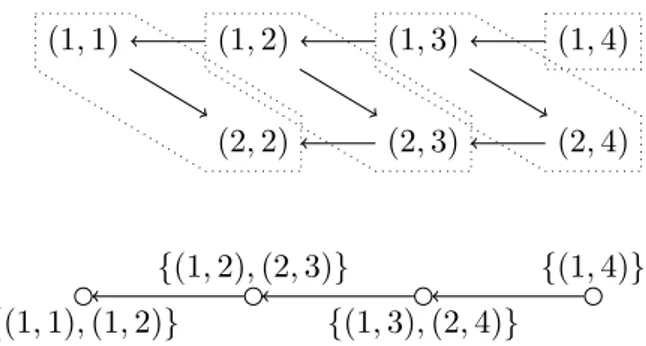
A rotation supernode R0 of a rotation graph R is a subgraph of R with no directed path that both starts and ends in R0 and contains a vertex not in R0. Given a partitioning of the vertices of a rotation graph R into disjoint rotation supernodes, the graph that is induced by contracting each supernode is a directed acyclic graph referred to as a rotation supergraph. A rotation supergraph generalizes the concept of a rotation graph to coarser units of com-putation. Each rotation supernode can be explicitly accumulated to form a transformation and then the rotation supergraph can be applied using matrix–matrix multiplications based on these transformations. Figure 2 illustrates one of many possible ways to form a rotation supergraph (bottom) from a given rotation graph (top).
(1, 1) (1, 2) (1, 3) (1, 4) (2, 2) (2, 3) (2, 4) {(1, 1), (1, 2)} {(1, 2), (2, 3)} {(1, 3), (2, 4)} {(1, 4)}
Figure 2: Illustration of a partitioning of a rotation graph into rotation supernodes (top) and the resulting rotation supergraph (bottom).
2.2 Parallel computing
The parallel computer consists of P = PrPc processors/cores, each running a process with its
own private memory. The processes are arranged in a logical two-dimensional mesh of size Pr× Pc and are labeled with (p, q) where p ∈ {0, 1, . . . , Pr− 1} is the mesh row index and
q ∈ {0, 1, . . . , Pc− 1} is the mesh column index.
The processes communicate by sending explicit messages. Point-to-point messages have non-blocking send semantics and blocking receive semantics, while all collective operations are blocking. These are the semantics used in the Basic Linear Algebra Communication Subprograms (BLACS) library [7], which we used in the implementation. The same semantics can also be obtained using the Message Passing Interface (MPI).
A matrix A is said to be distributed over the process mesh with a two-dimensional block-cyclic distribution with block size nb if the matrix element aij is assigned to process (p, q), where p = b(i − 1)/nbc mod Pr and q = b(j − 1)/nbc mod Pc.
3
The sequential KKQQ HT reduction algorithm
This section recalls the KKQQ HT reduction algorithm [12] since it is the foundation of our parallel formulation. Refer to the original publication for details.
The idea of Moler and Stewart’s algorithm [14] is to systematically reduce the columns of A from left to right using a sequence of rotations applied from the bottom up for each column. After reducing a column, the resulting sequence of rotations is applied to the upper triangular matrix B, which creates fill in the first sub-diagonal and thus changes the structure of B from upper triangular to upper Hessenberg. The next step is to remove the fill in B by a sequence of rotations applied from the right. This step can be viewed as an RQ factorization of a Hessenberg matrix. The resulting rotations are then applied also to A. After applying this procedure to the first n − 2 columns of A, the HT reduction is complete. The orthogonal matrices Q and Z that encode the transformation from (A, B) to (H, T ) can be obtained by accumulating the rotations applied from the left into Q and the rotations applied from the right into Z. The main idea of the KKQQ algorithm is to delay a large fraction of the work involved in the application of rotations in Moler and Stewart’s algorithm until the work can be applied more efficiently (in terms of communication through the memory hierarchy) using matrix–matrix multiplications.
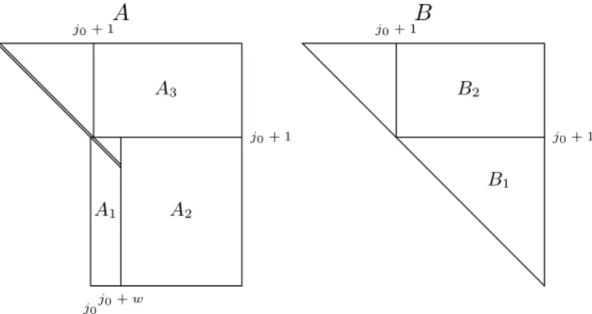
A A1 A2 A3 j0 j0+ w j0+ 1 j0+ 1 B B1 B2 j0+ 1 j0+ 1
Figure 3: Block partitioning of the matrices A and B used by Algorithm 1.
The outer loop on line 1 loops over column panels of A of width w from left to right and j0 denotes the first column index of the current panel. The first row index of the panel is
j0+ 1. The panel is denoted by A1 in Figure 3. The current panel width is determined on
line 2. The matrices A and B are logically partitioned as in Figure 3. Two rotation graphs Rleft (for rotations applied from the left) and Rright (for rotations applied from the right) are initialized on line 4. The rotation graphs are empty in the sense that there are no rotations yet associated with the vertices. The remainder of the outer loop body consists of three phases: the rotation construction phase, where rotations are constructed with a minimum of work performed, the rotation accumulation phase, where the rotations are partitioned into rotation supernodes and explicitly accumulated, and the delayed update phase, where the remaining work is performed by applying the transformations. The three phases are described in more detail below.
Rotation construction: The rotation construction phase encompasses the entire inner loop on line 5. This loop iterates over the columns in the current panel from left to right and j denotes the current column index. The current column is brought up-to-date with respect to delayed updates from previous iterations in the inner loop on line 6. The current column is then reduced on line 7, which generates sequence j − j0+ 1 of Rleft. This newly constructed sequence is then applied to B1from the left on line 8, which creates fill in its first
sub-diagonal. The block B1 is then reduced back to upper triangular form on line 9, which
generates sequence j − j0+ 1 of Rright. This newly constructed sequence is then applied to A1 and A2 from the right on line 10.
Rotation accumulation: The rotation construction phase has generated the two rotation graphs Rleft and Rright. The purpose of the rotation accumulation phase is to partition these graphs into rotation supernodes of an appropriate size and then explicitly accumulate each supernode into a transformation. The supernodes should in general span all ˆw sequences (effectively resulting in a rotation supergraph that is linear) and their size should be such that the transformations are of size close to 2 ˆw × 2 ˆw to minimize the overhead of the accu-mulation [13]. All of this occurs on line 11.
Algorithm 1: The KKQQ [12, Algorithm 3.2] HT reduction algorithm
Data: Matrices A, B ∈ Rn×n, where B is upper triangular, orthogonal matrices Q, Z ∈ Rn×n, and a
block size w ∈ {1, 2, . . . , n}.
// Loop over panels of width w from left to right
1 for j0← 1 : w : n − 2 do
// Determine the current block size
2 w ← min{w, n − jˆ 0− 1};
// THE ROTATION CONSTRUCTION PHASE
3 Partition A and B as in Figure 3;
4 Let Rleft and Rright be empty rotation graphs (no rotations yet attached to the vertices) with ˆw sequences, lower bounds `i= j0+ i, and upper bounds ui= n − 1 for i = 1, 2, . . . , ˆw;
// Loop over the columns in the panel from left to right
5 for j ← j0 : 1 : j0+ ˆw − 1 do
6 Apply sequences 1, 2, . . . , j − j0 of Rleftto the j’th column of A;
7 Reduce the j’th column of A and add the rotations as sequence j − j0+ 1 of Rleft;
8 Apply sequence j − j0+ 1 of Rleftto B1 from the left;
9 Reduce B1 from the right and add the rotations as sequence j − j0+ 1 of Rright;
10 Apply sequence j − j0+ 1 of Rrightto A1 and A2from the right; // THE ROTATION ACCUMULATION PHASE
11 Partition Rleftand Rright into rotation supergraphs and accumulate each rotation supernode into a transformation;
// THE DELAYED UPDATE PHASE
12 Apply the transformations in Rleftto A2 from the left;
13 Apply the transformations in Rleftto QTfrom the left;
14 Apply the transformations in Rrightto A3 from the right;
15 Apply the transformations in Rrightto B2 from the right;
16 Apply the transformations in Rrightto Z from the right;
Delayed updates: The transformations are applied using matrix–matrix multiplications to parts of A, B, Q, and Z in the delayed update phase. The rotations from the left are applied to A2 and QT on lines 12–13. The rotations from the right are applied to A3, B2,
and Z on lines 14–16.
4
Overview of the parallel formulation
Our parallel formulation of Algorithm 1 consists of several parts that are parallelized in different ways. This section gives an overview of the algorithm and identifies the parts and connects them to the underlying sequential algorithm. The details of each part are given separately in Sections 5–8.
The input matrices A, B, QT, and Z are assumed to be identically distributed across the process mesh using a two-dimensional block-cyclic distribution with block size nb. The
notation A(p,q)refers to the submatrix of the distributed matrix A that is assigned to process (p, q). Similarly, the notations A(p,∗) and A(∗,q)refer to the submatrices assigned to mesh row p and mesh column q, respectively.
The rotation graphs Rleft and Rright are represented by two-dimensional arrays of size n × ˆw and are replicated on all processes.
The following are the main parts of the parallel formulation. The update and reduction of the current column of A (lines 6–7) is referred to as UPDATEANDREDUCECOLUMN and is described in Section 5. The application of a sequence of rotations from the left (line 8) is referred to as
ROWUPDATE and is described in Section 6. The reduction of B back to triangular form (line 9) is referred to as RQFACTORIZATION and is described in Section 7. The application of a sequence of rotations from the right (line 10) is referred to as COLUPDATE and is conceptually similar to ROWUPDATE. The accumulation of rotations into transformations (line 11) is referred to as ACCUMULATE and is described in Section 8. The application of a sequence of transformations from the left (lines 12–13) is referred to as BLOCKROWUPDATE and is conceptually similar to ROWUPDATE. Finally, the application of a sequence of transformations from the right (lines 14– 16) is referred to as BLOCKCOLUPDATE and is also conceptually similar to ROWUPDATE.
5
Updating and reducing a single column
The input is a rotation graph and a partial column of a distributed matrix. The purpose is to apply the rotation graph to the column and then reduce it by a new sequence of rotations. Since applying a rotation sequence to only one column is inherently sequential, parallelism can be extracted only by pipelining the application of multiple sequences. Specifically, one process can apply rotations from sequence i while another process applies rotations from sequence i+1. With s sequences, up to s processes can be used in parallel with this pipelining approach. In practice, however, such a parallelization scheme is very fine-grained and leads to a lot of parallel overhead—especially in a distributed memory environment—and therefore requires a sufficiently long column and sufficiently many sequences to yield any speedup. Therefore, we dynamically decide on a subset of the processes (ranging from a single process to the entire mesh) onto which we redistribute the column and apply the sequences in parallel. While this part of the algorithm accounts for a tiny proportion of the overall work, its limited scalability makes it a theoretical bottleneck that ultimately limits the overall scalability of our parallel HT reduction.
6
Wavefront scheduling of a rotation sequence
The dominating computational pattern in Algorithm 1 is the application of a sequence of rotations or transformations and is manifested in ROWUPDATE, COLUPDATE, BLOCKROWUPDATE, and BLOCKCOLUPDATE. There are also close connections to the pattern in RQFACTORIZATION. This section describes a novel scheduling algorithm that is capable of using the processes efficiently and generates a pattern of computation that resembles wavefronts, hence the name. We treat in this section only the special case of applying a sequence of rotations from the left to a dense matrix. The method readily extends to upper triangular matrices, to sequences applied from the right, and to sequences of transformations. We assume that the sequence of rotations is replicated on all processes.
A first observation is that applying rotations from the left does not cause any flow of in-formation across columns of the matrix. Hence, each column can be independently updated. In our parallel setting, this implies that there will be neither communication nor synchro-nization between processes on different mesh columns. Therefore, we may assume without loss of generality that the matrix is distributed on a Pr× 1 mesh, i.e., a mesh with a sin-gle column. For a matrix distributed on a general mesh, one simply applies the scheduling algorithm independently on each mesh column.
The rest of this section is organized as follows. Section 6.1 motivates the need for a more versatile scheduling algorithm by illustrating why a straightforward approach leads to poor
scalability. Section 6.2 gives a high-level overview of the algorithm. Fundamental building blocks of the algorithm are detailed in Section 6.3, and the final details of the algorithm as a whole are given in Section 6.4.
6.1 Why a straightforward approach scales poorly
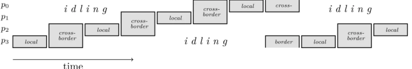
The straightforward approach of applying each rotation completely one after the other does not scale because most of the time only one of the P processes are active and occasionally two processes are active. This is illustrated by the Gantt-chart in Figure 4. Each rotation in the sequence is classified as local if the two affected rows belong to the same process and as cross-border if the two rows belong to different processes. Hence, roughly a fraction (nb− 1)/nb of all rotations are local and only a fraction 1/nb are cross-border.
local cross-border local cross-border local cross-border local cross-border local cross-border local i d l i n g i d l i n g i d l i n g p0 p1 p2 p3 time
Figure 4: Gantt-chart for the straightforward application of a sequence of rotations from the left using a 4 × 1 mesh. At most two processes are active at the same time.
6.2 Overview of the wavefront scheduling algorithm
To improve on the straightforward application it becomes necessary to split the application of a rotation into several independent operations and introduce parallelism through pipelining. Specifically, the columns are partitioned into ˆNb blocks of size ˆnb. The block size ˆnb is
independent of the distribution block size nb, but is closely related to the degree of concurrency
and should be chosen such that ˆNb ≥ Pr in order to use all processes. With fewer than Pr
blocks, there is not enough concurrency to keep all processes busy at the same time.
The ˆNb distributed column blocks are referred to as fragments and play a key role in the
scheduling algorithm. The operations necessary to update a fragment are decomposed into an alternating sequence of local and cross-border actions. A local action is the application of a maximal contiguous subsequence of local rotations, and a cross-border action is the application of a cross-border rotation. Due to the flow of data upwards in each column, the actions associated with a particular fragment need to be performed in a strictly sequential order.
Consider a single fragment at any given moment during the computation. Either the fragment has already been completely updated or there is a uniquely identified next action to perform on that fragment. If the next action is a local action, then the fragment is associated with the process that owns the distribution block affected by the local rotations. If the action is instead a cross-border action, then the fragment is associated with a pair of adjacent processes, namely those that own the two distribution blocks affected by the cross-border rotation. In essence, each fragment is at any point in time associated either with a particular process or with a particular pair of adjacent processes. This association is used to make the scheduling algorithm more efficient.
0 1
2
3 4
5
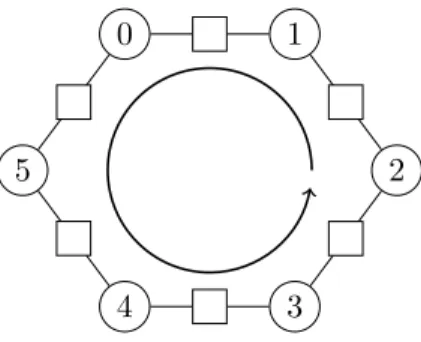
Figure 5: The twelve slots (local slots as circles and cross-border slots as squares) for the case of P = 6 processes. The circular arrow shows how the slots are ordered.
Associated with each process and with each pair of adjacent processes is a slot. A slot contains all the fragments that are currently associated with its related process(es). There are Pr local slots, each associated with a single process, and also P cross-border slots, each
associated with a pair of adjacent processes. As an example, consider the twelve slots for the case Pr= 6 illustrated in Figure 5. The local slots (and also the processes) are identified by circles. The cross-border slots are identified by squares. The adjacency of slots and processes is illustrated by lines. A fragment systematically moves from slot to slot in response to the completion of its actions. The direction in which a fragment moves is indicated by an arrow in Figure 5.
The wavefront scheduling algorithm revolves around the concept of a parallel step. A parallel step is a set of actions of the same type (local or cross-border) for which no two actions belong to fragments residing in the same slot. A parallel step is maximal if it involves one action from every slot of the chosen type. Since the type of action in a parallel step is homogeneous, one can refer to the steps as either local or cross-border. The actions in a parallel step can be performed in a perfectly parallel fashion (see Section 6.3 below) and a maximal step leads to no idling, which makes parallel steps useful as building blocks for an efficient schedule. The aim of the wavefront scheduling algorithm is to construct and execute a shortest possible sequence of parallel steps.
How to obtain a minimal sequence of parallel steps is an open problem. We conjecture that using a greedy algorithm that adheres to the following rules will yield a close-to-optimal solution.
1. Choose between a local and cross-border parallel step based on which type of step will lead to the execution of the most actions.
2. Choose from each slot of the appropriate type (local or cross-border) the fragment that has the most remaining actions.
The rationale behind Rule 1 is to greedily do as much work as possible. The rationale behind Rule 2 is to avoid ending up with a few fragments with many remaining actions and is based on the critical path scheduling heuristic.
6.3 Executing a parallel step
6.3.1 Executing a local parallel step
A local parallel step is perfectly parallel since it involves only local actions and hence requires neither communication nor synchronization. Ideally, the parallel step is maximal and then every process has exactly one task to perform and the tasks have roughly the same execution time as a consequence of the homogeneous block size ˆnb.
6.3.2 Executing a cross-border parallel step
A cross-border parallel step involves pairwise exchanges of data between pairs of adjacent processes. Ideally, the parallel step is maximal and in this case every process would be involved in two unrelated cross-border actions.
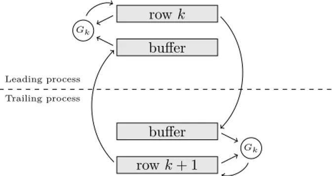
row k buffer Leading process Trailing process buffer row k + 1 Gk Gk
Figure 6: Illustration of a cross-border rotation Gkapplied to rows k and k + 1 of a fragment. The two processes begin by exchanging rows and finish by updating their respective local rows. Figure 6 illustrates how the work of applying a cross-border rotation to a fragment is coordinated between the two processes involved in the operation. A cross-border rotation Gk is applied to rows k and k + 1. The former is held by the so-called leading process and the latter by the so-called trailing process. Both processes begin by sending their respective local rows to the other process. Now each process has a copy of both rows and finishes by updating its local row.
Algorithm 2: Execution of a cross-border parallel step
1 Let p ∈ {0, 1, . . . , P − 1} be the rank of this process;
2 Let L denote the action (if any) in which this process is the leading process; 3 Let T denote the action (if any) in which this process is the trailing process; 4 Let kLand kTdenote the indices of the corresponding cross-border rotations;
5 if L is defined then
6 Send row kL of the fragment associated with L to process (p + 1) mod P ;
7 if T is defined then
8 Send row kT+ 1 of the fragment associated with T to process (p − 1) mod P ;
9 Receive a row from process (p − 1) mod P into a buffer;
10 Update row kT+ 1 of the fragment associated with T using rotation GkT;
11 if L is defined then
12 Receive a row from process (p + 1) mod P into a buffer;
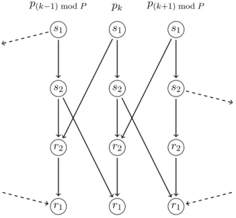
Since a process can be involved in two unrelated cross-border actions in one parallel step, one needs to schedule the sends and receives in a way that avoids deadlock. Algorithm 2 describes one solution to this problem for a general (i.e., not necessarily maximal) cross-border parallel step. A basic observation that is fundamental to the communication algorithm is that if a process is involved in two actions, then it will be the leading process in one of them and the trailing process in the other. That Algorithm 2 is deadlock-free is shown in Proposition 1.
Proposition 1. Algorithm 2 is deadlock-free for any number of processes.
Proof. We first show that deadlock cannot occur for a maximal parallel step. Then we argue that deadlock cannot occur for non-maximal parallel steps either.
Consider a maximal parallel step. Label the two sends by s1and s2 in the order that they are executed by Algorithm 2. Similarly, label the two receives r1 and r2 in the order they are
executed. Since the step is maximal, both L and T will be defined and hence all then-clauses will be executed. Only the ordering of the sends and receives are relevant for the purpose of analyzing for deadlock. Consider any process pk ∈ {0, 1, . . . , P − 1}. Figure 7 illustrates the sequencing due to program order of the two sends and two receives (middle column) executed by process pk. Also shown are the sends and receives of the two adjacent processes (left and right columns, respectively) and the matching of sends and receives. Figure 7 is merely a template from which a complete dependence graph can be constructed for any given P . In the extreme case of P = 2, the left and right columns are actually the same. In the extreme case of P = 1, there is only one column and each send is matched by a receive on the same process. p(k−1) mod P s1 s2 r2 r1 pk s1 s2 r2 r1 p(k+1) mod P s1 s2 r2 r1
Figure 7: Dependencies between sends and receives in Algorithm 2 illustrated for three adja-cent processes.
There can be at most one ready task per column, due to the (vertical) program order dependencies. Furthermore, there is one process dedicated to each column and therefore every ready task will eventually be executed. As a consequence, the only way for deadlock to occur is if the dependence graph contains a directed cycle. Since every edge in Figure 7 is directed
downwards, a directed cycle cannot exist regardless of P . This shows that Algorithm 2 is deadlock-free for maximal parallel steps.
Suppose that the step is not maximal. Then we effectively need to remove some of the nodes and edges in the dependence graph. The arguments used for the maximal case remain valid and hence the algorithm is deadlock-free also for this case.
6.4 The wavefront scheduling algorithm
This section describes the details of the wavefront scheduling algorithm (Algorithm 3).
Algorithm 3: Wavefront scheduling
1 SLis the set of local slots;
2 SBis the set of cross-border slots;
3 loop
// Select non-empty slots of the same type
4 S ← {s ∈ SL∪ SB: Size(s) > 0}; 5 nL← |S ∩ SL|; 6 nB← |S ∩ SB|; 7 if nL> nBthen 8 S ← S ∩ SL; 9 else 10 S ← S ∩ SB;
// Terminate if all actions have been performed
11 if S = ∅ then terminate;
// Extract one fragment from each selected slot
12 F ← {Select(s) : s ∈ S};
// Perform the parallel steps
13 if nL> nBthen
14 Perform a local parallel step on the fragments in F (Section 6.3.1); 15 else
16 Perform a cross-border parallel step on the fragments in F (Section 6.3.2);
// Move (or remove) the updated fragments
17 foreach f ∈ F do
18 if ActionCount(f ) > 0 then
19 Slot(f ) ← Next(Slot(f ));
20 else
21 Undefine Slot(f );
At the top level of Algorithm 3 is a loop that continues until all actions have been per-formed. A subset S of the slots is chosen such that all slots in the set have the same type and contain at least one fragment. The choice is made according to Rule 1 in Section 6.2. The function Size returns for a given slot the number of fragments (possibly zero and at most
ˆ
Nb) that currently resides in that slot. The algorithm terminates when there is no fragment
in any of the slots. The set S of slots is then mapped to a set F of fragments by selecting from each slot the fragment with the most remaining actions. The choice is made according to Rule 2 in Section 6.2. The selection is carried out by the function Select. The parallel step defined by the set of fragments F is performed as described in Section 6.3. Finally, each fragment is either moved to its next slot or removed altogether. The function Slot returns the slot in which a given fragment currently resides (or is undefined if the fragment has been completed). The function Next returns the next slot relative to a given slot. The function
ActionCount returns the number of actions remaining in a given fragment. (a) Before 0 L 1 B 2 L 3 B 4 L 5 B 6 L 7 B number type fragmen ts (b) During 0 L 1 B 2 L 3 B 4 L 5 B 6 L 7 B number type fragmen ts (c) After 0 L 1 B 2 L 3 B 4 L 5 B 6 L 7 B number type fragmen ts
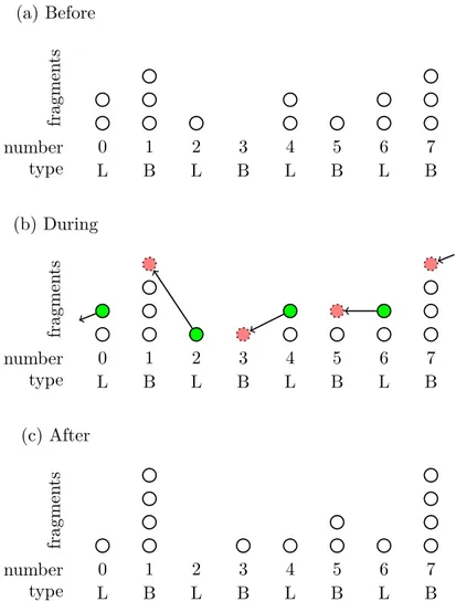
Figure 8: Example illustrating the movement of fragments after an iteration of Algorithm 3 that resulted in the execution of a local parallel step.
Figure 8 provides an example of the movement of fragments after one iteration of Algo-rithm 3 for the case of P = 4 processes. Each fragment is illustrated by a circle and the eight slots are indicated by eight columns labeled 0 through 7 in a clockwise direction relative to Figure 5. Figure 8(a) shows the state of the slots before the iteration. Since there are nL = 4 non-empty local (L) slots but only nB = 3 non-empty cross-border (B) slots, Algorithm 3
will choose to perform a local parallel step and set S = {0, 2, 4, 6}. One fragment from each of the chosen slots will then be selected, and these are shown in green in Figure 8(b). After completing the parallel step, the four selected fragments move to their respective next slots, i.e., from slot s ∈ {0, 1, . . . , 7} to (s − 1) mod 8. The resulting state of the slots after the iteration is shown in Figure 8(c).
The bottom of Figure 9 illustrates a simulated schedule produced by Algorithm 3 for a rotation sequence applied from the right using a 4 × 4 process mesh. The processes are labeled in row-major order, so the first group of four traces belong to the first mesh row and so on. Besides the pipeline startup and shutdown phases, the processes are active all the time. The
Timestep Pro cess c c c c c c u u u u c c c c c c c u c u u u u u c u C u c c C c c C u c c u C c u u u u c u u C u u C u u c c C C u c c C u C c c u C C c u u u u C u u u C u u u C u u u C C C C u C C C u C C C u C C C u u u u C u u u C u u u C u u u C C C C u C C C u C C C u C C C u u u u C u u u C u u u C u u u C C C C u C C C u C C C u C C C u u u u C u u u C u u u C u u u C C C C u C C C u C C C u C C C u u u u C u u u C u u u C u u u C C C C u C C C u C C C u C C C u u u u C u u u C u u u C u u u C C C C u C C C u C C C u C C C u u u u C u u u C u u u C u u u C C C C u C C C u C C C u C C C u u u u C u u u C u u u C u u u C C C C u C C C u C C C u C C C u u u u C u u u C u u u C u u u C C C C u C C C u C C C u C C C u u u u C u u u C u u u C u u u C C C C u C C C u C C C u C C C u u u u C u u u C u u u C u u u C C C C u C C C u C C C u C C C u u u u C u u u C u u u C u u u C C C C u C C C u C C C u C C C u u u u C u u u C u u u C u u u C C C C u C C C u C C C u C C C u u u u C u u u C u u u C u u u C C C C u C C C u C C C u C C C u u u u C u u u C u u u C u u u C C C C u C C C u C C C u C C C u u u u C u u u C u u u C u u u C c C C u C C C u C C C u c C C u u u u C u u u C u u u C u u C c c C u C C C u c C C u c C u u u u C u u u C u u C u C c c c u c C C u c C u c u u u u c u u C u C c u c c u c C u c u u u u u c u u C u C c u c c u c C u c u u u u u c u u C u C c c c u c C u c u u u u c u u C u C c c c u c C u c u u u u c u u C u C c c c u c C u c u u u c u C c c u c u u c c Timestep Pro cess r u u u u c c c c c c c c u u r u u u u u u c c u u c C c c C c u u c C c u u r u u c C c u u c C c c C c u u u c C c u u u u u u c C C c u u c C C c c C C c u u u c C C c r u u u u c C C c u u c C C c c C C c u u u c C c u u u u u u C C c c u u C C c c C C c c u u C c c u u u u C c c u u r C c c C c c u u C c c u u u u u c c C u u C c c C c c C u r u c c C u u u u u u c c C u u u c c C C c c C C u u c c C C u u r u u c C c u u c C c c C c u u u c C c u u u u u u c C C c u u c C C c c C C c u u c C c r u u u u c C c u c C c c C c u u u u u u u u C c c C c c C c c C c c u u r u u u u u u u C c c C c c C c c C c c C u u u u u u r u c c C c c C c c C c c C u u u u u u u u c C c c C c c C c c C c u u r u u c c u u c c c c u c C c u u u c c r u c C c c c u c C c u u u u c c u u C c c C c c u C c c u u c c u c c c c u r c c u u c c u c c c c u c c u r u c c u u c c c c u c C c u u c c u c c c c c c r u u c c u u c c u c c c c r u c c c c u u u u c c c c c c c c r u u u c c c c c c r u u c c c c r u c c Timestep Pro cess u u u u c c c c c c c c u u u u u u u u c C c c C c c C c c C c u u u u u u u u u u u u c C C c c C C c c C C c c C C c u u u u u u u u u u u u u u u u C C C C C C C C C C C C C C C C u u u u u u u u u u u u u u u u C C C C C C C C C C C C C C C C u u u u u u u u u u u u u u u u C C C C C C C C C C C C C C C C u u u u u u u u u u u u u u u u C C C C C C C C C C C C C C C C u u u u u u u u u u u u u u u u C C C C C C C C C C C C C C C C u u u u u u u u u u u u u u u u C C C C C C C C C C C C C C C C u u u u u u u u u u u u u u u u C C C C C C C C C C C C C C C C u u u u u u u u u u u u u u u u C C C C C C C C C C C C C C C C u u u u u u u u u u u u u u u u C C C C C C C C C C C C C C C C u u u u u u u u u u u u u u u u C C C C C C C C C C C C C C C C u u u u u u u u u u u u u u u u C C C C C C C C C C C C C C C C u u u u u u u u u u u u u u u u C C C C C C C C C C C C C C C C u u u u u u u u u u u u u u u u C C C C C C C C C C C C C C C C u u u u u u u u u u u u u u u u C C C C C C C C C C C C C C C C u u u u u u u u u u u u u u u u C C C C C C C C C C C C C C C C u u u u u u u u u u u u u u u u C C C C C C C C C C C C C C C C u u u u u u u u u u u u u u u u c C C c c C C c c C C c c C C c u u u u u u u u u u u u c C c c C c c C c c C c u u u u u u u u c c c c c c c c
Figure 9: Illustration of simulated schedules produced by variants of the wavefront scheduling algorithm on a 4 × 4 process mesh. The label ‘u’ means a local action, ‘r’ a reduction action, ‘c’ (lower case) a single cross-border action, and ‘C’ (upper case) a pair of cross-border actions. Top: Rotations applied from the left to an upper triangular matrix (Section 6). Middle: Rotations created and applied from the right to reduce a Hessenberg matrix to upper triangular form (Section 7). Bottom: Rotations applied from the right to a dense matrix (Section 6).
top of the figure shows a corresponding trace for a rotation sequence applied from the left to an upper triangular matrix. (Note that the time scales in the three subfigures are different.) The mesh columns are less in sync and the load imbalance is more severe than in the dense case. However, the schedule can still activate all processes at the same time.
6.5 Overhead analysis of Algorithm 3
In this section, we analyze the overhead per iteration of the loop in Algorithm 3.
The slot data structures are numbered from 0 to 2P − 1 and accessed in constant time. Each slot contains a set housing the fragments that currently reside in the slot.
Selecting the type of the parallel step and the non-empty slots can be accomplished in Θ(P ) time by visiting each slot. Extracting from each slot a fragment with the most remaining actions can be accomplished in O( ˆNb) time if an unordered set data structure is used and
in O(log ˆNb) time if a priority queue data structure is used. Finally, moving the fragments
can be accomplished in Θ(1) time if an unordered set data structure is used and in O(log ˆNb)
time if a priority queue data structure is used.
In summary, the overhead per iteration is bounded by O(P + ˆNb) if an unordered set data
structure is used and by O(P + log ˆNb) if a priority queue data structure is used. For the
special case ˆNb= P , the overhead is Θ(P ) regardless of the underlying data structure.
Note that the context in this section is a mesh of size P × 1. In reality, the scheduling algorithm is applied independently on each mesh row or mesh column. Thus, for a mesh of size √P ×√P , replace P with√P in all of the above.
7
Wavefront RQ factorization of a Hessenberg matrix
The aim is to reduce an upper Hessenberg matrix to upper triangular form by creating and applying a rotation sequence from the right. The pattern of computation has many similarities with the pattern analyzed in Section 6 but with the addition that the rotations are not known beforehand. This small difference causes profound effects, since it introduces both the need for collective communication and also causes flow of information perpendicular to the flow introduced by the sequence itself. In this section, we show how to extend the algorithm presented in Section 6 to this computational pattern.
The rotation sequence is applied from the right, so the fragments are now row blocks instead of column blocks. Moreover, the fragments are now aligned with the distribution blocks, i.e., a fragment is the same as a distribution row block.
To generate new rotations and replicate them, we need to introduce a few more actions besides the local and cross-border actions. The last local action on a fragment updates a block on the diagonal. We replace this action with a new reduction action and remove the following (and final) cross-border action (if any). The purpose of a reduction action is to reduce the diagonal block and the column immediately to the left. After reducing the diagonal block, the new rotations need to be replicated using a new reduction-broadcast action.
Since the rotations are not known beforehand, the fragments can no longer make progress independently. To account for this, we distinguish between active and inactive fragments. The active fragments are those that can perform their next action and the inactive fragments are the remaining ones, i.e., those whose next action depends on rotations not yet locally available. Each slot now contains a mix of active and inactive fragments. The function ActiveSize returns the number of active fragments in a given slot.
Algorithm 4: Wavefront scheduling for the RQ factorization of a Hessenberg matrix
1 SLi is the set of local slots on process mesh row i ∈ {0, 1, . . . , Pr− 1};
2 SBi is the set of cross-border slots on process mesh row i ∈ {0, 1, . . . , Pr− 1};
3 Let (p, q) be the mesh row and column indices, respectively, of this process; 4 loop
// Select active slots
5 foreach i ∈ {0, 1, . . . , Pr− 1} do 6 Si← {s ∈ SLi ∪ SBi : ActiveSize(s) > 0}; 7 niL← |Si∩ SLi|; 8 niB← |Si∩ SBi|; 9 if niL> niBthen 10 Si← Si∩ SLi; 11 else 12 Si← Si∩ SBi;
// Terminate if all actions have been performed
13 if ∀i ∈ {0, 1, . . . , Pr− 1} : Si= ∅ then terminate;
// Extract one active fragment from each selected slot
14 foreach i ∈ {0, 1, . . . , Pr− 1} do
15 Fi← {ActiveSelect(s) : s ∈ Si}; 16 F ← F0∪ F1∪ · · · ∪ FPr−1;
// Find an active fragment (if any) whose next action is a reduction
17 R ← {f ∈ F : Reduction(f )};
// Perform the parallel steps
18 if npL> npBthen
19 Perform a local parallel step on the fragments in Fp(Section 6.3.1); 20 else
21 Perform a cross-border parallel step on the fragments in Fp(Section 6.3.2);
22 if R 6= ∅ then
23 R = {r};
24 Perform a reduction-broadcast action on the fragment r;
// Move (or remove) the updated fragments
25 foreach f ∈ F do
26 if ActionCount(f ) > 0 then
27 Slot(f ) ← Next(Slot(f ));
28 else
The details of the extended wavefront scheduling algorithm are presented in Algorithm 4. The new predicate Reduction, line 17, returns true if the next action on a given fragment is a reduction action. Unlike the original algorithm, the extended algorithm needs to keep track of the progress of all processes and not only the processes in its own mesh row. The need for this extra bookkeeping is to be able to determine when a process should execute the reduction-broadcast actions, see line 22–24. The function ActiveSelect, which replaces Select, returns one of the active fragments from a given slot.
The middle of Figure 9 illustrates a schedule produced by Algorithm 4 using a 4 × 4 mesh. The reduction-broadcast action introduces a synchronization point that leads to significant overhead throughout the execution. The amount of idling would be less if the number of fragments was larger relative to the number of processes.
7.1 Overhead analysis of Algorithm 4
In this section, we analyze the overhead per iteration of the loop in Algorithm 4.
The following assumes that the mesh size is √P ×√P . The number of fragments is denoted by Nband is independent of P as Nb depends only on the size of the problem size n and the distribution block size nb.
Selecting active slots can be accomplished in Θ(P ) time by scanning through all of the√P slots associated with each of the√P mesh rows. Extracting from each selected slot a fragment with the most remaining actions can be accomplished in O(√P Nb) time if an unordered set
data structure is used and in O(√P log Nb) time if a priority queue data structure is used.
Finally, moving the fragments can be accomplished in Θ(√P ) time if an unordered set data structure is used and in O(√P log Nb) time if a priority queue data structure is used.
In summary, the overhead per iteration is bounded by O(P +√P Nb) if an unordered set
data structure is used and by O(P +√P log Nb) if a priority queue data structure is used.
8
Accumulation of rotations into transformation matrices
The rotations from both sides are accumulated into transformations. The transformations should align (whenever possible) such that they act on two full and adjacent distribution block rows/columns. This implies that the typical size of a transformation matrix is 2nb× 2nb.
Parallelism in the accumulation is exploited by assigning to each process a subset of the accumulation tasks. After the local accumulation phase, the resulting transformations are replicated across the relevant subsets of the mesh.
9
Computational experiments and results
To analyze the performance, scalability, and bottlenecks of our proposed parallel HT reduction algorithm, we performed a number of computational experiments. Details of the implemen-tation are given in Section 9.1. The setups of the experiments and the parallel computer systems are described in Section 9.2. The results of the experiments are summarized briefly in Section 9.3 followed by details of each experiment in the subsequent Sections 9.4–9.6.
9.1 Implementation details
The algorithm is implemented in Fortran 90/95 and uses the BLAS library for basic matrix computations, the BLACS library for inter-process communication, and auxiliary routines from the ScaLAPACK library.
The block sizes ˆnbused by the wavefront scheduling algorithm were set on a per-call basis
to the largest (although never smaller than 8) that exposes sufficient parallelism to activate all processes. For the row update of B, the block size was set to half the typical value in order to compensate for the load imbalance caused by the upper triangular structure.
The input matrices Q and Z are treated as dense without structure.
9.2 Experiment setup
Two different parallel computer systems were used in the experiments: Triolith at the National Supercomputer Centre (NSC) at Linköping University and Abisko at the High Performance Computing Center North (HPC2N), at Umeå University. See Table 1 for details.
Table 1: Information about the Abisko and Triolith systems.
Abisko 64-bit AMD Opteron Linux Cluster
Processors Four AMD Opteron 6238 processors (12 cores) per node Interconnect Mellanox Infiniband
Compiler Intel compiler
Libraries Intel MPI, ACML 5.3.1 (includes LAPACK functionality), ScaLAPACK 2.0.2
Triolith 64-bit HP Cluster Platform 3000 with SL230s Gen8 compute nodes
Processors Two Intel Xeon E5-2660 processors (8 cores) per node Interconnect Mellanox Infiniband
Compiler Intel compiler
Libraries Intel MPI, Intel MKL 11.3 (includes ScaLAPACK and LAPACK functionality)
Each test case is specified by four integer parameters: the problem size n, the distribution block size nb, and the process mesh size Pr× Pc. Except n, all parameters are tunable and
can be chosen to maximize performance. Since exhaustive search for optimal parameters is prohibitively expensive, preliminary experiments were used to determine a reasonable block size nb. Only square meshes (Pr = Pc) were considered.
The input matrices are randomly generated with elements drawn from the standard normal distribution. The time required by the initial reduction of B to triangular form is not included in the measurements.
9.3 Summary of the experiments
Three sets of experiments were performed:
• Experiment 1: Reasonable distribution block sizes
The purpose of this experiment was to determine a reasonable distribution block size to use for the subsequent experiments. The results of the experiment indicate that nb = 100 is reasonable on both machines. See Section 9.4 for details.
• Experiment 2: Scalability
The purpose of this experiment was to evaluate the weak and strong scalability relative to a state-of-the-art sequential implementation [12]. See Section 9.5 for details.
• Experiment 3: Bottlenecks
The purpose of this experiment was to characterize the cost and scalability of the major parts of the parallel algorithm and identify bottlenecks that currently limit its scalability. See Section 9.6 for details.
9.4 Experiment 1: Reasonable distribution block sizes
The distribution block sizes nb ∈ {40, 60, 80, . . . , 160} were tested on a problem of size n =
4000 and mesh of size Pr = Pc= 4 with the aim of finding a reasonable block size to use for the subsequent experiments. The parallel execution times (in seconds) on both machines are shown in Table 2. These results indicate that nb= 100 is reasonable on both machines.
Table 2: Impact of nb on Triolith and Abisko (n = 4000, Pr= Pc= 4). Times in seconds.
nb= 40 nb= 60 nb= 80 nb= 100 nb= 120 nb= 160
Triolith 32 28 28 27 27 28
Abisko 66 57 54 53 53 56
9.5 Experiment 2: Scalability
The strong scalability of the parallel algorithm was measured in terms of speedup rela-tive to a state-of-the-art sequential implementation of KKQQ [12] for problems of size n ∈ {4000, 8000, 12000, 16000} and meshes of size Pr× Pc for Pr= Pc∈ {1, 2, . . . , 10}.
0 10 20 30 40 50 60 70 80 90 100 0 2 4 6 8 10 12 14 16 18 Number of processes Speedup Triolith n=16000 n=12000 n=8000 n=4000 0 10 20 30 40 50 60 70 80 90 100 0 2 4 6 8 10 12 14 Number of processes Speedup Abisko n=16000 n=12000 n=8000 n=4000
Figure 10: Strong scalability (speedup relative to KKQQ on one core).
The results of the strong scalability experiments are shown in Figure 10. The sequential algorithm is faster on one core than the parallel algorithm. The strong scalability increases with larger problem sizes. The parallel efficiency is low, which indicates that much larger problems than those tested are necessary for the algorithm to run efficiently.
Both memory-constrained and time-constrained forms of weak scalability were analyzed. The memory-constrained weak scalability was measured by scaling up the problem size n with the number of processes to keep the memory required per process constant. Specifically,
0 100 200 300 400 500 600 700 800 900 1000 0 2 4 6 8 10 12 14 16 18 1000 1000 4000 2520 8000 4000 12000 5241 16000 6350 20000 7368 24000 8320 28000 9221 31000 9868 Number of processes Speedup Triolith Memory constrained Time constrained 0 100 200 300 400 500 600 700 800 900 1000 0 2 4 6 8 10 12 14 16 1000 1000 4000 2520 8000 4000 12000 5241 16000 6350 20000 7368 24000 8320 28000 9221 31000 9868 Number of processes Speedup Abisko Memory constrained Time constrained
Figure 11: Weak scalability (speedup relative to KKQQ on one process). The labels show the scaled problem size n.
for a problem of size n1 on one process, the problem size on P processes was set to n1√P . The time-constrained weak scalability, on the other hand, was measured by scaling up the problem size with the number of processes to keep the flops required per process constant. Specifically, for a problem of size n1 on one process, the problem size on P processes was set to n1√3p.
The results of the weak scalability experiments, with n1 = 1000, are shown in Figure 11.
The memory-constrained problem scales well using up to 256 processes on both machines. Adding more cores is not beneficial, due to that the time for communication and synchroniza-tion will increase more and more, relative to the time for computasynchroniza-tion. The time-constrained setup scales well using up to 64 processes, adding more processes is not fruitful at all. The setup suffers from a small n1 resulting in smaller and smaller local problem size when the mesh size, and therefore the amount of communication, is increased. A larger n1 allows the
use of more cores efficiently. Using n1= 2000 allows for using up to 256 processes on Abisko,
instead of 64, before the peak is reached.
9.6 Experiment 3: Bottlenecks
Profiling data was gathered in an effort to identify bottlenecks that can explain the limited scalability observed in Section 9.5. For each call to a major subroutine, measurements of the parallel execution time, the flop count, and the time spent in numerical computation were made. For the purpose of these measurements, barrier synchronizations were inserted before each subroutine call. In this way, load imbalances caused by one subroutine call do not affect the measurements of the next. The names of the subroutines referred to in this section correspond to the definitions in the end of Section 4.
The parallel cost of a parallel algorithm that takes T seconds to execute on P processes is defined as the product P T . The parallel cost of a subroutine is the parallel cost that is attributable to that subroutine. The relative costs of each subroutine for n = 8000 on various meshes are shown in Figure 12. The results are qualitatively similar on both machines. Two bottlenecks can be identified from these results. First, the UPDATEANDREDUCECOLUMN subroutine, whose cost is almost negligible on one core, accounts for more than 30% of the
Figure 12: Cost distribution across subroutines for n = 8000 on various process meshes. The pattern orderings in the bar plots are the same as in the legend.
cost on 100 processes. This can be understood since this part of the computation is barely parallelizable, as explained in Section 5. Second, the RQFACTORIZATION subroutine accounts for almost 40% of the cost on 100 processes whereas it accounts for around 20% on one core. This can be understood in part by the larger overhead of the extended wavefront scheduling algorithm (relative to the standard wavefront scheduling algorithm; see Section 7.1) and in part by the additional synchronization and communication overheads inherent in the computation (see Section 7).
0 10 20 30 40 50 60 70 80 90 100 0 10 20 30 40 50 60 70 Number of processes Speedup
Triolith unblocked routines
COLUPDATE( A ) RQFACTORIZATION( B ) ROWUPDATE( B ) UPDATEANDREDUCECOL 0 10 20 30 40 50 60 70 80 90 100 0 10 20 30 40 50 60 70 80 90 100 Number of processes Speedup
Triolith blocked routines
BLOCKCOLUPDATE( AB ) BLOCKCOLUPDATE( Z ) ACCUMULATE( COLS ) BLOCKROWUPDATE( Q ) BLOCKROWUPDATE( A ) ACCUMULATE( ROWS )
Figure 13: Speedup for each subroutine on Triolith for n = 8000.
0 10 20 30 40 50 60 70 80 90 100 0 5 10 15 20 25 30 35 Number of processes Speedup
Abisko unblocked rountines
COLUPDATE( A ) RQFACTORIZATION( B ) ROWUPDATE( B ) UPDATEANDREDUCECOL 0 10 20 30 40 50 60 70 80 90 100 0 5 10 15 20 25 30 35 40 45 Number of processes Speedup
Abisko blocked routines
BLOCKCOLUPDATE( AB ) BLOCKCOLUPDATE( Z ) ACCUMULATE( COLS ) BLOCKROWUPDATE( Q ) BLOCKROWUPDATE( A ) ACCUMULATE( ROWS )
Figure 14: Speedup for each subroutine on Abisko for n = 8000.
An alternative view of the profiling data is depicted in Figures 13 and 14. These figures show the relative speedups of the subroutines defined as the ratio of the wall clock time at-tributable to a subroutine when running on one core to the wall clock time when running the subroutine on multiple cores. The wall clock times used in these calculations were obtained by dividing the parallel cost of the subroutine with the number of processes. The coarse-grained and highly parallel blocked routines scale essentially linearly on both machines1. The
unblocked subroutines have poorer scalability, which is especially true for RQFACTORIZATION and UPDATEANDREDUCECOLUMN. The tool Allinea Map2 reveals that our algorithm uses 41% for communication using 16 processes, and the fraction increases to 58% using 36 processes. Looking at the unblocked routines RQFACTORIZATION and UPDATEANDREDUCECOLUMN, the com-munication fraction increases from 44% to 76% and from 91% to 94% when when going from 16 to 36 processes. For the blocked routine BLOCKROWUPDATE(A), the communication fraction decreases from 38% to 32% when increasing the number of processes from 16 to 36. Thus, the heavy communication in the unblocked routines overshadows the nice scaling properties of the blocked routines.
9.7 The parallel two-stage approach
The sequential two-stage approach can in some cases compete with the sequential (one-stage) KKQQ algorithm [12]. However, the parallel two-stage algorithm proposed in [1] do not include the cost-reducing innovations discovered later by [12]. In addition, the complexity of the two-stage approach and the extra arithmetic operations leads to poor performance and scalability. Specifically, running the parallel two-stage algorithm [1] on the weak scaling experiment as in Section 9.5 requires a problem of size n = 5000 and a 5 × 5 mesh before any speedup over sequential KKQQ can be observed. The first stage takes less time than the second, despite the workload ratio being in favor of the second stage. The scheduling ideas presented in this paper can potentially be adapted to the two-stage approach.
10
Conclusion
We proposed a novel wavefront scheduling algorithm capable of scheduling sequences of ro-tations or general transformations on matrices distributed with a two-dimensional block-cyclic distribution. We applied the scheduling algorithm to several parts of a distributed triangular reduction algorithm and obtained a new formulation of Hessenberg-triangular reduction for distributed memory machines. Experiments show that the parallel implementation of the distributed HT-reduction algorithm is scalable, but its behavior is lim-ited by poor scalability of two of the major subroutines. To significantly improve the results, both of these bottlenecks need to be addressed.
The difference of using Householder reflections in the Hessenberg reduction and sequences of Givens rotations in the Hessenberg-triangular reduction has far-reaching consequences. Applying a Householder reflection onto an n × n matrix involves Θ(n2) operations and can use up to p = n2processors. The communication necessary would be one reduction per row or column of the matrix. With the maximum number of processors and a tree-based reduction, the communication cost would be (ts+ tw) log2p, where ts is the latency and tw the inverse bandwidth. On the other hand, applying a sequence of Givens rotations onto an n × n matrix also involves Θ(n2) operations but can use only up to p = n processors. The amount of communication overhead depends on the chosen data distribution and rotation sequences are applied from both sides in the Hessenberg-triangular reduction, which implies that the distribution needs to strike a balance between the costs of the two cases, i.e. updates from
on 100 cores, there are only 50 FPUs available. This is a potential explanation for why the speedup on Abisko is less than 50 on 100 cores.
2
left and right. The communication overhead per row or column of the matrix is proportional to the number of distribution block boundaries that need to be traversed. All of this is on top of the added complexity of the wavefront scheduling algorithm that is necessary to keep all processors busy. All said and done, these factors explain some of the difficulties in obtaining a scalable Hessenberg-triangular reduction implementation.
Acknowledgments
We thank the High Performance Computing Center North (HPC2N) at Umeå and National Supercomputer Centre (NSC) at Linköping for providing computational resources and valu-able support during test and performance runs. This project was funded from the European Unions Horizon 2020 research and innovation programme under the NLAFET grant agree-ment No 671633.
References
[1] B. Adlerborn, K. Dackland, and B. Kågström. Parallel Two-Stage Reduction of a Regular Matrix Pair to Hessenberg-Triangular Form. In In T. Sorevik, F. Manne, R. Moe, and A. H. Gebremedhin, editors, volume 1947 of Lecture Notes in Computer Science, PARA ’00, pages 92–102. Springer-Verlag, 2000.
[2] B. Adlerborn, K. Dackland, and B. Kågström. Parallel and blocked algorithms for re-duction of a regular matrix pair to hessenberg-triangular and generalized schur forms. In Proceedings of the 6th International Conference on Applied Parallel Computing Advanced Scientific Computing, PARA ’02, pages 319–328. Springer-Verlag, 2002.
[3] B. Adlerborn, B. Kågström, and D. Kressner. A parallel qz algorithm for distributed memory hpc systems. SIAM J. Sci. Comput., 36(5):C480–C503, 2014.
[4] Björn Adlerborn, Bo Kågström, and Daniel Kressner. Applied Parallel Computing. State of the Art in Scientific Computing: 8th International Workshop, PARA 2006, Umeå, Sweden,Revised Selected Papers, chapter Parallel Variants of the Multishift QZ Algo-rithm with Advanced Deflation Techniques, pages 117–126. LNCS 4699. Springer Berlin Heidelberg, Berlin, Heidelberg, 2007.
[5] C Bischof. A summary of block schemes for reducing a general matrix to Hessenberg form. Technical report ANL/MSC-TM-175, Argonne National Laboratory, 1993. [6] C. H. Bischof and C. F. Van Loan. The W Y representation for products of Householder
matrices. SIAM J. Sci. Statist. Comput., 8(1):S2–S13, 1987.
[7] L. S. Blackford, J. Choi, A. Cleary, E. D’Azevedo, J. W. Demmel, I. Dhillon, J. J. Dongarra, S. Hammarling, G. Henry, A. Petitet, K. Stanley, D. Walker, and R. C. Whaley. ScaLAPACK Users’ Guide. SIAM, Philadelphia, PA, 1997.
[8] K. Dackland and B. Kågström. Blocked algorithms and software for reduction of a regular matrix pair to generalized Schur form. ACM Trans. Math. Software, 25(4):425–454, 1999.
[9] K. Dackland and B. Kågström. Reduction of a Regular Matrix Pair (A, B) to Block Hessenberg Triangular Form. In In J. Dongarra, K. Madsen, and J. Waśniewski, editors, volume 1041 of Lecture Notes in Computer Science, PARA ’95, pages 125–133, 1995. [10] K. Dackland and B. Kågström. A ScaLAPACK-Style Algorithm for Reducing a Regular
Matrix Pair to Block Hessenberg-Triangular Form. In Applied Parallel Computing Large Scale Scientific and Industrial Problems: 4th International Workshop, PARA’98 Umeå, Sweden, June 14–17, 1998 Proceedings, pages 95–103. Springer Berlin Heidelberg, 1998. [11] B. Kågström and D. Kressner. Multishift variants of the QZ algorithm with aggressive early deflation. SIAM J. Matrix Anal. Appl., 29(1):199–227, 2006. Also appeared as LAPACK working note 173.
[12] B. Kågström, D. Kressner, E.S. Quintana-Orti, and G. Quintana-Orti. Blocked Algo-rithms for the Reduction to Hessenberg-Triangular Form Revisited. BIT Numerical Mathematics, 48(3):563–584, 2008.
[13] B. Lang. Using Level 3 BLAS in Rotation-Based Algorithms. SIAM J. Sci. Comput., 19(2):626–634, 1998.
[14] C.B. Moler and G.W. Stewart. An Algorithm for Generalized Matrix Eigenvalue Prob-lems. SIAM J. Numer. Anal., 10(2):241–256, 1973.
[15] R. C. Ward. The combination shift QZ algorithm. SIAM J. Matrix Anal. Appl, 12(6):835– 853, 1975.