Corruption and Growth - A cross-country study for 2004-2008

Corruption and Growth

A cross-country study for 2004-2008

Bachelor‟s thesis within Economics Author: Julia Ling

Malin Nordahl Tutor: Johan Klaesson

Johan P Larsson Jönköping May 2011

Bachelor‟sThesis in Economics

Title: Corruption and Growth – A cross-country study for 2004-2008

Author: Julia Ling

Malin Nordahl

Tutor: Johan Klaesson

Johan P Larsson

Date: May 2011

Subject terms: Corruption, Corruption Perceptions Index, Development, Economic Growth, GDP growth

Abstract

Economic growth in a country can be explained by numerous variables, both positive and negative. Increasing levels of education, investment and openness are examples of factors generally believed to have positive effects on the economic progress, while corruption is one of the factors often regarded as detrimental to economic growth.

The purpose of this thesis is to measure and analyze if the levels of perceived corruption in a cross-section of countries have affected their economic growth rates over the years 2004-2008. The study is carried out with four regressions on a sample of 123 countries and eight variables for the time period in question. The models are constructed on the basis of both the neoclassical growth theory and the endogenous growth theory.

The found result contradicts the expected outcome; it shows that the perceived levels of corruption are significantly and positively correlated with economic growth.

It is however found that countries with widespread corruption, in general developing countries, have experienced high economic growth over these years. A correlation the authors argue can explain the unexpected sign of the corruption variable.

Kandidatuppsats i Nationalekonomi

Titel: Korruption and tillväxt – En landsomfattande studie för åren 2004-2008

Författare: Julia Ling

Malin Nordahl

Handledare: Johan Klaesson

Johan P Larsson

Datum: Maj 2011

Ämnesord: BNP-tillväxt, Corruption Perceptions Index, ekonomisk tillväxt, korruption, utveckling

Sammanfattning

Ett lands ekonomiska tillväxt kan förklaras av otaliga variabler, både positiva och negativa. Ökade utbildningsnivåer, investeringar och öppenhet är exempel på variabler som anses påverka ekonomisk utveckling positivt, medan korruption är en av dem som anses skada ekonomisk tillväxt.

Syftet med denna uppsats är att mäta och analysera om nivåerna av upplevd korruption i ett tvärsnitt av länder har påverkat deras ekonomiska tillväxttakt mellan åren 2004-2008. Studien är genomförd genom fyra regressioner med en urvalsstorlek på 123 länder och åtta variabler för tidsperioden i fråga. Modellerna är konstruerade utifrån neoklassisk tillväxtteori och endogen tillväxtteori.

Det funna resultatet motsäger det förväntade resultatet: det visar att nivåerna av upplevd korruption är signifikant och positivt korrelerat med ekonomisk tillväxt.

Det är emellertid också funnet att länder med utbredd korruption, generellt utvecklingsländer, har upplevt hög ekonomisk tillväxt under de här åren. En korrelation som författarna menar kan förklara det oväntade tecknet av korruptionsvariabeln.

i

Table of Contents

1

Introduction ... 1

2.

Background on corruption ... 3

3

Theories on Economic Growth ... 6

3.1 Neoclassical Growth Theory ... 6

3.2 Endogenous Growth Theory ... 7

3.3 Related empirical studies ... 9

4

Model ... 11

5

Empirics ... 14

5.1 Results of the estimated coefficients ... 14

5.2 Other tests of the model ... 16

5.3 Discussion ... 17

6

Conclusion ... 22

ii

Figures

Figure 3-1 Solow’s growth model ...6

Figure 5-1 Scatter plot: CPI v. GDP growth per capita ... 15

Figure 5-2 Scatterplot: CPI v. Initial GDP per capita ... 19

Figure 5-3 Annual growth rates 2004-2008 ... 19

Figure 5-4 Scatterplot: Initial GDP per capita v. Capital formation ... 20

Tables

Table 5-1 Descriptive statistics... 14

Table 5-2 Regression output ... 15

Table 5-3 White’s test ... 16

Table 5-4 VIF ... 17

Table 5-5 Normality test ... 17

Appendix 1

Appendix 1B Countries in Latin America and Sub-Sarahan Africa ... 27

Appendix II

Appendix III

1

1

Introduction

During the last centuries the world has experienced an enormous increase in economic welfare. People today have access to goods and services such as computers, cellular phones, health care and insurance; things their great grandparents could not even have dreamed of. The possibilities for a young person today are countless, and the standard of living has never been this high. Yet this is only true for a fraction of the world‟s population. According to the International Monetary Fund (2010) as many as 150 out of the total 193 countries (United Nations, 2006) in the world are classed as developing or emerging economies. In 2005 1.4 billion people lived in extreme poverty, below $1.25/day, (United Nations, 2010), and over three billion people lived on less than $2.50 per day (Global Issues, 2010). Furthermore, these people are hit much harder than the world‟s rich population when downturns strike, and the recent economic crisis is estimated to have caused an additional 64 million people to live in extreme poverty (United Nations, 2010). Countries with historically low levels of GDP per capita tend to be trapped in stagnation (Easterly, 2001). Though some determining factors seem more plausible than others in explaining growth, or its absence, there is no consensus on which ones are the most important. The notion of which variables are important depends on the perspective taken by the observer. From the standpoint of neoclassical theory one would give precedence to factors affecting capital accumulation, labor force growth and productivity growth (Todaro & Smith, 2006). Someone favoring the endogenous point of view on the other hand would argue that any variable accounting for the level of human capital in a country is of prominent significance. Still others argue that development requires good governance; aid and other intentions to increase economic growth, whatever they may consist of, seem to lose its effectiveness in the absence of a sound and stable political environment (Jain, 2001).

One phenomenon that is believed to affect economic growth, but not yet determined in which direction or through what channels, is corruption. Public corruption is commonly defined as the misuse of public office for private gain (Svensson, 2005). This definition would, for instance, include officials selling government property, accepting bribes in public procurement, and misappropriation of government funds. Bribery arises in response to both good and bad policies, to either escape a penalty for violating the good policy or to circumvent the bad (Djankov, LaPorta, Lopez-de-Silanes & Schleifer cited in Svensson, 2005), and can thus prevail in any political environment. According to Rose-Ackerman (1997) the extent of corruption depends on the magnitude of the expected benefits and costs associated with a bribe, and the willingness of firms and individuals to pay a bribe to obtain the benefit or avoid the cost.

Leff (1964: 8) chooses to define corruption as “an extra-legal institution used by individuals or groups to gain influence over the actions of the bureaucracy”. Thus suggesting that corruption in itself is a neutral concept and only implies that these people engage in the decision making process to a larger extent than would be the case in the absence of corruption. Measuring corruption therefore only provides knowledge about the political system in effect, contrasted with the official one. The question of whether the corrupt acts are detrimental or beneficial for economic growth is thus not answered simply by looking at the degree of corruption, but rather by looking at if the groups, companies, and individuals gaining access to the decision making will promote growth more than the government would have.

2

Leff (1964) together with other scholars (e.g. Acemoglou & Verdier, 1998, 2000; Lui, 1985) suggest that corruption has, or might have, a positive impact on growth. The argument being that when the government is indifferent or hostile to efforts promoting growth, corruption would lead to more efficient allocation of resources (Leff, 1964).

The role played by corruption is evidently difficult to observe, and no consensus or general opinion of its effects on growth exists. Its existence can however not be disputed, and the question remains: what effect does it have on economic growth?

The purpose of this thesis is to make an effort to measure and analyze to which extent the level of perceived corruption in a cross-section of countries affects their economic growth rates. The question researched in this thesis is:

Is the perceived level of corruption in a country related to its economic growth rate?

The thesis will be divided as followed. Section 2 will give a general background, discussing the concept of corruption, together with a description of the CPI. In section 3 there will be an outline of the theories of economic growth, followed by the statistical framework in section 4. Section 5 presents the empirical findings and the analysis. The thesis will be concluded in the last section of the thesis.

3

2. Background on corruption

Before making an effort to measure, analyze and discuss the effects of corruption, it is appropriate to define the concept. This section is included with the intention to provide the reader with a deeper knowledge and understanding of corruption as a phenomenon. It explains the cause and consequences of corruption, furthermore it explains the measure of perceived corruption, the Corruption Perception Index (CPI), published annually by Transparency International.

2.1 Corruption

Corruption is a phenomenon present in all cultures and societies. It has always existed, but to different extents and with a variety of consequences (Bardham, 1997). To measure it, a definition is needed A consensus seems virtually impossible however – the varying backgrounds, traditions, and cultures of individuals will inevitably result in an endless variation of definitions. According to Treisman (2000) and Dreher, Kotsogiannis and McCorriston (2007), corruption is caused and characterized by historical and cultural factors, economic development, and political institutions. Old traditions and rituals of bribery and the like are still alive and characterize the corrupt activities in present time. Gift-giving and receiving are referred to as corruption in some countries, but not in others. In its simplest way, it has become standard to define it as “the use of public office for private gain

… a misallocation of resources and inefficiency” (Gyimah-Brempong, 2002: 186). This definition

does thus not include illegal operations such as fraud, money laundering, and black market actions (Jain, 2001).

Philp (2007) puts forward three categories of corruption; grand, legislative, and bureaucratic. Grand corruption is the misuse of power by public officials. Officials make policy decisions based on their own interests instead of serving the public in policy decisions. Legislative corruption affects the voting results since the legislators are bribed by interest groups and other lobbyists. Bureaucratic corruption is the most common form of corruption and involves three parts (Jain, 2001). A public official violates the position to benefit a third part which returns the favor by paying the official off the record. The second act, the public, who is supposed to benefit from the action, is excluded (Philp, 2007).

Corruption is both an economic and political issue. It is most common where other forms of institutional problems exist and where inefficient bureaucracy is present (Jain, 2001). Treisman (2000) argues that developing countries are more likely to have high levels of corruption than developed countries. One explanation suggested is that the boundaries between public and private areas are less pronounced in emerging countries. Moreover, during times of economic progress, corruption is an appealing way for the public official to make personal gain (Treisman, 2000). In order to attain economic progress and growth, policy implications against corruption therefore have to start within the political institutions (Jain, 2001).

This is in line with the view of Shleifer and Vishny (1993) that there are two ways for corruption to hurt economic development, the first one being the structure of the government in the country; a weak government increases the incentive for public officials to take advantage of the system through corruption. The other way is through the secrecy

4

by necessity associated with the corrupt activity. Since some goods and services are easier to collect bribes for secretly, government officials might use their power to increase the level of demand for such products, by decreasing the supply of any substitutable good. The officials thus relocate economic activity in an inefficient way, which in turn decreases the growth.

Furthermore, Mauro (1995) has found that corruption lowers private and public investment in countries. Low investment results in decreasing growth. Richer countries tend to have higher bureaucratic efficiency. Mauro draws the conclusion that there is a strong correlation between bureaucratic efficiency and political stability. A high level of bureaucracy has a propensity to increase growth. On the other side, bureaucratic inefficiency tends to cause low growth.

Another channel through which corruption affects an economy negatively is its harmful effects on innovative activities. Public officials take advantage of the inefficient bureaucracy to gain from innovators and new-established firms, making investments in innovations risky and less profitable.

Corruption can also affect the level of public and government expenditure. Officials tend to allocate their spending to sectors in which they can easily practice corrupt actions (Mauro, 1997). Ades and Di Tella writes that corruption is also found to be affected by the level of openness in an economy; a low corruption level is related to high openness (cited in Mauro, 1997).

Corruption also tends to foster unequal opportunities, leading to higher income inequality and larger gaps between income levels. There is a tendency of multicollinearity in the economy, since corruption, regulations, and governmental systems are difficult to separate empirically (Mo, 2001).

An important remark to make is on the problem of causality, that is, whether corruption affects growth or if economic growth affects the corruption level in a country. Brown and Shackman (2007) find that economic growth affects corruption positively in the short run and negatively in the long run, as opposed to the general opinion. Both views exist and evidence shows that causality is present in both directions. Nevertheless, the overall consensus based on empirics is that corruption negatively affects economic growth either directly or indirectly; through e.g. investment or trade.

Despite this, the implications for policy making are not very straightforward. It is also found that there might be too expensive to eliminate all corruption in a country. There is a trade-off between implementing property rights completely or allow corruption to exist. Therefore, a country could be better off with a low level of corruption than no corruption at all (Acemoglou and Verdier, 1998).

The definition of corruption used throughout this thesis is coming from Transparency International. Transparency International defines corruption as „the abuse of public office for private gain‟ (Transparency International, 2011b).

5

2.2 CPI

Corruption as a concept includes illegal actions, not mentioned in public charters. Due to the fact of many definitions, there is difficult to generalize and measure levels of corruption. The survey may vary depending on what sectors and actors which are involved. It may also depend on the degree of impact corruption has or how it is formalized. Actual corruption levels are difficult to measure (Andersson & Heywood, 2009). Instead, Transparency International (TI) uses a Corruption Perceptions Index (CPI), measuring the perceived levels of corruption. The index has existed since 1995. The index is a composite index and ranks countries based on a combination of foundations. Different surveys, polls, and experts rank countries based on the perceived levels of corruption in the public sector. In order to be included in the list, a country must be present in at least three of the total number of surveys for a given year. As a result, CPI values depend on information availability (Transparency International, 2011c).

Other measures of corruption are given out by the International Country Risk Guide and the World Bank (Svensson, 2005).

Andersson and Heywood (2009) discuss three concerns with the CPI measurement. The first one is that the CPI only measures perceptions and not real levels of corruption. Perceptions can have influence on the population‟s believes of corrupt activities and the incentives to corrupt might rise if the country has high perceived levels of corruption. CPI puts emphasize on the bribe takers and believes bribes are only paid when necessary and not used as a mean to keep good relationships. The second problem is the different measures used by the different institutions. All surveys measure the perceived levels of corruption based on their own belief of what corruption is which can lead to biased results. The third issue is the ranking system TI uses. A country can receive a score from 0,0-10,0; zero indicating high perceived corruption and 10 no corruption. The countries are then ranked based on the score. Small differences in scores may have more than proportional differences in rank.

The CPI has received more critics. CPI surveys have differed from year to year since the start in 1995. It is therefore difficult to receive a non-biased measure when comparing rankings and analyzing trends from different years.

Moreover, those who are involved in corrupt activities abroad and not in the home country are not included in the index. Since there is secrecy involved in corruption the real levels are not reflected in the index, only the perceptions (Husted, 1999). Mocan (2004) draws the conclusion that the perception of corruption is dependent on the quality of the institutions in the country. If the institutions are controlled Mocan finds that the corruption perceptions index is not related to the actual corruption level and therefore misleading as a measure.

Alternative measures of corruption have developed in recent years, some to complement and some as substitutes for the CPI. However, problems of measuring perceived levels exist. Therefore, the easy accessibility of CPI makes it the most commonly used (Andersson & Heywood, 2009). Today CPI is still the most well known and widely used measure for corruption (de Maria, 2008).

6

3 Theories on Economic Growth

This section is divided into four parts. The first two give an overview of the neoclassical growth theory and the endogenous growth theory respectively. The third part describes the effect of the input of human capital in the neoclassical growth theory. The last part discusses the important determinants of economic growth in the perspective of related empirical studies.

3.1 Neoclassical Growth Theory

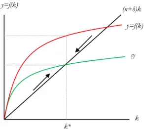
Three sources of economic growth are identified in traditional neoclassical growth; improvements in technology, increases in labor quantity and quality, and increases in capital (Todaro & Smith, 2006). A quantitative increase in labor would mean population growth, and a qualitative one means an increase in the education level. Increases in capital come through the savings used for investments. Disregarding technological progress, an economy is expected to reach a steady-state equilibrium level of output and capital per capita (Dornbusch, Fischer & Startz, 2008). The steady-state level is reached when the output per worker is constant, at point k* (where ) in Figure 3-1. Different countries have different steady-state levels of output and capital, depending in the neoclassical model on the propensity to save, population growth rate and productivity (Barro, 1997). At this steady state level, savings and investments are in balance, and the growth rate remains the same. An increase in savings will increase the level of GDP, since it results in a higher equilibrium value of k, but leave the growth rate unchanged, though in the transition process the higher saving rate increases the growth rate of output and output per head.

Figure 3-1 Solow‟s growth model

Solow (1956) expresses output as a function of capital and labor as follows:

where Y denotes national product, K is stock of capital, and L stock of labor. The neoclassical growth model thus can be expressed as a Cobb-Douglas function:

where Y, K and L are the same denotations as above, and A denotes level of technology (Romer, 1994). According to the model, per capita growth will eventually cease since the

k sy (n+δ)k y=f(k) y=f(k) k*

7

returns to capital will ultimately diminish completely. That A is a function of time alone illustrates the standard assumption that technological progress is taken as exogenous to the model, and is the counteracting force of the diminishing returns to capital.

Since capital is assumed to yield diminishing returns, states are expected to converge to the same income (Barro, 1997). Poor countries, with low capital to labor ratio, tend to have higher rates of return and thus higher growth rates. According to Barro (1997) this convergence property has been exaggerated, and mentions other phenomena in an economy that affects the growth rate, e.g. policies, propensity to have children, access to technology and willingness to work.

Mauro (1995) founds that there is a negative and significant relation between corruption and economic growth, but an even stronger one between corruption and investment. Though Leff (1964) asserts that corruption can increase the efficiency of burdensome bureaucracies through competition, Mauro (1995) finds the relationship to be true also in countries with very cumbersome bureaucracies and regardless of the amount of red tape. When measuring the effect of corruption on economic growth, one should not forget that institutions and economic variables evolve jointly – hence which one effect which is a matter of extent. Mauro (1995) further asserts that this negative relationship between corruption and economic growth in the neoclassical model comes through the misallocation of resources and production among sectors, thus affecting the steady-state level of income, and by decreasing the private marginal product of capital, lowering the investment rate.

3.2 Endogenous Growth Theory

Romer (1994) expresses five facts that theorists on economic growth traditionally have agreed upon. These are;

 Competition: economic activity is spread over many firms,

 Non-rivalry: discoveries differ from other inputs in that they are not excludable; they can be used by an infinite number of people at the same time,

 Replication: an even increase in the physical inputs results in an equal increase in output,

 Technology: progress in technology comes through things that people do, not merely by elapsed time,

 Monopoly: firms and individuals may possess market power and collect rents on discoveries,

out of which the neoclassical growth models accounts for the first three facts (Romer, 1994). The endogenous growth model therefore tries to accommodate at least the fourth fact, in an attempt to explain economic growth as dependent on factors endogenous to the economic system rather than on forces from the outside as in the neoclassical model (Romer, 1994). Instead of letting exogenous technological improvements explain the positive growth, the endogenous growth theory focuses on the development of technological knowledge and the forces in an economy that influences the incentives and opportunities to create such knowledge (The New Palgrave Dictionary of Economics). Or, as Ehrlich and Lui (1999) put it; human capital, and the investment therein, is the engine of growth in an economy.

8

The theory evolves in two stages, or waves. The first wave of endogenous growth theory, also called the AK-theory, emphasizes that the long run economic growth rate depends on the savings rate (physical capital accumulation) and education (knowledge accumulation) (Lucas, 1998). Thus

where Y is output, A is technology, and K is capital. In this first wave no distinction is made between the physical and human capital studied in neoclassical growth theory, and between the intellectual capital associated with innovations. Instead, constant or increasing returns to scale are assumed, as it is believed that some of the accumulation in capital will be intellectual capital, creating technological progress and offsetting the diminishing returns to capital. Long run growth is then determined by the savings rate, and if a fraction, s, of output is saved, and there is a fixed rate of depreciation, δ, then net investments are given by:

Which in turn implies that the growth rate, g, is given by:

An increase in the capital accumulation will therefore lead to a permanently higher growth rate.

A second wave, also called innovation-based theory, separates intellectual capital from physical and human capital, and growth comes through innovation rather than capital accumulation and education. According to Romer (1991) productivity increases along with the degree of product variety;

where 0< α<1, L denotes labor, x(i) the flow input of intermediate product i, and A is the amount of different varieties that are available. Thus, more varieties mean that the resources are spread between a larger number of production activities, and in the prevalence of diminishing returns the more varieties produced, the more efficiently are the resources allocated.

According to the Schumpeterian view however, innovation enhances the production by improving the quality of products, rather than the quantity. The output equation;

is reconstructed where now the product variety is a normalized fixed measure of unity and where a separate productivity parameter A(i) is coupled together with each intermediate product i. Innovations in products where the productivity parameter outmatches the previous parameter will lead to a supposable growth rate in A(i) of;

9

where the growth rate is dependent on the flow of innovation, μ, and a fixed factor, γ. The flow of innovation is proportionally linked together with the present flow in research and development (R&D).

R is the output spent on R&D and A takes into account the complexity of increased quality. By combining the last equations the growth rate is calculated by:

or, if the fraction of GDP spent on R&D is ;

Growth thus becomes a product based on the maximization of output, labor and the amount spent on R&D. Innovation-based theory suggests that as large of a fraction as possible should be spent on R&D, instead of on savings. The theory deals distinctively with the effects from policies on R&D activities and additionally how well the technological progresses in the society are handled.

Bureaucratic corruption is an inevitable feature of any government intervention in an economy since any intervention requires assignment of responsibility to bureaucrats, who then possess power to extract bribes (Ehrlich and Lui, 1999). This in turn creates an incentive for individuals to become a bureaucrat, with the privilege of collecting bribes, a phenomenon often referred to as rent-seeking. The cost of corruption then lies in that resources will be invested in such activities, rather than in accumulating human capital. Corruption could also enter the endogenous growth model through distortions in the educational system, e.g. through inequality in the access to education, in the distribution of educational materials, in the acquisition of educational goods and services, and through administrators and teachers in the system (Heyneman, 2004).

Murphy, Schleifer and Vishny (1993) make the argument that corruption reduces the returns of production, and if the fall in these returns is larger than the returns on corrupt and rent-seeking activities, resources will flow from productive activities to corrupt ones. Thus corrupt countries will end up with lower stocks of human capital and other factors of production.

Although the endogenous growth model provides possible explanations for long term growth, much of the cross-country empirical studies of economic growth still are influenced by the neoclassical model (Barro, 1997). The neoclassical model is then often extended with other variables such as government policies, human capital and dispersion of technology.

3.3 Related empirical studies

To determine GDP growth a number of variables have been found to be of significance. In examining the robustness of variables used in previous empirical studies, Levine and Renelt (1992) conclude that four variables are of importance. Those are the initial level of GDP, the education level, the average annual rate of population growth, and the investment share of GDP. These are all significant and robust in different tests performed. There is a negative correlation between GDP growth and the initial level of income, as supported by

10

previous literature and theories of conditional convergence; a poor country grows faster than a richer one, other things equal.

Levine and Renelt (1992) let the secondary-school enrollment rate be the measure of education. There is a robust and positive relationship between the education variable and the GDP growth rate. This is consistent with most previous research, where education is found to effect economic growth positively (e.g. Barro, 1991). Barro (1997) finds that an extra year of male schooling increases the magnitude of the convergence theory, which leads to the conclusion that education is important for the capacity to absorb new technologies in an economy.

Population growth measures increases in labor quantity. It is expected to be negatively correlated with economic growth, though Levine and Renelt (1992) find that the correlation is vague. In several tests a negative relationship is found, but in others the indicator turns out insignificant. Furthermore, a robust and positive relationship between GDP growth and the investment share of GDP is found. However, there is reason to question the causality of this relationship, as an economy with good growth opportunities is likely to attract investments, both domestic and foreign (Barro, 1997).

Levine and Renelt (1992) confirm the finding by Barro (1991) that a dummy for Latin American and Sub-Saharan African countries is significant. The dummy is based on the fact that both Latin American and Sub-Saharan countries have experienced unexpectedly low growth rates, and the dummy therefore tests if the growth is explained by factors exogenous to the model or explained by the included variables (Barro, 1997). An insignificant dummy means that the low growth rates in these countries are explained by the explanatory variables of the model. Barro (1997) finds that the dummy is not significant, neither a combined dummy for Latin America and sub-Saharan Africa nor separated ones.

In international trade theory, comparative advantage stand as the main explanation for why countries trade with each other. When focusing on the production for which an economy has a comparative advantage, and importing the remaining goods, resources such as capital and labor will be reallocated to where the production which uses the factor more intensely is situated (Krugman and Obstfeld, 2009). In this way all countries involved in the trade are expected to experience increases in economic growth. How open a country is to trade has therefore been considered as an important variable in growth equations. This openness of an economy, i.e. the total trade as a percentage of GDP, has turned out to be a significant variable when estimating GDP growth in an endogenous growth model, but rather insignificant when using a neoclassical growth model (Rivera-Batiz and Romer, 1991). When testing the robustness of different independent variables in economic growth regressions, Levine and Renelt (1992) states that the share of trade in GDP is positively correlated with the investment share of GDP, and thereforeus suggests that it controls for the same effect as the investment variable.

11

4 Model

The following model is used to test the relationship between corruption and economic growth:

The data included in the regression is drawn from the World Bank, UNESCO, and Transparency International.

GDP growth is treated as the dependent variable in the regression. It analyzes the growth in GDP from 2004 to 2008. The values are calculated based on country GDP data from the World Bank (2011) measured in constant 2000 U.S. dollars. GDP growth is included in percentage form.

The explanatory variables in the regression are initial GDP, population growth, education, openness, capital formation, and corruption. There is also a dummy variable included accounting for if the country belongs to Latin America or Sub-Saharan Africa. A value of 1 indicates that the country is located either in Latin America or Sub-Saharan Africa. The dummy variable is included based on previous findings that the low growth in these regions depend also on factors not accounted for in traditional growth equations, such as e.g. history, (Dreher et al., 2007). For this reason, the dummy variable is expected to be negative.

Levine and Renelt (1992) found that the most important variables to be held constant when testing the relationship between economic growth and any variable of interest are initial level of GDP, education, and average annual rate of population growth.

Initial GDP is drawn from the same sample as GDP growth. The values are from the base year 2004. The commonly known theories of convergence imply that the lower GDP level a country has, the more capability it has to grow. Based on this, a high level of initial GDP lowers the possibility of obtaining a high growth rate. Thus the expected value of the variable is negative.

The population growth variable is calculated from the total population data from the World Bank. Total population in a country includes all residents regardless of nationality or legal status, except for refugees and people of asylum. The values are mid-year estimates (World Bank, 2011). For the regression the population growth rate from 2004-2008 is calculated based on the population data. The variable is expected to have a negative coefficient, since when the population size increases, the available capital has to be distributed over a larger amount of workers.

Gross capital formation was formerly known as gross domestic investment. The data is calculated based on improvements on assets in the economy. It consists of the additions made on fixed assets throughout the year added together with the net change of inventories (World Bank, 2011). The calculated data in the regression is a mean of gross capital formation over 2004-2008, as a percentage of GDP.

12

The openness index is a measure of total trade as a percentage of GDP, i.e. the sum of exports and imports of goods and services divided by GDP (World Bank, 2011). In the regression analysis, data from 2004 from the World Bank is used.

For the education variable, gross secondary school enrollment rate has been used, as standard in the literature (Levine and Renelt, 1992). A mean over the years 2004-2008 is calculated. The gross enrollment ratio includes both lower and upper secondary enrollment (UNESCO, 2011). Education is assumed to be positively related with economic growth, as more stable government with low levels of corruption tend to spend more on education (Mauro, 1995).

For the corruption variable the Corruption Perception Index (CPI) given out by Transparency International, is used. It is a measure of the perceived levels of corruption in 180 countries, based on expert groups and surveys. The measure is a rank from 0,0-10,0, where a low value indicates high perceived corruption (Transparency International, 2011c). The CPI index in this thesis is a mean value of CPI values from 2004-2008. The corruption variable is expected to have a positive value. As CPI increases, perceived corruption decreases and GDP growth per capita is expected to increase.

Population growth, gross capital formation, openness index, and the education ratio are all measured in percentage, expressed in decimal form. For the variables education, capital formation, and CPI, mean values have been calculated and used in the regression. This has allowed for more observations to be included, since there are gaps in the collection of data through the observed years. The purpose is to use as big of a sample as possible. However, since some information is unavailable for some countries during these years, the countries have been excluded from the regression. The final sample size used in the regression is 123 observations (see Appendix 1A-1B).

As noted above, the final model used in the regression is:

13

Table 4-1 Variables

Variable Description Source Expected

outcome

Y GDP growth per capita

(2004-2008, %) World Bank Dependent variable

X1 Initial GDP per capita

(2004) World Bank -

X2 Population growth (Mean 2004-2008,

%) World Bank -

X3 Education

(Mean 2004-2008, %) UNESCO +

X4 Openness

(2004, %) World Bank +

X5 Gross capital formation (Mean

2004-2008, %) World Bank +

X6 Corruption Perception Index

(Mean 2004-2008) Transparency International +

D7 Dummy controlling for geographical

location -

14

5 Empirics

This section presents the results obtained from the regressions run on the model based on the previous section. It investigates if CPI affects the economic growth rates in the countries included in the sample. The analysis is carried out based on the theories elucidated in section 3.

5.1 Results of the estimated coefficients

The descriptive statistics on the sample is presented in Table 5-1.

Table 5-1 Descriptive statistics

Variable Mean Median Maximum Minimum Std. Dev.

Dependent:

GDP Growth per capita 17.079 14.670 59.939 -20.193 12.463

Independent:

Initial GDP per capita 7782.898 2359.459 50063.72 133.954 10957.84

Education 0.751 0.825 1.491 0.108 0.297 Openness 0.883 0.739 3.714 0.247 0.502 Dummy 0.414 0.000 1.000 0.000 0.495 Population Growth 0.053 0.050 0.146 -0.049 0.043 Capital Formation 0.238 0.224 0.443 0.089 0.062 CPI 4.333 3.400 9.500 1.760 2.196

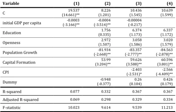
The authors have performed four different regressions on GDP growth. The results from the completed regressions are displayed in Table 5-2. The regressions are ordinary least square regressions, all of them treating the same 123 observations. The dependent variable is GDP growth per capita from 2004 to 2008 in percentage form. The analysis is based on regression 3 with additional analysis on regressions 1, 2, and 4.

The F-statistic for all four regressions is relatively high which indicates that at least one of the variables in every regression is significantly different from zero. The R-squared value for regression 1 is 0.367. Thus, almost 37% of the variance from the regression can be explained by the model. The adjusted R-squared value is 0.3288. Excluding the CPI variable as done in regression 2 will decrease the adjusted R-squared. Excluding the initial GDP per capita variable as done in regression 4 will give a higher adjusted R-squared implying the model is a better predictor.

15

Table 5-2 Regression output

Dependent variable GDP growth per capita (2004-2008)

Variable (1) (2) (3) (4)

C _(14.661)** 19.537 _(1.201) 8.226 _(1.545) 10.436 _(1.599) 10.639

initial GDP per capita _(-3.166)** -0.0003 _(-3.514)** -0.0004 -0.00004 _(-0.217)

Education _(0.335) 1.756 _(1.173) 6.374 _(1.172) 6.337 Openness _(1.507) 2.972 _(1.586) 3.058 _(1.579) 3.020 Population Growth _(-2.668)** -81.934 _(-2.777)** -83.357 _(-2.878)** -84.563 Capital Formation _(3.204)** 53.99 _(3.588)** 59.626 _(3.801)** 60.596 CPI _(-2.531)* -2.403 _(-4.409)** -2.566 Dummy _(-0.377) -0.948 _(0.104) 0.26 _(0.179) 0.426 R-squared 0.077 0.332 0.367 0.367 Adjusted R-squared 0.069 0.298 0.329 0.334 F-statistic 10.023 9.614 9.539 11.213 Notes: Number of observations: 123 * = p<0.05 ** = p<0.01

The CPI coefficient is contradicting the expectation of a positive value, and enters with a

negative correlation coefficient. It is statistically significant at the 5% level, implying that a 1 unit increase in CPI, i.e. a decrease in perceived corruption, will lower GDP growth per capita with 2.4 percentage points, other things equal. A scatter plot of the correlation is shown in Figure 5-1 where the relationship is relatively observable. A higher value of CPI, i.e. low corruption, implies a lower growth rate.

Figure 5-1 Scatter plot: CPI v. GDP growth per capita

-40 -20 0 20 40 60 80 1 2 3 4 5 6 7 8 9 10 CPI G D P g ro w th /c a p it a

16

Initial GDP per capita is negatively correlated with GDP growth per capita, but only

significant (at the 1% level) in the regressions that exclude the CPI variable. The latter finding indicating a correlation between the two independent variables, on which a more extensive analysis will be put forward in the discussion.

The gross capital formation variable is significant at 1% level in all regressions; it also has

the positive value as expected. A 1 unit increase in investments, representing an increase of 100 percentage points, will give an approximate increase in GDP growth per capita of 60 percentage points, other things equal.

Population growth is significant and negatively related to economic growth as expected.

When the population increases in a country, the GDP growth per capita decreases, other things equal. A 1 unit increase in population, again representing 100 percentage points, causes a decrease of approximately 80 percentage points in the growth, other things equal.

Openness is a measure of how freely trade flows in and out of a country. The coefficient

is positively related to GDP growth as expected, however it is insignificant at the 5% level in all three regressions.

The education level in a country is expected to be positively related to economic growth.

A higher level of education implies more skilled workers and a rise in the economic activity in a country. Even though the variable is positive in the regression, it is insignificant at the 5 % level.

The dummy included in regressions 2-4 was highly insignificant in all three regressions.

This implies that the growth rates in these countries can be explained by the model to the same extent as the other countries.

5.2 Other tests of the model

Tests for heteroscedasticity and multicollinearity are performed to draw the conclusion if the model is a good estimation. Instead, a test performed on the regression is White‟s General Heteroscedasticity Test.

The test hypothesis is:

The obtained chi-square value for regression 3 is 38.73618, found in Table 5-3. The critical chi-square value with a probability of 0.05 and 34 degrees of freedom is 48.602. Since [χ2_{obs = 38.73618] < [χ}2_{crit = 48.602], the null hypothesis cannot be rejected and the}

conclusion is that there is no significant heteroscedasticity in the regression.

Table 5-3 White‟s test

17

A second test is performed to evaluate whether multicollinearity is present. Multicollinearity exists if there is some degree of linear relationship between the regressors in a model. The regression becomes inefficient but unbiased. Tests for multicollinearity can be conducted by calculating the variance-inflating factor (VIF). The VIF for regression 3 is 1.580638. Analyzing the individual VIFs in Table 5-4 between the variables against GDP per capita will generate values close to 1 which indicates that multicollinearity is not a severe problem in the model, as explained by Gujarati and Porter (2009).

Table 5-4 VIF VIF GDP growth/capita - Initial GDP/capita 1.082843 Education 1.007363 Openness 1.019475 Dummy 1.018955 Population growth 1.128477 Capital formation 1.208611 CPI 1.071297 Regression model (3) 1.580638

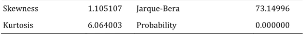
A normality test is performed to analyze the normality of the disturbance term. Two tests were carried out, as suggested in the book by Gujarati and Porter (2009). The results, presented in Table 5-5 show that the residuals are not normally distributed. The skewness and the kurtosis should be zero and three respectively and the Jarque-Bera statistic should be as low as possible. The result indicates that the model may contain misleading information about the dependent variable.

Table 5-5 Normality test

Skewness 1.105107 Jarque-Bera 73.14996

Kurtosis 6.064003 Probability 0.000000

5.3 Discussion

In order to evaluate whether perceived levels of corruption affect economic growth rates as stated in the research question a test hypothesis was constructed. The test hypothesis is:

If the null hypothesis cannot be rejected CPI can be excluded from the model. The t-value for the variable is approximately -2.53 (found in Table 5-2) and significantly different from

18

zero at p<0.05. Thus can the null hypothesis be rejected and the result shows that CPI affects economic growth rates.

Even though there is a relationship, the CPI coefficient is negative, contradicting the expectation derived from previous research. Since it is statistically significant at a 5% level, this implies that a 1 unit increase in CPI, i.e. a decrease in perceived corruption, will lower GDP growth per capita with 2.4 percentage points. The authors want to argue that this does not have to prove that economic growth benefits from corruption, but rather that there are other factors behind this result.

If it is assumed that corruption affects investments in a negative way, as found by Mauro (1995), this should affect the growth rate in the same direction. In the regression above, the gross capital formation share of GDP is positive and significant which is consistent with the neoclassical theory. In the neoclassical growth theory, the level of investment is crucial for an economy to increase its GDP level. If the savings made in a country are invested abroad rather than domestically, the country will have a low capital to labor ratio, k*, showed in Figure 3-1, and thus a low output to labor ratio.

So, if corruption is prevalent and impacts the level of the investments negatively, it should be detrimental to the equilibrium level of capital and output per worker (Dornbusch et.al. 2008). However, in the regression of this thesis no correlation is found between capital formation and corruption, contrary to what Mauro found (1995). Even so, it is perhaps most probable that corruption does in fact affect investments, but it cannot be proved for this period of time with the data used in the regression. Or, as Bardhan (1997) suggests, the perception of the existence of corruption might differ between foreign investors and the domestically questioned people that are the basis for the index. Thus implying that both the actual and the domestically perceived level of corruption might be somewhat irrelevant in determining the amount of foreign capital invested.

It could also be that the investments are made in spite of the corruption, as the investors expect the returns on the investments to be larger than the cost of the bribes they will have pay. It is however unclear from the regression in which direction the causality goes; does a higher level of investment increase the growth rate, or does the high growth rate attract investment?

The investments needed depend on the growth rate of the population and the rate of depreciation of capital. So if the population grows faster than new capital is accumulated, the steady state level falls. As is thus expected, the population growth variable has a negative sign, since growth per capita is measured and not aggregate growth.

As stated above, the corruption variable has a negative coefficient in the regression, and since the level of corruption decreases as the scale of the index ascends, this means that the more corruption that has been perceived in a country, the higher growth rate it has experienced. The initial GDP per capita variable is only significant in the regressions that exclude this negative impact of the CPI variable. It is then negatively correlated with GDP growth per capita, which confirms the theory of conditional convergence. A possible, and likely, explanation of the insignificance of initial GDP when CPI is included is the high correlation between the two. The correlation coefficient amounts to almost 0.9 (see Appendix 2A). Below is a scatter plot of the relationship between the two variables (Figure 5-2). From this it can be seen that there in fact is a relation between the variables;

19

corruption is more prevalent in countries with lower levels of GDP per capita. Thus, in general, poor countries are more corrupt.

Figure 5-2 Scatterplot: CPI v. Initial GDP per capita

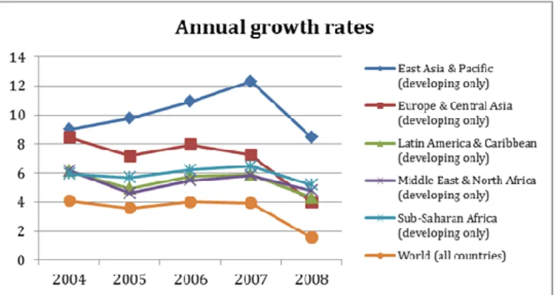
From the data used in the regression a graph was constructed to show how the growth rates in developing countries have been higher than the world average, see Figure 5-3.

Figure 5-3 Annual growth rates 2004-2008

In this graph it can be seen that the developing countries in all regions have experienced higher growth on average, than the total world on average, in line with Solow‟s theory of conditional convergence. As poorer countries are generally abundant in natural resources (Sachs and Warner, 2001), their economic growth relies in large part on this sector of the economy. Sachs and Warner (2001), among others, show that there is a strong relationship between this resource abundance and the low growth rates experienced in these countries since the 1970‟s. Thus the unusually high growth rates shown in the graph above, can perhaps be explained by the high prices of natural resource commodities during these years, as exemplified by the rise in gasoline prices from 1.200SUSD per gallon in 2001 to 3.069USD per gallon in 2007 (Bureau of Labor Statistics).

0 10,000 20,000 30,000 40,000 50,000 60,000 1 2 3 4 5 6 7 8 9 10 CPI in it ia l G D P /c a p it a

20

Economic growth is positively affected by the investment to GDP ratio, as seen in the regression. Looking at the scatterplot of capital formation against initial GDP in Figure 5-4, it shows that the levels of investments seem to be rather even in countries with an initial GDP per capita of above approximately 10,000 constant 2000 USD, but when the countries have had lower levels of GDP than that, the level of investment varies extremely; both the lows and the highs are found within the poorest countries. The explanation for this needs to be searched for outside the model constructed in this thesis, but it is clear from this plot that only a low level of initial GDP has not been reason enough to attract capital.

Figure 5-4 Scatterplot: Initial GDP per capita v. Capital formation

It seems however that the investment potential in these poorer countries have been a stronger force in attracting capital during the years 2004 to 2008, than the level of corruption perceived, in repelling it. This would imply that the economic convergence has a stronger effect on the economy than the corruption has, and since investments are not affected by corruption, as stated above, corruption does not affect the economic growth in the neoclassical model.

Obviously investments are made in spite of the perceived level of corruption, which is likely explained by that the expected return on these investments are high enough to offset the cost of the bribes and the uncertainty associated with a corrupt environment. If the investors are aware of these costs, it seems that they calculate the benefit of investing in a developing, albeit corrupt, country to exceed these costs. It is however unclear from the regression in which direction the causality goes; does a higher level of investment increase the growth rate, or does the high growth rate attract investment?

That there is a correlation between initial GDP and corruption is further confirmed by a comparison of the regressions: excluding the initial GDP per capita variable generates a stronger CPI variable in regression 4 that is significant at 1% level. Running a regression without the CPI variable will result in a significant initial GDP per capita variable (regression 2). A regression solely including initial GDP per capita as explanatory variable (regression 1) will give a model where the constant and the slope are statistically different from zero a 1% level.

.05 .10 .15 .20 .25 .30 .35 .40 .45 0 10,000 20,000 30,000 40,000 50,000 60,000 initial GDP/capita C a p it a l fo rm a ti o n

21

As mentioned earlier, Levine and Renelt (1992) find that there is positive relationship between the share of trade in GDP and the share of investment in GDP. When both of the variables are included in a growth equation, the trade variable ends up insignificant, despite the fact that both variables are significant when tested alone. The conclusion is that the positive effects of trade on growth works through investments, i.e. enhanced resource accumulation, rather than enhanced resource allocation. The latter being the traditional argument for why trade increases economic growth. In the regressions of this thesis, the trade variable does indeed turn out insignificant. However, in the same regressions, the correlation between this variable and the investment variable, capital formation, is weak, around 0.16 (showed in Appendix 2A). Thus it seems that neither the argument that trade affects growth through resource accumulation, nor the traditional argument that it increases growth through resource reallocation, seem to hold for this period of time. In contrast to the previous research mentioned earlier, economic growth seems unaffected by the secondary school enrollment rate; the variable for education turns out to be insignificant during this period of time. There is thus no linear relationship between education and GDP growth. Most likely, this does not imply that the level of education is not an important determinant of economic growth, most empirical studies say otherwise; a higher level of education implies more skilled workers and thus a higher level of productivity. It is more probable that this effect has been hidden by other variables in the regressions, or the variable for secondary school enrollment rate is not an accurate estimation of the education level. A suggestion would be to instead include a variable accounting for the expenditures on higher education or R&D.

Barro (1997) argues that a high level education enhances the possibilities to take advantage of new technologies. This would then mean that a country with a high level of corruption, and thus lower levels of education, would struggle more to absorb new technologies. This in turn hurts productivity and economic growth.

Even if education does not seem to affect economic growth in the above regressions, there is a relationship between the education variable and CPI; the variables have a correlation of 0.66 (see Appendix 2A). When looking at a scatterplot of this relationship (see Appendix 3A) it appears that when corruption falls below a certain level (above ~3 in the CPI), there is a strong positive linear relation, but above this level of corruption this linear correlation is non-existent. Thus it appears that in corrupt countries the level of education is trapped at a low to intermediate level, but as soon as corruption starts to decrease, the educational level takes off. However, this relationship is most probably explained by the variables‟ mutual relation to level of GDP per capita.

The dummy included in regressions 2-4 was highly insignificant in all three regressions. This implies that the growth rates in these countries can be explained by the model to the same extent as the other countries.

22

6 Conclusion

The purpose of this thesis was to test if the level of perceived corruption in a country is correlated to its rate of economic growth. Most literature and previous studies find that it should be, and that this relation should be negative. This was thus the expected result. To test this, four regressions were conducted. The Corruption Perception Index was used as the variable accounting for corruption, and an additional number of control variables, standard in the literature, were also included.

The results were somewhat divergent from the predictions made based on theory and previous research; in the regressions of this thesis, corruption increases economic growth instead of lowering it. The authors are however reluctant to conclude that corruption contributes positively to growth. Instead, by comparing the results of the different regressions, looking at the scatter plot, and taking note of the correlation matrix in Appendix 2A, it is found that there is a correlation between the corruption variable and the level of initial GDP. This correlation is negative; the lower the level of corruption the higher the level of initial GDP and vice versa. Noting that developing countries, with lower levels of initial GDP per capita, have in general had higher annual growth rates over the years 2004-2008 than the rest of the world, the authors assume that some other force is driving the development, and corruption is not a strong enough force to counteract it. Perhaps is corruption detrimental to growth, even though it cannot be shown in a macro study like this one. For instance it could work through education, a variable to which corruption has a negative linear relationship below a certain level. If a country has low to intermediate levels of education it seems corruption prevails at a low level, whilst when education starts to increase, the corruption level falls.

Furthermore, previous studies have found that corruption can lower economic growth through its effect on investments. No such relationship was however found in this thesis. Investment is however found to be significant in explaining growth. Openness is found to be insignificant. This despite the fact that its correlation to capital formation is weak, a phenomenon often used to explain insignificance of trade variables. A dummy was introduced with the purpose of distinguishing countries in Latin America and Sub-Saharan Africa from the rest of the world since there seem to be some yet undetermined factors affecting the growth rates in these countries. However this dummy variable turned out insignificant, and the growth in this countries can thus be measured by the model to the same extent as other countries.

Micro studies on the effect of corruption have been done, showing a robust relationship between the existence of corruption and the effects on regional levels. Perhaps a macro study like the one conducted here is too broad in order to prove the negative effects of corruption. Despite this, the authors are still convinced that low levels of corruption are desirable for countries in order to achieve sustainable growth.

23

References

Acemoglou D., & Verdier, T. (1998). Property rights, corruption, and the allocation of talent: a general equilibrium approach. Economic Journal, 108(450), 1381-1403.

Andersson, S., & Heywood, P. M. (2009). The Politics of Perception: Use and Abuse or Transparency International‟s Approach to Measuring Corruption. Political Studies,

57(4), 746-767.

Bardhan, P. (1997). Corruption and Development: A Review of Issues. Journal of Economic

Literature, XXXV(3), 1320-1346.

Barro, R. J. (1991). Economic growth in a cross section of countries. The Quarterly Journal of

Economics, 106(2), 407-443.

Barro, R.J. (1997). Determinants of economic growth: a cross-country empirical study. Cambridge: The MIT Press.

Brown, S. F., & Shackman, J. (2007). Corruption and Related Socioeconomic Factors: A Time Series Study. Kyklos, 60(3), 319-347.

Bureau of Labor Statistics (2011). Databases, Tables and Calculators. Retrieved June 2, 2011 from http://data.bls.gov/pdq/SurveyOutputServlet

Dornbusch, R., Fischer, S., & Startz, R. (2008). Macroeconomics (10th _{edition). New York:}

McGraw-Hill.

Dreher, A., Kotsogiannis, C., & McCorriston, S. (2007). Corruption Around The World: Evidence From A Structural Model. Journal of Comparative Economics, 35(3), 443-466. Ehrlich, I., & Lui, F.T. (1999). Bureaucratic Corruption and Endogenous Economic

Growth. The Journal of Political Economy, 107(6), 270-293.

Easterly, W. (2001). The Lost Decades: Developing Countries‟ Stagnation in Spite of Policy Reform 1980-1998. Journal of Economic Growth, 6(2), 135-157.

Global Issues (2010). Poverty Facts and Stats. Retrieved April 20, 2011 from http://www.globalissues.org/article/26/poverty-facts-and-stats#src1

Gujarati, D. N., & Porter, D. C. (2009). Basic Econometrics (5th _{edition). Boston:}

McGraw-Hill.

Gyimah-Brempong, K. (2002). Corruption, economic growth, and income inequality in Africa. Economics of Governance, 3(3), 183-209.

Heyneman, S.P. (2004). Education and Corruption. International Journal of Educational

Development, 24(6). 637-648.

Howitt, P. (2008).Endogenous growth theory. The New Palgrave Dictionary of Economics. 2nd _{ed. Durlauf, S. N. & Blume L. E. (Eds.). The New Palgrave}

Dictionary of Economics Online. Palgrave Macmillan. Retrieved March 4, 2011 from http://www.dictionaryofeconomics.com/article?id=pde2008_E000079

24

Husted, B. W. (1999). Wealth, culture and corruption. Journal of International Business Studies,

30(2), 339-359.

International Monetary Fund (2010). Database—WEO Groups and Aggregates Information. Retrieved April 20, 2011 from

http://www.imf.org/external/pubs/ft/weo/2010/01/weodata/groups.htm#oem Jain, A. K. (2001). Corruption: A review. Journal of Economic Surbeys, 15(1), 71-121.

Leff, N. (1964). Economic Development Through Bureaucratic Corruption. American

Behavioral Scientist, 8(3), 8-14.

Levine, R., & Renelt D. (1992). A Sensitivity Analysis of Cross-Country Growth Regressions. The American Economic Review, 82(4), 942.963.

Lucas, R.E. Jr. (1988). On the Mechanics of Economic Development. Journal of Monetary

Economics, 22(1), 3-42.

Lui, F. T. (1985). An equilibrium queuing model of bribery. Journal of Political Economy, 93(4), 760-781.

Mankiw, N.G., Romer, D., & Weil, D.N. (1992). A contribution to the empirics of economic growth. The Quarterly Journal of Economics, 107(2), 407-437.

de Maria, B. (2008). Neo-colonialism through measurement: a critique of the corruption perception index. Critical Perspectives on International Business, 4(2/3), 184-202.

Mauro, P. (1995). Corruption and Growth. The Quarterly Journal of Economics, 110(3), 681-712.

Mauro, P. (1997). The effects of corruption on growth, investment and government expenditure: a cross-country analysis. In K. A. Elliott (Ed), Corruption and the global

economy (pp. 83-107). Washington, DC: Institute for International Economics.

Mo, P. H. (2001). Corruption and economic growth. Journal of Comparative Economics, 29(1), 66-79.

Mocan, N. (2004). What determines corruption? International evidence from micro data. Working paper 10460. NBER.

Philp, M. (2006). Corruption Definition and Measurement. In C. J. G. Sampford, A. Shacklock, C. Connors & F. Galtung (Eds.), Measuring Corruption (pp. 45-56). Aldershot: Ashgate Publishing Limited.

Rivera-Batiz, L.A. & Romer, P.M. (1991). Economic Integration and Endogenous Growth.

The Quarterly Journal of Economics, 106(2), 531-555.

Romer, P. M. (1994). The origins of endogenous growth. The Journal of Economic Perspectives,

8(1), 3-22.

Rose-Ackerman, S. (1997). The Political Economy of Corruption. In K.A. Elliot (Ed.),

Corruption and the Global Economy (p. 32-60). Washington: Institute for International

25

Sachs, J.D., & Warner, A.M. (2001). Natural Resources and Economic Development: The Curse of Natural Resources. European Economic Review, 45, 827-838.

Shleifer, A., & Vishny R. W. (1993). Corruption. The Quarterly Journal of Economics, 108(3), 599-617.

Solow, R. (1956). A Contribution to the Theory of Economic Growth. The Quarterly Journal

of Economics, 70(1), 65-94.

Svensson, J. (2005). Eight Questions about Corruption. Journal of Economic Perspectives, 19(3), 19-42.

Todaro, M.P., & Smith, S.C. (2006). Economic Development. Harlow: Pearson/Addison Welsey.

Transparency International (2011a). Corruption Perceptions Index. Retrieved April 20, 2011, from http://www.transparency.org/policy_research/surveys_indices/cpi

Transparency International (2011b). Frequently asked questions. Retrieved March 3, 2011, from

http://www.transparency.org/policy_research/surveys_indices/cpi/2007/faq#gener al1

Transparency International (2011c). Frequently asked questions about corruption. Retrieved March 3, 2011, from http://www.transparency.org/news_room/faq/corruption_faq Treisman, D. (2000). The Causes of Corruption: A cross-national study. Journal of Public

Economics, 76(3), 399-457.

UNESCO (2011). Table 5: Enrolment ratios by ISCED level. Retrieved March 30, 2011 from http://stats.uis.unesco.org/unesco/ReportFolders/ReportFolders.aspx

United Nations. (2006, June 28). Press release ORG/1469: United Nations Member States. Retrieved April 20, 2011 from

http://www.un.org/News/Press/docs/2006/org1469.doc.htm

United Nations. (2010). The Millennium Development Goals Report. Retrieved April 20, 2011 from

http://www.un.org/millenniumgoals/pdf/MDG%20Report%202010%20En%20r1 5%20-low%20res%2020100615%20-.pdf

World Bank (2011). World Development Indicators. Retrieved March 21, 2011 from http://data.worldbank.org/indicator

26

Appendix 1

Appendix 1A Countries outside Latin America and Sub-Sarahan Africa

Albania Algeria Armenia Australia Austria Bangladesh Belarus Belgium

Bosnia and Herzegovina Bulgaria Cambodia Canada China Croatia Cyprus Czech Republic Denmark

Egypt, Arab Rep. Estonia

Finland France Germany Greece

Hong Kong SAR, China

Hungary Iceland India Indonesia

Iran, Islamic Rep. Ireland Israel Italy Japan Jordan Kazakhstan Kyrgyz Republic Lao PDR Latvia Lebanon Lithuania Luxembourg Macao SAR, China Malaysia Maldives Moldova Morocco Netherlands New Zealand Norway Pakistan Philippines Poland Portugal Romania Russian Federation Saudi Arabia Serbia Slovak Republic Slovenia Spain Sweden Switzerland

Syrian Arab Republic Tajikistan

Thailand Tunisia Turkey Ukraine

United Arab Emirates United Kingdom United States Uzbekistan