www.transportekonomi.org
Long-term responses to car-tax policies: Distributional
effects and reduced carbon emissions
Roger Pyddoke, VTI
Jan-Erik Swärdh, VTI
Staffan Algers, TP mod AB
Shiva Habibi, Chalmers
Noor
Sedehi Zadeh, VTI
Working Papers in Transport Economics 2019:4
Abstract
We analyze the long-term effects on the car fleet and welfare distribution of three car-related policy instruments intended to reduce CO2 emissions: increased fossil-fuel taxes, an
intensified bonus-malus system for new cars, and increased mandated biofuel blending. The effects on the car fleet are analyzed in terms of energy source, weight, and CO2 emissions. Distributional effects are analyzed in terms of income and geographical residence areas. The increased fuel taxes reduce CO2 emissions by 36%, mainly through less driving of fossil-fuel cars. The intensified bonus-malus system for new cars reduces CO2 emissions by 5%. Both these policies shift the car fleet toward increased shares of electric vehicles and increased average weight. Increased mandated biofuel blending has no estimated effect on the car fleet unless prices increase differently from in the reference scenario. The two first policy
instruments are weakly progressive to slightly regressive over most of the income
distribution, but barely regressive if the highest income group is also included. The fraction of each population group incurring substantial welfare losses is higher the lower the income group. In the geographical dimension, for all policies the rural areas bear the largest burden, small cities the second largest burden, and large cities the smallest burden. The burden in the long term versus the short term is lower for high-income earners and urban residents. Keywords
Distributional effects, Equity, Fuel tax, Feebate, Bonus, Malus, Mandated biofuel blend, Car choice
JEL Codes D63, H23, R48
1
Long-term responses to car-tax policies: Distributional effects and
reduced carbon emissions
Roger Pyddoke*,^, Jan-Erik Swärdh*, Staffan Algers#, Shiva Habibi¤ and Noor Sedehi Zadeh* * VTI – the Swedish National Road and Transport Research Institute, Box 55685, 10215 Stockholm,
Sweden
# TP mod AB, Ringstedsgatan 63, 16448 Stockholm, Sweden
¤ Chalmers University, Department of Space, Earth and Environment, Physical Resource Theory, 412 96 Göteborg, Sweden
^ Corresponding author: roger.pyddoke@vti.se, +46 8 555 770 30
ABSTRACT
We analyze the long-term effects on the car fleet and welfare distribution of three car-related policy instruments intended to reduce CO2 emissions: increased fossil-fuel taxes, an intensified bonus-malus system for new cars, and increased mandated biofuel blending. The effects on the car fleet are analyzed in terms of energy source, weight, and CO2 emissions. Distributional effects are analyzed in terms of income and geographical residence areas. The increased fuel taxes reduce CO2 emissions by 36%, mainly through less driving of fossil-fuel cars. The intensified bonus-malus system for new cars reduces CO2 emissions by 5%. Both these policies shift the car fleet toward increased shares of electric vehicles and increased average weight. Increased mandated biofuel blending has no
estimated effect on the car fleet unless prices increase differently from in the reference scenario. The two first policy instruments are weakly progressive to slightly regressive over most of the income distribution, but barely regressive if the highest income group is also included. The fraction of each population group incurring substantial welfare losses is higher the lower the income group. In the geographical dimension, for all policies the rural areas bear the largest burden, small cities the second largest burden, and large cities the smallest burden. The burden in the long term versus the short term is lower for high-income earners and urban residents.
Keywords
: Distributional effects, Equity, Fuel tax, Feebate, Bonus, Malus, Mandated biofuel blend, Car choice2
1. Introduction
Reducing CO2 emissions from car traffic is central to the necessary policies for achieving international and national goals for emission reduction. Fuel taxes, bonuses and maluses payable for new cars, and mandated biofuel blending all constitute potential parts of such strategies. Although carbon taxes are attractive from an economic efficiency perspective, increases of such taxes are controversial for unfairly burdening rural inhabitants. The distributional concerns therefore emerge as an important obstacle to increased carbon taxes. As the potential burdens of climate policy become apparent, the issue of acceptability will also be a concern for policy makers (e.g. Carattini et al., 2019). Other measures to reduce carbon emissions are therefore also being considered, such as bonus-malus1 systems and mandated biofuel blending. There are also suggested policies intended to compensate groups particularly burdened by such policies. This calls for more careful analysis of the short- and long-term distributional consequences of such policy instruments.
Eliasson et al. (2018) analyzed the short-term distributional effects of different fuel and car taxes in the Swedish context using a fixed car fleet, finding that these taxes are slightly regressive and affect people in rural areas more than urban residents. Important policies target future car fleets, intended to speed up the introduction of carbon-free technologies such as electric cars or technologies, such as electric hybrids, that can substantially reduce carbon emissions. Therefore, the issue of long-term distributional consequences will be critical for the success of initiatives to incentivize greener car fleets.
This paper analyzes the potential long-term effects on the car fleet and welfare distribution by income and geographical residential areas of three different policy scenarios intended to decrease CO2 emissions up to year 2030. To analyze these effects on the private car fleet, we combine two previously used methods, the Swedish car fleet model (developed in 2006 and refined and updated several times, e.g. Transek, 2006; Hugosson et al., 2016; Habibi et al., 2019) and data from Swedish administrative registers on all Swedish adults and privately owned cars used by Eliasson et al. (2018). This is done by projecting the development of the car fleet in four different scenarios. A reference scenario uses the assumptions of official national forecasts made by the Swedish Transport Administration (2018) with all relevant policies in place in 2017. This reference scenario is used to compare how three policy scenarios affect the welfare of groups of individual adults in disposable income octiles and three geographical area types. The three policy scenarios involve increasing fuel prices by 50% (though increased taxation) starting in 2020, an intensified bonus-malus system
3
implying a higher tax on cars with emissions initially above 95 grams of CO2 per kilometer, also starting in 2020, and finally, a larger degree of mandated biofuel blending into gasoline and diesel. Three important strands of literature contribute to such an analysis. The first strand, focusing on the short-term (and sometimes longer-term) distributional effects of fuel taxes (cf. Eliasson et al., 2018), is the most extensive. Eliasson et al. (2018) find fuel taxation to be progressive over most of the income distribution but barely regressive if the highest and lowest income octiles are also included. Sterner (2012a, 2012b), reporting on fuel taxation in over two dozen countries, finds slight
regressivity in high-income countries, but mostly progressive effects in low-income countries. Fewer articles study distributional effects in terms of geographic dimensions as well. Examples include Bureau (2011), who finds larger welfare losses in rural than urban areas in France, Spiller et al. (2017), also accounting for car choices, who find the same difference in the USA, and Filippini and Heimisch (2016), who find the same difference in Switzerland. A recent contribution by Chatterton et al. (2018) finds larger expenditures in rural areas and indications of strong regressivity in the UK. In the second strand, the effects of policy on the short- and long-term adaptation of the supply and demand of new cars to various policy instruments are estimated using time series data. Examples of papers from this strand are by Huse and Lucinda (2013), Klier and Linn (2015), Bento et al. (2018b), and Grigolon et al. (2018), though these papers do not consider distributional issues. Huse and Lucinda (2013) analyze previous green car rebates in Sweden, finding that these rebates reduced the annual vehicle taxes on “green cars”. Estimations of counterfactual scenarios indicate that the rebates stimulated larger acquisitions of cars classified as green. Results also indicate that consumers would have acquired flexible-fuel cars even without the rebate. Klier and Linn (2015) estimate the effects of introducing annual carbon emission-based taxes on cars on the market shares of different car types in France, Germany, and Sweden. In France, the effects are fewer registrations of high-fuel-consuming cars; these effects are large and significant in the short term, while the long-term effects are smaller. A smaller effect is found in Germany, and the magnitude of the effect varies with estimation technique. In Sweden, the effects are indistinguishable from the effects of other trends. Grigolon et al. (2018) examine car buyer valuations of future fuel economy. They find only modest undervaluation of future fuel costs and conclude that although myopia may exist, fuel taxes are still the most effective policy for influencing car choice.
Bento et al. (2018b) review recent attempts to estimate the net social benefits of U.S. fuel efficiency standards by U.S. authorities (i.e. the Environmental Protection Agency and the National Highway Traffic Safety Administration), criticizing them for not using the best available methodologies. Their main argument is that when estimating the total effects on driving and carbon emissions, it is critical
4
to model interactions between the new and used vehicle markets. This point is elaborated on by Jacobsen and van Benthem (2015) and Bento et al. (2018a), who find strong effects of higher new car prices, which increase the demand for used vehicles and delay scrapping. Earlier, Bento et al. (2009) studied the distributional effects of U.S. gasoline taxes, also modeling the long-term effects on car choice.
The third strand uses discrete choice modeling of car choice, so-called car fleet models, to predict behavioral responses to future policy changes (for reviews of car fleet models, see e.g. Potoglou and Kanaroglou, 2008; Anowar et al., 2014). The Swedish car fleet model system has been used in several policy evaluations, i.e. Hugosson et al. (2016), Engström et al. (2019) and Habibi et al. (2019). In addition to these studies, several other papers have attempted to use discrete choice models to evaluate past policies by comparing them with counterfactual scenarios. There are several further examples of the discrete choice modeling of car fleets: Rasmussen and Strøm (2012) estimate how registration fees affect new car sales, finding that a bonus-malus scheme contributes to reduced CO2 emissions per kilometer; Adamou et al. (2011), studying the German bonus-malus scheme,
demonstrate the importance of having a well-defined starting point; and Brand et al. (2013) show that car purchase tax and feebate policies can be more effective in accelerating the uptake of low-emission vehicles than can road taxes and scrappage incentives in the UK. Other such studies are by, for example, Potoglou and Kanaroglou (2007), Mabit and Fosgerau (2011), and Mabit (2014). Unlike earlier analyses by, for example, Bureau (2011), Filippini and Heimisch (2016), Spiller et al. (2017), and Eliasson et al. (2018), who model distributional effects without the long-term adaptation of car ownership, the present paper considers the long-term effects of the adaptation of car
ownership to policy changes. The main contribution of this paper is to demonstrate the possible long-term effects of fuel taxes, bonus-malus schemes, and mandated biofuel shares on the private car fleet, carbon emissions, and welfare costs and distribution.
The remainder of this paper is organized as follows. Section 2 presents the data and methodology used. Section 3 presents the three policy scenarios, while section 4 presents the results in terms of effects on the car fleet and welfare distribution. Section 5 discusses the results and section 6 concludes the paper.
2. Data and methodology
2.1 Data
Data on individuals come from Statistics Sweden registers and data on cars come from the Swedish vehicle register, which covers all adults and all privately owned cars in Sweden. These data are described by Eliasson et al. (2018), but the available data have been expanded from 2011 to 2016.
5
Cars are linked to their registered owners through encrypted individual codes provided by Statistics Sweden.
The main advantage of using register data, besides the fact that they cover the entire population, is that they allow us to study small population segments in detail, in particular, detailed geographical segments. The main limitation is that we do not have access to household data, only data about the registered car owners. This could be a source of error if one wanted to explore variability in car use. For example, a household with two adults and one car used by both adults would appear in the register data as one individual with car use and one individual with no car use. This could be a limitation for the income analysis but will play no role in our geographical analysis.
In total, the population data cover 8.26 million adults living in Sweden in 2016, of whom 3.99 million live in large cities, 2.23 million in small cities, and 1.71 million in rural areas. In addition, the data record individual information such as disposable income, age, gender, residential location, and employment status.
The geographical residence areas are defined as follows. An “urban area” is a contiguous area where distances between houses do not exceed 200 m and the total number of inhabitants in the area exceeds 3000, including a further zone defined by a maximum car drive of 5 min to the contiguous area. Non-urban areas are defined as “rural”. “Large cities” are defined as urban areas in the three major metropolitan regions (i.e. greater Stockholm, greater Gothenburg, and greater Malmö) and in municipalities where the largest city has at least 60,000 inhabitants. “Small cities” are the remaining urban areas.
Vehicle data cover 5.34 million privately owned cars distributed over 3.69 million individual car owners. We have access to yearly vehicle kilometers taken from vehicle inspection data. Other car characteristics used are age, fuel type, fuel consumption, and weight.
Some exclusions from the data are necessary before the analysis. First, about 33,000 individuals could not be assigned to geographical residence areas and were excluded. Second, we excluded deregistered cars and cars weighing over 3500 kilograms. Third, individuals who own over four cars were excluded because it is unlikely that these cars are used only by their registered owners. The limit of a maximum of four cars is somewhat arbitrary but excludes few car owners, so this criterion is unlikely to distort the results (especially as the individual with the most cars in fact is registered as owning 3500 cars). In total, about 50,000 individuals and 980,000 cars (over 640,000 of which are not registered for use) are excluded for the above reasons. We end up with about 4.36 million privately owned cars distributed over about 3.47 million car owners.
6
The car fleet model is estimated using data from a survey of new car purchases conducted in 2014. The model is also calibrated to purchase data from 2017.
2.2 Methodology
In this project, we intend to identify how different car policies affect distribution of welfare. This entails understanding how different policies affect car purchases as well as how income distribution is influenced by costs, including subsidies, taxes, and fuel costs resulting from the car purchase and subsequent car use. Ideally, we should have a car fleet model with high resolution of socioeconomic variables, including mechanisms for reallocating used cars over time. In the absence of such a model, we use an existing car fleet model recognizing three different consumer segments to predict car purchases and that propagates the car fleet over time in terms of total car ownership and scrapping. The result of this model, which is sensitive to car policies, is a distribution of all personal vehicles by fuel type, model year, and average fuel consumption. This result has low resolution with respect to distributional variables. We therefore use an additional method to connect the car fleet results to private car owners and distributional variables. These models and methods are described in more detail below.
2.2.1 The Swedish car fleet model
The main structure of the Swedish car fleet model is described by Hugosson et al. (2016). The model contains three sub-models. The first sub-model is a scrapping model in the form of constant
scrapping rates by car age. The second sub-model is a model of the total number of cars in the car fleet, usually given by a long-term car ownership model. The number of new cars is given by the difference between the total number of cars in year t + 1 minus the total number of cars in year t after scrapping. The third sub-model is a model of the choice of car type for the new cars bought in year t + 1, describing the distribution of different types of new cars added to the car fleet of year t after scrapping. This is repeated for each year in the forecasting period. The car fleet is defined by model year and fuel type.
The car type choice sub-model is of course vital to the car fleet model, giving the market response to the different investigated car policies. This model has been updated in the current version of the Swedish car fleet model using data from 2014 in a survey carried out in 2015. The car choice sub-model covers three consumer segments: private buyers and company buyers with and company buyers without leasing arrangements. An important segment is cars provided by companies to employees for private use (here called benefit cars). We use the information on leasing arrangements included in the Swedish transport register as a proxy for this segment type. The estimation of models for the private and benefit car segments is described by Engström et al. (2019).
7
The estimation of the car type choice sub-model for the third segment is described by Hugosson et al. (2018).
The estimation of the car choice sub-model resulted in a number of statistically significant
parameters of car attributes, such as price, running cost (including taxes), size, range, NCAP safety class, and rust guarantee. The model is calibrated to the 2017 situation, using data from the national car register on new sales in 2017. The calibration consists of adjusting model constants for make and fuel type in the new car choice sub-models for each of the three consumer segments. The model parameters for the different explanatory variables are unaffected by this procedure, which results in consistency between the modeled and observed behavior with respect to make and fuel type for the base year 2017.
Forecasting is then conducted by inserting the scenario parameters related to the supply of cars, i.e. describing the car type alternatives in terms of future attribute values. This includes manufacturer-specific attributes such as price, fuel type, size, range, and energy consumption as well as policy effects in terms of government subsidies and taxes and assumptions as to future fuel prices. This means that the scenarios must be identified in technical as well as in policy terms. A crucial issue is the expected development of new electric cars (i.e. plug-in hybrids and fully electric cars).
The assumption as to the technical development of supply is that each manufacturer continues to supply car types like those supplied in 2016 but with technical and price updates. One change is that each manufacturer is assumed to add one plug-in hybrid model and one fully electric car in each size class in which it currently supplies a fossil-fuel car. Another change is that fossil-fuel cars are
assumed to improve in fuel efficiency by 1.3% per year, leading to a net improvement of 19.8% by 2030 relative to 2016. Also, the range (in electric mode) of electric cars is assumed to increase by 4% per year. The prices of fossil-fuel cars are assumed to change little, while the price difference
between a fossil-fuel car and a corresponding electric car is assumed to be zero in 2030.
In all our scenarios, EU Regulation 2019/631 regarding the CO2 emission performance standards for cars and vans is assumed to be enacted. An important goal of this policy is that the average of all new cars from one manufacturer must comply with a 37.5% reduction of CO2 emissions by 2030 relative to the realized average in 2021 based on the WLTP test cycle (Kågeson, 2019). This regulation will affect car manufacturing and the supply of new vehicles. It is difficult to judge to what extent our supply assumptions are consistent with the EU regulations. The EU regulation is not directly represented in the car fleet model, as the regulation applies to an average for the EU and not to individual cars and we have chosen not to limit the supply in any arbitrary way. The car fleet model represents the choices of Swedish car buyers. If they choose larger and less efficient cars than the EU
8
average, the Swedish car fleet average may not comply with the intentions of the EU regulation, which is also not required of the manufacturers.
There is also no endogenous adaptation of technology, supply of new cars, or pricing of new cars in this model. Neither the prices of nor demand for used cars is affected by the supply of new cars. Also, the value of used cars is not modeled with respect to the supply of used cars. No foreign trade in used cars is represented; this may prove to reduce the value of the projected carbon emission reductions, as there is strong growth in electric vehicle exports from Sweden.
2.2.2 Connecting car fleet analysis with distributional parameters
There is a gap between the car fleet model, which models all cars but no individuals, and the method used in the previous analysis of distributional effects (Eliasson et al., 2018), which used the data on individuals and privately owned cars. We abstract from the demographic developments (i.e.
population growth and moving) and assume the same population, with the same places of residence and the same car ownership in 2030 as in 2016. We therefore focus on the same distributional effects in a future population as in the current one rather than using an assumed population change. We use the following procedure to calculate the distributional effects of different car policies. First, cars are sorted into 36 groups by weight, age, and fuel type and individuals are sorted into 24 population groups (i.e. income octiles and the three geographical area types of large cities, small cities, and rural areas). The distribution of the 36 car types among the 24 population groups in 2016 is determined using register data on all Swedish adults and their privately owned cars, forming a two-dimensional matrix (i.e. car type and population group) in which each cell contains the number of cars per category in 2016. We have adapted the car fleet model so that we could estimate the distribution of cars among car groups in 2030. We then use an iterative proportional fitting process (See Ortuzar and Willumsen (2011) for a description and additional references) in which the distribution of cars among car groups in 2030 is imposed on the population groups. In other words, we use the 2016 distribution pattern of cars as a starting point to get a 2030 distribution that matches the car fleet results for car groups in 2030.
The iterative proportion fitting process relies heavily on the starting distribution. This implies a problem for cells with no or few cars. If there are no cars in a cell in 2016, there will be no cars in 2030. If there are few cars in a cell, the distribution pattern may be uncertain. This problem relates entirely to electric cars, as these are very rare in the 2016 car fleet. Therefore, additional
assumptions regarding the distribution of electric cars among population groups were made. Electric cars are assumed to be distributed among population groups in 2016 proportionally to how gasoline cars were distributed among population groups in 2016. The reason for this assumption is that the
9
distribution of electric cars in 2016 was highly skewed to higher incomes, and we believe that this distribution will be evened out by 2030. This method is chosen to find a reasonable association between population groups and new cars, as we do not have an individual car choice sub-model for forecasting which car type will likely be chosen by each individual in 2030. This allocation will be like the allocation of vehicles in 2016 in that low-income earners on average will own older and lighter cars and in that rural inhabitants on average will own heavier cars.
We estimate private car ownership on the group, not individual, level. The gap between all cars in the car fleet model and the data on privately owned cars is therefore twofold and not completely closed. The first part is the company cars not intended for private use, which numbered about 220,000 in 2016. The second part is the benefit cars owned by companies but also used privately, which numbered about 280,000 in 2016. Both these categories are needed for a complete calculation of total effects on CO2 emissions, implying that this limitation must be borne in mind throughout the analysis. The second category would be needed for a complete calculation of distributional effects including benefit cars, which will not be done in this paper as we lack good data on the type of benefit car each individual has and on his/her yearly vehicle kilometers. We therefore do not include company cars in our distributional analysis, though we briefly discuss this, including a calculation example of the importance of this limitation, in the results section. As most of the benefit cars are sold to private buyers after three years and then appear as private cars, we assume that most benefit cars are included in the privately owned car fleet after the age of three years.
The distributional effects are calculated as the difference in yearly welfare between a policy scenario and the reference scenario for the individuals, which are assumed to be homogeneous in each population group. We measure welfare effects on the consumers’ side of the market. The welfare loss of a tax increase (before the recycling of tax revenues) is measured as the change in consumer surplus and the change in the fixed cost of owning another type of car. In the fixed cost we include the yearly fixed vehicle tax (circulation tax), depreciation cost, and cost of capital for the car value. This means that other car costs, such as inspection, repair, parking, and tire costs, are not
considered.
To calculate the distributional impacts of different policy scenarios, we have associated each population group with their estimated car ownership in 2030. We use additional information to calculate the policy impact on the different population groups. Driving distances in the scenarios for 2030 for each population group are calculated using the average driving distance of the group in 2016 as the starting point. Then the new prices for energy (i.e. gasoline, diesel, and electricity) are
10
used together with the elasticities of driving distance with respect to energy cost (also for electric cars) to calculate the adaptation of the driving distance in 2030.
The formula for calculating the total welfare cost, TWC, for population group j in a policy scenario, pol, is given by:
𝑇𝑊𝐶𝑗= ∑36𝑖=1𝑛𝑗∗ (𝐹𝐶𝑖+ (𝐾𝑀𝐶𝑝𝑜𝑙,𝑖− 𝐾𝑀𝐶𝑟𝑒𝑓,𝑖) ∗ 𝐷𝐷𝑝𝑜𝑙,𝑖+ (𝐾𝑀𝐶𝑝𝑜𝑙,𝑖− 𝐾𝑀𝐶𝑟𝑒𝑓,𝑖) ∗ (𝐷𝐷𝑟𝑒𝑓,𝑖− 𝐷𝐷𝑝𝑜𝑙,𝑖) ∗ 0.5) (1) where n denotes the number of cars, FC the fixed cost, i each car classification, KMC the cost per kilometer of driving a given car type based on the declared energy consumption and predicted real energy price, and DD the yearly driving distance per car.
FC is given by:
𝐹𝐶𝑖 = 𝐶𝑇𝑖+ 𝑃𝑖∗ 𝐷𝐹𝑖+ 0.035 ∗ 𝐶𝑉𝑖 (2) where CT denotes the yearly fixed circulation tax (including the malus when appropriate), P the price of the car, DF the depreciation factor, and CV the current value of the car. The capital cost is the product of the assumed interest rate of 3.5% and the current value. The current value of the car is calculated by multiplying the price by the depreciation factor, 𝑃 ∗ 𝐷𝐹. The depreciation factor is dependent solely on the car age, age, according to the formula:
𝐷𝐹𝑖= 0.85(𝑎𝑔𝑒𝑖−0.5)− 0.85(𝑎𝑔𝑒𝑖+0.5) (3) This means that we assume that the depreciation cost is always 15% of the current value of the car. The driving distance is specific for each population group and car type, with 2016 as the basis given by the actual average for each population group and car type. For the reference scenario and the policy scenarios in 2030 (here denoted pol), the driving distance is given by:
𝐷𝐷𝑝𝑜𝑙 = (𝐷𝐷2016− ( 𝐸𝑃𝑝𝑜𝑙
𝐸𝑃2016− 1) ∗∈∗ 𝐷𝐷2016) ∗ 1.232 (4)
where ∈ denotes the elasticity (see Table A2 in the Appendix) and EP the energy price. The
elasticities used here as a behavioral response to changes in energy price are the same as those used in the short-term analysis of Eliasson et al. (2018). These are in turn based on estimates using the same register data on all Swedish adults as used here, but instead for the 1998–2009 period. This period enabled us to use dynamic panel-data models to estimate separate elasticities for income groups and geographical residence areas. The car-use elasticities with respect to energy price are used to predict vehicle kilometers for each car type and population group in all scenarios, using the actual vehicle kilometers in 2016 as the starting point. Note also that these elasticities vary across
11
the 24 population groups. The lowest elasticity is –0.18 for the highest income octiles in rural areas, while the highest elasticity is –0.58 for the lowest income octiles in cities.
Note that for the energy-type category consisting of both electric cars and plug-in hybrid cars, the energy consumption is based on the average declared energy consumption, which assumes a share of the vehicle kilometers driven on electricity.
Furthermore, for the reference scenario itself, many of the terms in Eq. (1) become zero and the total welfare cost that we calculate can be reduced to:
𝑇𝑊𝐶𝑗= ∑36𝑖=1𝑛𝑗∗ 𝐹𝐶𝑖. (5) The energy consumption of the car fleet in 2016 is adjusted to be more accurate based on Mock et al. (2013; see discussion of this by Eliasson et al., 2018). These adjustment factors are presented in Table A4 in the Appendix. For the predicted car fleet in 2030, the new cars from 2020 onwards are based on the new WLTP test cycle. For cars from 2019 and before, the declared energy consumption is adjusted using similar but not the same adjustment factors as for the car fleet of 2016.
CO2 emissions are calculated as “end-of-pipe” emissions, the standard for measuring CO2 emissions for the Swedish policy goals of emission abatement. The total emissions for each scenario are calculated by multiplying for each car, driven distance, fuel consumption, and emission factors and summing. In this calculation, gasoline is assumed to emit 2.36 and diesel 2.54 kg of CO2 per liter. Under the current biofuel regime blending ethanol, FAME, and HVO (assumed to have zero end-of-pipe CO2 emissions), we assume that, used as car fuel in Sweden, gasoline emits 2.24 and diesel emits 2.01 kg of CO2 per liter.
A rebound effect for car use or fuel consumption can be defined as an increase in aggregate fuel consumption caused by the introduction of more fuel-efficient technology. Several studies have studied different kinds of rebound effects associated with improved fuel efficiency (an early example is Greene, 1992). Similarly, the Jevons paradox is defined in this context as an improved, more fuel-efficient technology leading to higher demand for driving and fuel. In our modeling, increased fuel taxes or a bonus-malus scheme prompts car buyers to buy more fuel-efficient car models than they would have otherwise. These more fuel-efficient cars will in turn tend to be used more, as the costs of driving these cars ceteris paribus will be lower. In this study, we have not attempted to isolate and quantify the rebound effect. It is included in the change of average driven distances from 2016 to 2030 presented in Table 6. In the reference scenario presented below, the assumed fuel efficiency increase for fossil-fuel cars is about 20% in this period. This certainly has rebound effects, but these are partly cancelled out by the increase in fuel prices of about 42%.
12
3. Policy scenarios
We study three separate scenarios of different car tax policies and their effects on the car fleet up to year 2030. The choice of policy will depend on the goals of the political decision makers. The
overarching goal of Swedish national transport policy is “to ensure an economically efficient and long-term sustainable supply of transport for citizens and businesses throughout the country” (Prop. 2008/09:93). This entails aiming for both short- and long-term economic efficiency. For the total domestic transport sector (excluding air transport), the Swedish national goal is to reduce CO2
emissions by 70% between 2010 and 2030. In addition, the government has found it necessary (Prop. 2017/18:1) to incentivize the introduction of less CO2 emitting vehicles by adopting a bonus-malus system.
If evaluations of policy costs are restricted to the short term, then the policy maker risks missing opportunities for lower dynamic costs by incentivizing new technologies (cf. Gillingham and Stock, 2018). For the future pursuit of the above goals, the present results contribute observations on likely long-term effects.
3.1 The reference scenario
The reference scenario is based on a national base scenario formulated by the Swedish Transport Administration (2018) using parameters given in the Appendix. This scenario is defined by the assumptions as to the trajectories of the following exogenous variables and growth parameters from 2016 to 2030: private per capita income grows by 23%; consumer prices for gasoline and diesel grow by about 39% and 45%, respectively; and the price of electricity increases by about 17%. The
adaptations in the reference scenario and the policy scenarios are all modeled using the car fleet model, and the demand responses in 2030 are modeled using the elasticities of driving distance with respect to energy prices from Eliasson et al. (2018).
The current yearly vehicle tax is assumed to remain unchanged.2 In the reference scenario there is already a current bonus-malus system, meaning that all buyers of new cars pay a base charge of EUR 36 per car independently of emission properties (Swedish crowns are converted to EUROs at the rate of EUR 1 = SEK 10). For cars that emit under 60 grams of CO2 per kilometer, the buyer can receive a bonus of up to EUR 6000. This bonus diminishes by EUR 83.3 with each gram of extra CO2 emission per kilometer (Kågeson, 2019). In the 60–95-gram interval there is no bonus or malus. For vehicles emitting over 95 grams of CO2 per kilometer, a malus of EUR 8.2 is charged for each extra gram per year the three first years after the car is purchased. Over 140 grams of CO2 per kilometer, the charge increases
2 In fact, the future bonus–malus system has already changed. Starting from 1 January 2020, the upper limit for
receiving the bonus will rise from 60 to 70 grams (see https://www.regeringen.se/artiklar/2019/09/mer-pengar-till-klimatbonusbilar-och-for-utbyggnad-av-snabbladdning-langs-storre-vagar/).
13
to EUR 10.7. In addition, diesel cars pay a further base charge of EUR 25 and a further charge per gram of CO2 emission of EUR 1.35.
There is also a current mandated biofuel blending policy requiring the blending of ethanol in gasoline and biodiesel in diesel. The current levels of mandated reduction of CO2 emissions are 2.6% for gasoline and 19.3% for diesel, increasing to 4.2% and 21%, respectively, in 2020.
3.2 The fuel tax scenario
In this scenario, in addition to all current policies in the reference scenario, the taxation on fossil fuels (i.e. gasoline and diesel) is assumed to increase the consumer price by 50% from 2020 onwards. This means that the price increases by the same pace as in the reference scenario but at a level 50% higher from 2020 onwards. In the reference scenario, the fuel prices in 2020 are calculated to be EUR 1.59 and EUR 1.60 per liter for gasoline and diesel, respectively, whereas in the fuel tax scenario, the corresponding prices in 2020 are EUR 2.38 and EUR 2.41. This implies a CO2-tax increase of about 170% and 114%, respectively, for gasoline and diesel relative to 2019. The new levels of CO2 taxes per liter are EUR 0.87 for gasoline and EUR 0.94 for diesel (corresponding to EUR 1.95 and EUR 1.89 per kilogram of CO2). This can be compared with the estimates of the Swedish National Institute of Economic Research (2017) of the CO2 taxes for road transport of EUR 2.4 per kilogram needed to reach the national goal of a 70% emission reduction by 2030.
3.3 An intensified bonus-malus scenario
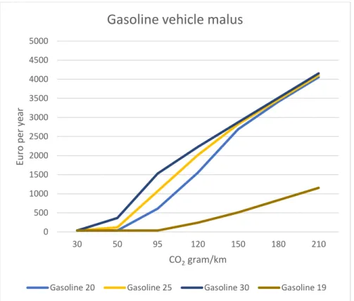
The intensified bonus-malus scenario is dynamic and its assumptions are as follows. All new cars are charged a base tax of EUR 36. In the intensified bonus-malus system, the limits for bonuses and maluses are successively lowered and the maluses successively increased. In 2030 a new car emitting less than 30 grams of CO2 per kilometer can receive a bonus. If it emits no CO2, the bonus is still EUR 6000. The bonus decreases by EUR 41.6 per each further gram of CO2 emission per kilometer. In 2030 the malus, i.e. the tax, is charged above 30 grams of CO2 emission per kilometer. In the 30–75-gram interval, the malus is EUR 16.4 per gram of CO2 emission for gasoline per year the three first years after the car is purchased. Above 75 grams, the malus is EUR 21.4 for each extra gram of CO2 emission per kilometer. Diesel cars are charged a further EUR 1.35 per gram of CO2 and an environmental charge of EUR 25 per vehicle.
The effects can be illustrated in some graphs. Fig. 1 shows the malus for gasoline cars for the current situation (Gasoline 19) and for the intensified stages of 2020, 2025, and 2030; Fig. 2 shows the same for diesel cars. As is obvious from the figures, the intensified malus becomes quite large for big emitters. One should keep in mind that the maluses will to some extent be offset by the increase in fuel efficiency that is assumed to occur over time.
14
Fig. 1. Gasoline vehicle malus, Euro per year the three first years depending on CO2 emission.
Fig. 2. Diesel vehicle malus, Euro per year the three first years depending on CO2 emission.
0 500 1000 1500 2000 2500 3000 3500 4000 4500 5000 30 50 95 120 150 180 210 Eu ro p er ye ar CO2gram/km
Gasoline vehicle malus
Gasoline 20 Gasoline 25 Gasoline 30 Gasoline 19
0 500 1000 1500 2000 2500 3000 3500 4000 4500 5000 30 50 95 120 150 180 210 Eu ro p er ye ar CO2gram/km
Diesel vehicle malus
15
3.4 A mandated biofuel blend scenario
We initially intended to calculate the effects of an intensified biofuel blending mandate. When we realized the huge uncertainties concerning price forecasts for biofuels and what a reasonable policy scenario (and therefore loss of tax revenue) could be, given these uncertainties, we decided not to incorporate assumptions of a stronger mandated biofuel blending into the estimation of the CO2 emission decrease by 2030 based on the car fleet of the other two scenarios.
This scenario has been the hardest to construct. On one hand, there is currently a strong desire to use biofuel blending to reduce CO2 emissions, manifested in high current biofuel shares and visions of continued increases in these shares. On the other hand, international trade in biofuels such as HVO has led to accelerated deforestation to grow oil palms. The latter argument has led politicians to question the ambition to increase biofuel imports from certain sources, and the EU has imposed limits on the import of such biofuels. A further implication is that this uncertainty concerning the levels of mandate and imports makes it very difficult to forecast biofuel prices.
So far, policy has proceeded on the assumption that biofuels were exempted from CO2 taxation. Current proposals from the EU commission ( https://www.svt.se/nyheter/inrikes/biodrivmedel-kan-bli-av-med-skattebefrielsen) indicate that these exemptions will be abolished. If this happens then biofuels are to be subject to CO2 taxes.
We have therefore opted for a very simplified scenario. We do not assume that the biofuel blending share will change from the levels to be enacted starting in 2020 (requiring sellers to reduce CO2 emissions from gasoline by 4.2% and from diesel by 21%). We assume that these blending
requirements can and will be met at the same fuel prices as in the reference scenario. Instead, we assume that the increasing costs will be carried as lower tax revenues, not affecting consumer welfare in the fuel market. We assume that the production costs will be unaffected by the blending mandate and that the cost of biofuels will grow by the same rate until 2030.
To illustrate the magnitude of the costs of increasing the biofuel content of fuels, we calculated the increase in the cost of replacing one liter of fossil fuel with one liter of biofuel at prices current as of October 2019.
Table 1
Production cost increase for replacing one liter of fossil fuel with one liter of biofuel and the current total tax for fossil fuel.
Production cost increase for a one-liter swap
Current price The current total tax Gasoline EUR 0.59 EUR 1.58 EUR 1.07
Diesel EUR 0.62 EUR 1.56 EUR 0.94
16
Table 1 shows the costs of increasing the share of biofuels. Replacing a liter of gasoline with ethanol will reduce CO2 emissions by 2.36 kg per liter at a cost of EUR 0.25 per kilogram of CO2. The
corresponding cost for reducing CO2 emissions by substituting HVO for diesel is EUR 0.24 per kilogram of CO2. This would be affordable if the supply of biofuels were abundant.
4. Results
In this section we present descriptive statistics for 2016, the effects on the car fleet in the reference scenario for 2030 compared with the actual car fleet in 2016 and in the policy scenarios, and distributional effects on the consumer side of the market from the 2030 scenarios. All effects on weight and energy type are presented in the shares of each vehicle type in 2030. Note that we also compare the results with the actual car fleet in 2016 to see the effect of the current policy. The results for the fuel tax scenario in 2030 are also compared with the short-term results for 2011 in Eliasson et al. (2018).
4.1 Descriptive statistics
The data on all individual adults and privately owned cars in 2016 are summarized with their means and standard deviations (not, however, for dummy variables as the standard deviations are then a function of the mean only) in Table 2. The descriptive statistics are classified into the three
geographical residence areas, i.e. large cities, small cities, and rural areas. Note also that the upper part of the table presents data on people, while the lower part presents data on cars.
17
Table 2
Descriptive statistics for the individual and car data, 2016.
Variable All Large cities Small cities Rural areas
Person data
Car owners (at least one car) 44.69% 36.69% 48.86% 58.68%
Owns one car 34.92% 30.50% 38.30% 41.19%
Owns two cars 7.26% 4.89% 7.96% 12.10%
Owns three cars 1.63% 0.90% 1.74% 3.27%
Owns four cars 0.89% 0.40% 0.86% 2.12%
Vehicle kilometers per year 6855 (10,702) 5290 (9505) 7149 (9505) 10,263 (12,710)
Disposable income, SEK per year 259,974 (952,159) 280,439 (1,251,846) 232,958 (541,611) 242,585 (447,250) Age, years 48.7 (19.5) 46.9 (19.1) 50.2 (20.1) 51.8 (19.0) Percentage employed 60.17% 61.51% 56.63% 60.96%
Distance to work in kilometers (given employment) 21.6 (65.3) 19.7 (63.9) 21.5 (68.2) 26.1 (63.5)
Has company car 3.54% 4.15% 2.53% 3.19%
No. of observations 7,758,289 3,835,120 2,136,363 1,529,734 Car data
Vehicle kilometers per year 12,218 (8220) 11,864 (8031) 11,700 (7930) 13,155 (8652)
Share of weight class, lightest 31.2% 33.6% 31.8% 27.6%
Share of weight class, medium 33.7% 32.9% 34.2% 34.3%
Share of weight class, heaviest 35.1% 33.6% 34.1% 38.1%
Age, years 10.8 (8.8) 9.7 (7.8) 11.1 (8.9) 12.0 (9.8)
Fuel consumption, liter per 10 km 0.760 (0.197) 0.760 (0.198) 0.759 (0.194) 0.761 (0.200)
Share of gasoline cars 65.94% 66.41% 67.53% 64.29%
Share of diesel cars 27.58% 25.77% 26.34% 30.67%
Share of ethanol cars 4.86% 5.37% 5.05% 4.01%
Share of electric cars 0.06% 0.07% 0.03% 0.08%
Share of all hybrid cars 0.99% 1.54% 0.66% 0.57%
No. of observations 4,358,429 1,681,648 1,309,884 1,216,948
We can see from the descriptive statistics that there are substantial differences across the geographical residence areas. The share of car owners is the largest in rural areas and smallest in large cities. The same pattern holds for those individuals who own more than one car. Furthermore, this pattern implies that total vehicle kilometers per individual are highest in rural areas and lowest in large cities. This relatively large difference is almost exclusively a result of different car-owning shares, as we can see that the vehicle kilometers per car are not that different across the
18
cities; so too is the employment status, while the distance to work, as expected, is the longest in rural areas.
In addition, car-level data show that the cars are heaviest in rural areas. Also, rural areas have the oldest cars and the highest share of diesel cars. The fuel consumption is strikingly similar across the geographical residence areas. Here, different forces move in opposite directions: more diesel cars in rural areas leads to lower fuel consumption, but this effect is offset by the heavier as well as older cars in rural areas.
4.2 Effects on car weights, driving distance, and emissions
4.2.1 Change in car weight and energy type
The following effects on the weight distribution of the car fleet are estimated using only the car fleet model.
Table 3
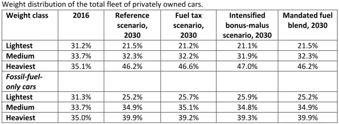
Weight distribution of the total fleet of privately owned cars.
Weight class 2016 Reference scenario, 2030 Fuel tax scenario, 2030 Intensified bonus-malus scenario, 2030 Mandated fuel blend, 2030 Lightest 31.2% 21.5% 21.2% 21.1% 21.5% Medium 33.7% 32.3% 32.2% 31.9% 32.3% Heaviest 35.1% 46.2% 46.6% 47.0% 46.2% Fossil-fuel-only cars Lightest 31.3% 25.2% 25.7% 25.9% 25.2% Medium 33.7% 34.9% 35.1% 34.8% 34.9% Heaviest 35.0% 39.9% 39.2% 39.3% 39.9%
Table 3 presents the development of the relative frequencies of three car weight classes. Note that in the mandated biofuel blend scenario in which the prices of fuel and electricity do not develop
differently from those in the reference scenario, the development of the car fleet will be the same as in the reference scenario. An important observation here is that the intensified bonus-malus scenario does not reduce the tendency toward heavier cars. On the contrary, it appears to slightly increase this tendency. This in itself increases energy consumption.
There are two main reasons for this increase in weight. The first is that for equally sized cars, an electric or a plug-in version is heavier. The second is the preference for larger cars, which is easier to satisfy when income increases. Table 3 also shows that the tendency toward heavier cars from 2016 to 2030 also holds for fossil-fuel-only cars, although this increase is lower than the increase in the entire car fleet.
19
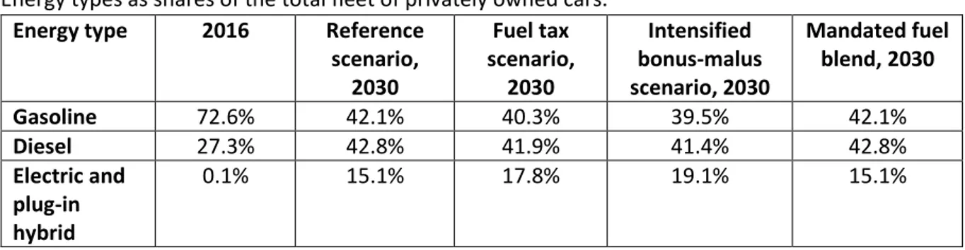
Table 4 presents the development of cars in different energy source classes. The ensuing effects on the distribution of the energy types in the car fleet are also estimated using only the car fleet model.
Table 4
Energy types as shares of the total fleet of privately owned cars.
Energy type 2016 Reference scenario, 2030 Fuel tax scenario, 2030 Intensified bonus-malus scenario, 2030 Mandated fuel blend, 2030 Gasoline 72.6% 42.1% 40.3% 39.5% 42.1% Diesel 27.3% 42.8% 41.9% 41.4% 42.8% Electric and plug-in hybrid 0.1% 15.1% 17.8% 19.1% 15.1%
The speed of introduction of electric and hybrid cars is similar in magnitude in the fuel tax and bonus-malus scenarios. As several predictions state that electric cars and plug-in hybrid cars will dominate fossil-fuel cars from a lifecycle-cost perspective, the introduction of those cars may be considered slow. There are, however, reasons why the benefits of a fossil-fuel car could exceed those of an electric car. Among those reasons are relatively quick refueling, nonexistent home charging infrastructure in apartment buildings, and difficulties driving with a trailer. In the mandated fuel bland scenario in which fuel or electricity prices do not develop differently from in the reference scenario, the development of the car fleet will be the same as in the reference scenario.
4.2.2 Reduction of CO2 emissions
In Table 5 the effects on the CO2 emissions in the scenarios are derived using the car fleet model, the car allocations to the population groups, and the elasticities of car use in the respective groups.
Table 5
Reduction of CO2 emissions in the scenarios.
Time period Reference scenario, 2030 Fuel tax scenario, 2030 Intensified bonus-malus scenario, 2030 Mandated fuel blend, 2030 2010–2016 16.0% 16.0% 16.0% 16.0% 2016–2030 24.2% 51.9% 28.0% 24.2% 2030–2030 (scenario difference) - 36.4% 5.0% 0 2010–2030 36.4% 59.6% 39.5% 36.4%
The reduction of CO2 emissions in the intensified bonus-malus scenario compared with the reference scenario is relatively small at around 5%. In the fuel tax scenario, on the other hand, the reduction is about 36%. This difference depends on the behavioral response in kilometers driven with respect to
20
the price change of fuel in the fuel tax scenario. The intensified bonus-malus scenario has no fuel-price changes compared with the reference scenario and thus no decrease in car driving.
The reduction of CO2 emissions from 2016 to 2030 in the reference scenario is estimated to be 24.2%, while the reduction in the entire Swedish transport sector between 2010 and 2016 was 16.0% (Swedish Environmental Protection Agency, 2019). We have only calculated the aggregate reduction of CO2 emissions from 2016 to 2030 in the reference scenario (24.2%). However, we have not explicitly analyzed the separate component effects of changes in income growth, energy prices, efficiency of new fossil-fuel cars, and replacement of fossil-fuel cars with electric cars due to energy-price changes, car energy-prices, and the bonus-malus system. However, we can say something about these separate effects. First, fuel-price increases alone lead to a car-driving effect that is almost exactly offset by income growth. In addition, the share of electric cars is estimated to increase from 0.1% to 15% from 2016 to 2030. This contributes to a 12% reduction of CO2 emissions if we consider that some of these electric cars are plug-in hybrids that are partly powered by fossil fuels. The increased efficiency of fossil-fuel cars in the simulated car fleet during this period is predicted to be about 17%, but note that this efficiency gain also implies a rebound effect of more driving as the price of driving decreases.
The total reduction of CO2 emissions from 2010 to 2030 in the fuel tax scenario is about 60%, while the reduction is about 40% in the intensified bonus-malus scenario. The goal for the total domestic transport sector (excluding air transport) is to reduce CO2 emissions by 70% from 2010 to 2030, implying that the private car segment in Sweden is far from the goal in the intensified bonus-malus scenario taken in isolation but comes relatively close to the goal in the fuel tax scenario.
Note that benefit cars (used partly for private trips; see discussion in section 2.2) and cars owned and used by organizations are not included in the analysis. If such cars, on average, emit less CO2 than do the cars in the overall fleet, the reduction might be larger than shown in Table 5. On the other hand, these cars are not included in any of the analyzed car fleets, i.e. the 2016 data, reference scenario, and policy scenarios in 2030. Such cars might be, in relative terms, similar to the cars in the analyzed fleets in all of the scenarios.
Note that we have not modeled any population growth during the 2016–2030 period. Incorporating such effects may counteract part of the CO2-emission reductions estimated in the analysis. If we would underestimate the CO2 reduction by not including benefit cars, this underestimation might be offset by the population increase.
21 4.2.3 Change in average vehicle kilometers
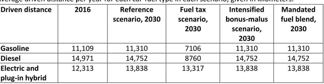
Table 6 presents the average vehicle kilometers per car for different energy types and scenarios. Here we can see that the behavioral effects are small in the reference and the intensified bonus-malus scenarios. Regarding the fuel tax scenario, on the other hand, the decrease for fossil-fueled cars is substantial. Note that there is also a small decrease in the electric and plug-in hybrid category in the fuel tax scenario compared with the reference scenario, because plug-in hybrids partly use fossil fuel.
Table 6
Average driven distance per year for each car-fuel type in each scenario, given in kilometers.
Driven distance 2016 Reference scenario, 2030 Fuel tax scenario, 2030 Intensified bonus-malus scenario, 2030 Mandated fuel blend, 2030 Gasoline 11,109 11,310 7106 11,310 11,310 Diesel 14,971 14,752 8760 14,752 14,752 Electric and plug-in hybrid 12,313 13,838 13,317 13,838 13,838
4.3 Estimates of welfare distributional effects
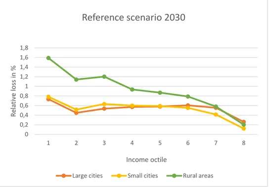
The following calculations of consumer surplus losses relative to disposable income are given for each population group. First, we present a comparison of the reference scenario of 2030 with the state as of 2016, then a comparison of distributional effects across the two car tax policies compared with the reference scenario. In all comparisons for all income groups and geographical residence areas, we present the difference between the average welfare cost per individual in a policy scenario and the average welfare cost in the reference scenario given in percent of disposal income per individual. Note that the y-axis scale is not the same in all the figures.
In Fig. 3, we can see the distributional effects for the reference scenario of 2030 compared with 2016. The effects therefore reflect current policy, including a yearly tax increase on fuel and the implemented bonus-malus system. Note that these estimated distributional effects hinge on further assumptions that are not needed when we make comparisons across the 2030 scenarios. First, we have no access to car prices for the 2016 car fleet. As the price changes for new fossil-fueled cars between 2016 and 2030 are assumed to be relatively small, we use the price of the oldest cars in 2030 as the price for all age classes in 2016. The procedure for electric and plug-in hybrid cars in 2016 is the same, but this will not be important for the analysis as the share of these cars is only 0.1% of the fleet in 2016. In addition, we have no access to the fixed circulation tax in our 2016 car data. Here we simply assume the same tax as in the reference scenario of 2030.
22
Fig. 3. Loss of consumer surplus, given in percent of disposable income.
The Fig. 3 results could be summarized in two statements: the loss in consumer surplus decreases with income, and the loss in consumer surplus is higher for rural than urban residents, especially in the lower part of the income distribution. These results indicate that the adjustment to a less fossil-fuel-dependent car fleet is easier for high-income earners than for low-income earners, and, except for the two highest income groups, easier for residents of cities than rural areas. The differences across the population groups are relatively large, showing that the 15% share of plug-in cars in 2030 is distributed mainly among the highest income octiles. The burden of the path toward a less CO2 emitting car fleet is thus carried mainly by low-income earners, especially in rural areas.
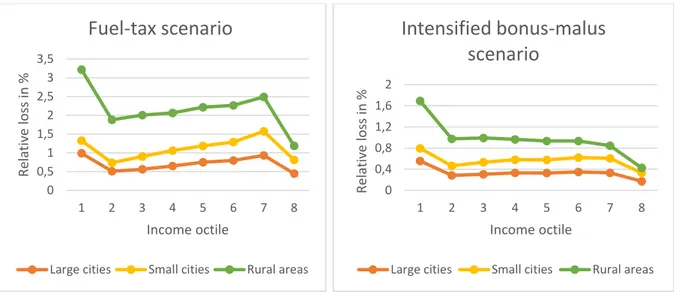
In Fig. 4, the welfare losses of the two tax policies are compared with those of the reference
scenario. The consumer welfare losses in the fuel tax scenario are generally higher than those in the intensified bonus-malus scenario. Still, we also need to consider the larger decrease in CO2 emissions in the fuel tax scenario (see Table 5). If we calculate the total consumer welfare loss in each scenario and divide this by the reduction of CO2 emissions, the result per kg of CO2 is about EUR 0.90 for the fuel tax scenario and about EUR 2.80 for the intensified bonus-malus scenario. This indicates that the welfare loss for consumers per unit decrease in CO2 emission is larger in the intensified bonus-malus system. 0 0,2 0,4 0,6 0,8 1 1,2 1,4 1,6 1,8 1 2 3 4 5 6 7 8 Re lat iv e los s in % Income octile
Reference scenario 2030
23
Fig. 4. Loss of consumer surplus, given in percent of disposable income.
We can also observe several important findings from the pattern of the figures, which largely parallel the short-term results of car-tax policies examined by Eliasson et al. (2018):
- The welfare loss is highest for people living in rural areas, followed by people living in small cities. Inhabitants in large cities suffer the lowest welfare loss.
- In most of the geographical areas in both scenarios, the policies are progressive in the octile 2–7 income interval. The exception is rural areas in the intensified bonus-malus scenario, in which the relative welfare costs decrease slightly with income. In general, the fuel tax scenario seems to be less regressive. See more about this in the discussion of the Suits index (Suits, 1977) below.
- The results for income octile 1 should be interpreted with caution. The disposable incomes of these individuals frequently lie well below a subsistence level of consumption, for example, possibly because they are young adults living with their parents or because they do not declare their full income to the tax authorities.
- Income octile 8 in all cases has the lowest relative welfare loss (except for small cities in the fuel tax scenario, in which octile 2 has a slightly lower welfare loss). Also, this result is similar to that of Eliasson et al. (2018), but the effect in the present long-term analysis is larger. The interpretation is that when car type and car use change over time, high-income individuals will adapt more easily as they can afford to pay for a car that costs more to buy but costs less to drive. Besides that, they may also benefit from the subsidies of such cars in a bonus-malus system.
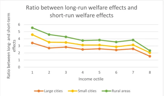
To this end, Fig. 5 presents a comparison of the distributional effects of the fuel price scenario of this study and of the 10% fuel tax increase of Eliasson et al. (2018). This is done by calculating the welfare loss ratios. Here we can see that the ratio clearly tends to decrease both with income and with how urban the geographical residence area is. Thus, in the long term, individuals with higher incomes and inhabitants in urban areas appear to have more opportunities to adapt and avoid welfare costs.
0 0,5 1 1,5 2 2,5 3 3,5 1 2 3 4 5 6 7 8 Re lat iv e los s in % Income octile
Fuel-tax scenario
Large cities Small cities Rural areas
0 0,4 0,8 1,2 1,6 2 1 2 3 4 5 6 7 8 Re lat iv e los s in % Income octile
Intensified bonus-malus
scenario
24
Fig. 5. Comparison of long- and short-term distributional effects.
In addition, we measure the progressivity of the policies using the Suits index (Suits, 1977). A flat-rate policy has a Suits index value of 0, a regressive policy has a negative Suits index, and a progressive policy a positive index; the index ranges between –1 and 1. Table 7 shows the results of two Suits index calculations for two octile selections from the population. We have excluded income octile 1 and present the index both including and excluding income octile 8. In general, the policies are regressive when income octile 8 is included, but most of them are progressive in the octile 2–7 interval. In addition, the intensified bonus-malus scenario is clearly more regressive than the fuel tax scenario. In fact, the intensified bonus-malus scenario is regressive in rural areas even in the octile 2– 7 interval.
Table 7
Suits index for both policies and all geographical areas.
Fuel tax scenario, 2030 Intensified bonus-malus scenario, 2030 Large cities Small
cities
Rural areas
Large cities Small cities Rural areas Income
octiles 2–8 –0.056 –0.019 –0.096 –0.117 –0.090 –0.161 Income
octiles 2–7 0.105 0.121 0.049 0.023 0.036 –0.029
Compared with the short-term analysis of the distributional effects of a 10% fuel tax increase by Eliasson et al. (2018), our analysis shows a more regressive outcome of the policies. This follows from the fact that subsidies of new cars (the bonus in the bonus-malus system) and adaptation to higher gasoline and diesel prices by buying a more efficient and/or electric car are both more accessible for individuals with high disposable income.
0 1 2 3 4 5 6 1 2 3 4 5 6 7 8 Rat io b etwe en lon g-an d s h o rt -term ef fe cts Income octile
Ratio between long-run welfare effects and
short-run welfare effects
25
As noted above, employer-provided benefit cars that are partly used for private trips are not included in the analysis. This type of benefit is highly skewed toward the highest income octiles, as the tax deduction depends on the marginal rate of income tax, which is higher for higher incomes. As a relatively simple calculation example of how large this effect might be, we start by noting that about 5% of individuals in the 7th octile and about 20% in the 8th octile have access to a benefit car. Assuming that 60% of these cars (which are nearly always under three years old) are fossil-fuel cars and that these are driven relatively long distances, the increased relative welfare loss in the fuel tax scenario for the highest income octile is calculated to change by 0.08–0.21 percentage points (depending on the geographical residence area). In the 7th octile, the effect is a lower increase by 0.02–0.05 percentage points. In reality, these effects are likely to be lower, as these company cars will even more likely be electric cars and plug-in hybrid cars than will privately owned cars. In the intensified bonus-malus system, the effect is assumed to be even lower, as most of these cars are expected to be cars receiving bonuses. The effect of not including company cars used for private trips in our analysis is therefore assessed to be small.
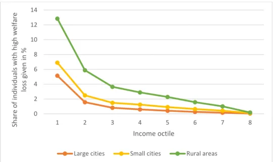
Moving away from average analysis only, we calculate the share of each population group that has a welfare loss exceeding 8% of disposable income in the fuel tax scenario. Here again we use the group-specific average fuel consumption and elasticity of driving distance with respect to fuel price. The fuel price used is a weighted average of the gasoline price and diesel price with respect to the distribution of gasoline and diesel cars in the total car fleet in this policy scenario. To find differences at the population-group level, we use the population group driving distance in 2016 to estimate the driving distance in the fuel tax scenario of 2030. Note also that we do not include fixed car costs, as we do not have an individual car choice sub-model.
The result of this analysis is presented in Fig. 6. We can see that the share of the population group with large relative welfare losses is higher the lower the income is. Furthermore, the share decreases rapidly with income and approaches zero in income octile 6 in urban areas and in the highest income octile in rural areas. In addition, the share is the largest in rural rather than urban areas, where the difference between small and large cities is relatively small.
26
Fig. 6. Share in percent of individuals with a relative welfare loss exceeding 8% in the fuel tax
scenario.
4.4 Sensitivity analyses
4.4.1 Sensitivity analysis with respect to depreciation rate
We have assumed a fixed yearly depreciation rate of 15% of current value for cars. Here, this assumption is changed both to a lower depreciation rate of 10% and a higher depreciation rate of 20%. The assumed changes in depreciation rate lead to very small changes in the estimated welfare losses, and even more importantly, the pattern in the figures is almost completely the same (figures not shown). The latter suggests that the assumed (constant) depreciation rate is relatively
unimportant for the outcome of the analysis. However, if we had been able to model different depreciation rates for different car types and/or policy scenarios, this might have influenced the results of our analysis (cf. Jacobsen and Benthem, 2015; Bento et al., 2018a).
4.4.2 Sensitivity analysis with respect to elasticity of demand for driving distance
When the assumed elasticity of car use with respect to fuel price is lower, namely, in the range of –0.01 to –0.10 (see Table A3 in the Appendix), we can see in Fig. 7 that the intensified bonus-malus scenario remains more or less unchanged, which is completely as expected. In the fuel tax scenario, this lower elasticity assumption seems to make the policy slightly more regressive, especially in the rural areas. This is also confirmed by the Suits index (not shown). Furthermore, the consumer welfare losses increase substantially when we assume a smaller reduction in car use when fossil fuel prices increase. 0 2 4 6 8 10 12 14 1 2 3 4 5 6 7 8 Sh ar e o f in d iv id u als with h igh w elf ar e los s giv en in % Income octile
27
Fig. 7. Distributional effects with the assumption of lower elasticity of car use with respect to fuel
price.
However, the most important result from assuming a smaller behavioral response to fuel-price increases is that the reduction of CO2 emissions will be dramatically lower than shown in Table 4. Here, the CO2 emissions are estimated to be reduced by only 6.6% in the scenario with increased fuel prices. This highlights the importance of the assumed behavioral response in terms of car use to policies for reaching ambitious CO2-emission goals. Finally, note also that the predicted reduction of CO2 emissions between 2016 and 2030 in the reference scenario is strongly dependent on behavioral changes, as the real prices of gasoline and diesel also increase during this period. The decrease in CO2 emissions with the assumption of low elasticity is only about 11% compared with 24% with the baseline-assumption elasticities. With the assumption of lower elasticity of car driving with respect to fuel price, the reduction of CO2 emissions in the fuel tax scenario is estimated to be about 30% from 2010 to 2030 instead of about 60% with the baseline assumption of elasticities.
5. Discussion
This analysis has both important strengths and some important limitations. One important strength is that the analysis is based on models of actual choices of car attributes, allowing for a model-based representation of future car-type choices. The analysis also uses detailed data on incomes,
geographical residence areas, car ownership, and car use for all adult Swedes in 2016. This allows for a highly differentiated and geographically resolved representation of effects. In the analysis, we abstract from the development of the population, residence, individual car ownership, and differentiated income growth. This can be justified, as we can distinguish how individuals with different income levels, residential area types, and car use patterns are affected by the policy instruments.
There are four important limitations of the analysis. First, the car choice and use of cars owned by companies and organizations are not considered in the analysis. Second, the car supply is not
0 1 2 3 4 5 1 2 3 4 5 6 7 8 Re lat iv e los s in % Income octile
Fuel tax scenario
Large cities Small cities Rural areas
0 0,4 0,8 1,2 1,6 2 1 2 3 4 5 6 7 8 Re lat iv e los s in % Income octile