Predicting dynamic fuel oil consumption on ships with automated machine learning

(1)

http://www.diva-portal.org

Postprint

This is the accepted version of a paper presented at 10th International Conference on

Applied Energy (ICAE2018), Hong Kong, China, August 22-25, 2018.

Citation for the original published paper:

Ahlgren, F., Mondejar, M E., Thern, M. (2019)

Predicting dynamic fuel oil consumption on ships with automated machine learning In: Prof. J.Yanab, Prof. H.Yang, cDr. H.Lid, Dr. X.Chene (ed.), Innovative Solutions

for Energy Transitions: Proceedings of the 10th International Conference on Applied Energy (ICAE2018) (pp. 6126-6131). Elsevier

Energy Procedia

https://doi.org/10.1016/j.egypro.2019.01.499

N.B. When citing this work, cite the original published paper.

Permanent link to this version:

(2)

ScienceDirect

Energy Procedia 00 (2018) 000–000

www.elsevier.com/locate/procedia

Selection and peer-review under responsibility of the scientific committee of the 10th_{International Conference on Applied Energy (ICAE2018).}

10

th

_{International Conference on Applied Energy (ICAE2018), 22-25 August 2018, Hong Kong,}

China

Predicting Dynamic Fuel Oil Consumption on Ships with

Automated Machine Learning

Fredrik Ahlgren

a*

_{, Maria E. Mondejar}

b

_{, Marcus Thern}

c a_{Linnaeus University, Kalmar 39354, Sweden}

b_{Technical University of Denmark, Kgs. Lyngby 2800, Denmark} c_{Lund University, Lund 22100, Sweden}

Abstract

This study demonstrates a method for predicting the dynamic fuel consumption on board ships using automated machine learning algorithms, fed only with data for larger time intervals from 12 hours up to 96 hours. The machine learning algorithm trained on dynamic data from shorter time intervals of the engine features together with longer time interval data for the fuel consumption. To give the operator and ship owner real-time energy efficiency statistics, it is essential to be able to predict the dynamic fuel oil consumption. The conventional approach to getting these data is by installing additional mass flow meters, but these come with added cost and complexity. In this study, we propose a machine learning approach using auto machine learning optimisation, with already available data from the machinery logging system.

Selection and peer-review under responsibility of the scientific committee of the 10th_{International Conference on Applied}

Energy (ICAE2018).

Keywords: shipping; auto machine learning; energy efficiency; predicting fuel consumption

1. Introduction

The shipping sector is a significant contributor to global carbon emissions, and in 2014 the sector contributed to about 2.9 % of the world's total greenhouse gas emissions and is expected to take even a greater share in the future [1]. The shipping sector needs to reduce the emissions, and energy efficiency is one important method to mitigate

*_{Corresponding author. Tel.: +46-480-497671; fax: +46-480-497650.}

(3)

2 F. Ahlgren, M. E. Mondejar, M. Thern / Energy Procedia 00 (2018) 000–000

and reduce carbon emissions from the shipping sector [2]. Operational efficiency is a very significant factor, as knowing the effects of the waves, wind, rudder position, speed and trim in real time by measuring the current energy consumption is essential to get the right decision tools for the crew. To set the ship speed, trim and bearing at an optimum condition measurement of the current fuel consumption are needed. This is essential as a base for an optimisation tool as well as manual decision making and adjustments for the crew during operation. The fuel consumption is often not measured and presented in real time, and many old ships in operation still rely on tank meters and daily measuring. A mass flow meter is often installed to present data of the instantaneous fuel consumption, but this comes with both an added cost and system complexity. The additional cost of a mass flow meter is in the range of 3000-19,000 USD, excluding of installation costs [3]. The combination of mass flow meters and machine learning (ML) algorithms that are coupled with already available data creates the opportunity to predict individual consumers without the need to install a flow meter on each point. In ships not equipped with fuel flow meters, there is always a noon-report where the tank-meters are logged each day. By using this noon-report in combination with already available engine data, an ML algorithm can predict the fuel consumption even for shorter time intervals which give the operator a better understanding on how the ships' energy consumption.

The data used in this study is from a cruise ship built in 2004, travelling between Stockholm and Mariehamn in the Baltic Sea. It is a medium-sized cruise ship, 180 m long, with a total of eight engines. Four main engines used for propulsion which is connected to two propellers, and four auxiliary generators which produce electricity. The engines are divided into two fuel lines, starboard and port, called fuel line 0 and 1 in this article. There is both a set of older initially installed volume flow meters which are used as the model target in this study and newer mass flow meters which are not connected to a logging system.

Studies on predicting fuel consumption on ships have been done before. Wang et al. proposed a least absolute shrinkage and selector operator (LASSO) regression predicting the fuel consumption for 97 container ships, with features on ship and weather data extracted from a fleet management system [4]. The LASSO regression produced better results compared to support vector machines (SVR), artificial neural networks (ANN) and Gaussian process regression (GP). Meng et al. used operational data, based on 24 h daily snapshots, from two sister container ships and using regression modelling predicting the daily fuel consumption [5]. Bal et al. demonstrated an ANN with training data based on noon-reports from an oil tanker, which was used as an input a forecasting model to a decision support system [6]. The algorithm could predict the fuel consumption in mton/h using training features from both the engines rpm, ship speed, weather data etc. So far, no studies have been done on using state-of-the-art auto-ML tools, predicting the instant fuel consumption for ships using noon-report data.

In this study, we propose a machine learning approach by training an ML algorithm with dynamic data from the ships' logging system and using high time intervals for fuel sums, 12 h up to 96 h. The aggregated fuel sums used in this study are from already installed fuel meters, but in a different scenario, this could be either manual or automatic tank measurements as well as data from bunkering reports, this means that the operator can get real-time fuel consumption even though it is not actually measured more than for longer and sparse time intervals. This study demonstrates a method which could increase the accuracy of existing decision tool systems at both a reduced cost and complexity.

2. Method

Machine learning is the field within computer science that uses statistical algorithms to learn on data (or experience) and from that make predictions without being explicit programmed [7]. There is a vast amount of different ML algorithms, each of them with their specific strengths and weaknesses. A more complex algorithm can be prone to overfitting, or the complexity can make the algorithm take longer to train and execute without being able to make better predictions. One of the simplest forms of ML-algorithm is the linear regression, where a linear correlation is fitted with the least square method. However, a linear correlation is a simplification of reality, and more complex models are needed to get a better fit for real applications. With an added complexity comes an added cost of computing time as every model contains a various amount of hyperparameters which needs to be tuned for optimal

(4)

fit [8]. When training an ML-model the inputs, which can be sensor data, are called features, and the predicted value and model output is called the label.

The classical approach in ML is supervised learning, which requires a certain amount of experience to choose the right model, pre-processors and optimising hyperparameters. In this study, we utilise an auto machine learning framework for optimising and choosing a model, which means that algorithms are used for the part that generally is very dependent on the experience of the ML-practitioner. Auto Machine Learning (AutoML) is the concept of automating the work of the data scientist, running optimisation routines on choosing both the best pre-processing of data, algorithm, and tuning of hyper-parameters. All this is put together in a pipeline, which is a Python object containing several ML-classes, where often a pre-processor and one or several ML-models are trained in series. The advantage of using pipelines of models it that several simple models can together perform very well if integrated in series. To get a robust algorithm and a good prediction the data needs to be pre-processed, the right algorithm chosen and the data needs to be divided in a random train and test set. Depending on how large quantities of data available the train and test split it somewhere between 50-90 % (larger for big data sets) [8]. All models need some form of parameter input which is defined as hyperparameters. Hyperparameters for an ML-model can, for instance, be the number of layers in a neural network, loss factor for training or number of clusters in a K-means [8].

The data was extracted from the ships' machinery logging system using a database exporter tool. The exported data was exported in several overlapping Microsoft Excel 2007 files, and all data was consolidated into one database and stored in a hierarchical data format (HDF-database) using the Python Pandas library [9]. In this study, there is a total of 30624 sample data points, in the period between 2014-02-01 to 2014-12-01. The period is chosen because of inconsistent data at the end of the period, due to the ship is shifting to marine diesel fuel before the sulphur emission control area was enforced in 2015-01-01 [10]. All data are initially logged in the ship database in 1-minute intervals and is averaged to a 15-min interval when exported. The training data for the different training setups were created for each model training by resampling the time series database by the average. Test number 0 and 1 correspond to each fuel line, starboard and port side. The models are trained in a total of four time-intervals, 12 h, 24 h, 48 h and 96 h. The time intervals were chosen due to test how large interval could be used and still get a decent prediction. A larger interval than 96 h was not possible using this dataset as it would have been a too small training sample (less than 70 training samples), and four days is still a significantly longer time span than the regular noon report which is done each day.

The model was trained using the labels, engine fuel rack position (FRP), engine RPM, turbo RPM and turbo exhaust temperature. In total there are eight engines, divided into four main engines for propulsion and four auxiliary electricity generators. They are divided into two separate fuel lines, with a separate fuel meter for each fuel line. Each fuel line is representing one trained model with 64 features (FRP, engine_RPM, turbo_RPM, exhaust_T) and one label for FO-flow.

As demonstrated in Figure 1, the training is done with a random set of the data and validated using the test data. The train and test data are extracted using the scikit-learn cross validation class, and a total of 10 different train/test splits were done for the training, using a set list of random seeds which is saved for repeatability. To be able to make the model comparison between all training setups, all tests were done with the same set amount of 70 training samples and 10 test samples. This ratio (87.5 %/12.5 %) was chosen as the train/test ratio because the 96 h-interval contains only a total of 80 data points which is considered to be a small training set. Even though for instance the 12 h-interval consists of 638 samples and the model training would get significantly better results if considering a larger ratio of the input data.

In this study we use the AutoML-library Tree Pipeline Optimization Tool (TPOT) for optimising the best model selection, hyperparameters as well as pre-processing the data [11]. The TPOT-library utilises a set of regression ML-models in the extensive Python library scikit-learn [12]. In all model training using the TPOT as a model optimiser, 10 generations of a subset of models from the scikit-learn library are evaluated with a population size of 50 for each

(5)

generation. The optimisation is done by the tool by minimising the mean squared error (MSE) between the train and test data.

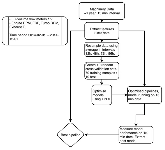
Figure 1. Flowchart of pre-processing, cross-validation, training and selecting best pipeline.

The optimised model pipeline that performed the best on the 96 h-interval data was chosen as the overall best performing pipeline, as can be seen in Figure 1. The most extended time interval was chosen as the selecting parameter because we wanted to pick the most robust model, as predicting on very sparse and high time intervals should leave less information to train the ML-model.

Machinery Data ~1 year, 15 min interval

Extract features Filter data - FO-volume ﬂow meters 1/2

- Engine RPM, FRP, Turbo RPM, Exhaust T.

Time period 02-01 -- 2014-12-01

Create 10 random cross validation sets. 70 training samples / 10 test.

Optimise models using TPOT Resample data using average in intervals 12h, 48h, 72h, 96h. Optimised pipelines, model running on 15 min data. Measure model perfomance on 15-min data. Extract best model. Best pipeline

(6)

3. Results and discussion

The best performing model pipeline on predicting the 15-min interval data was from random seed 4 and this was using the 96 h interval data as training input. The model scored an R2-score of 0.9936 on fuel line 1. The best pipeline was a standard scaler and a linear support vector regression machine, with the following hyperparameters: LinearSVR(StandardScaler(input_matrix), C=0.1, dual=True, epsilon=0.001, loss=epsilon_insensitive, tol=1e-05). The standard scaler function is scaling the model input data by subtracting the median value in the numerator and dividing with the standard deviation. A linear support vector regression is support vector regression using a linear kernel [13].

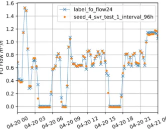
Figure 2. 96 h model prediction 15-min interval data, 1 year. Figure 3. 96 h model prediction one day operation

In Fig. 2 the best performing 96 h-model for fuel line 1 (test 1) is presented in a scatterplot for a full year of operation with the label (FO-flow) on the X-axis. The model demonstrates an R2-score of 0.993873 when predicting on the full dataset using in the 15-min interval. It can be seen that the model has very few outliers even for the full year dataset over 1.0 m3/h and makes a worse prediction during lower fuel flows. It can be argued that the explanation for this is because there is a lot of manoeuvring during low load conditions and therefore many dynamics which cannot be picked up by a 96 h-average interval.

As the normal operation for the ship is a daily route between two ports also including slow speeds in the archipelago, there are high dynamic loads (high fuel consumption) for short time intervals which will be smoothed out when averaging the engine features for 96 h. As the days' operational profile is very similar each day, a random day is presented in Fig. 3 for demonstrating model performance during both lower loads and dynamic conditions. It can be seen that the model predicts the higher high dynamic loads very well but has some deviations between the model and label during the transition between medium loads to zero loads. The ML-model for fuel line 1 (test 1) performed better than fuel line 0, and if looking at the full dataset averaging the results from both fuel lines the model performance for seed 2 scored a total R2-score of 0.9865.

(7)

4. Conclusion

We have presented a method for predicting the dynamic fuel consumption with Open Source machine learning algorithms for a ship using the total fuel sums for more extended time periods, 12 h – 96 h. This can be used as a complement to an installation of additional mass flow meters, and a better base for the decision supports systems on board. The results indicate a model which can predict dynamics of the fuel consumption despite using only sparse data for the fuel readings. This study is based on a single case and needs to be extended to have a more generalised method. The method indicates that operation data that are already available on many ships can be used in conjunction with noon-reports or seldom bunker intervals, to predict an instant fuel consumption, this without the additional cost of installation of more sensors.

5. References

[1] Smith TWP, Jalkanen JP, Anderson BA, Corbett JJ, Faber J, Hanayama S, et al. Third IMO GHG Study 2014. London: 2014.

[2] Acomi N, Acomi OC. Improving the Voyage Energy Efficiency by Using EEOI. Procedia - Soc Behav Sci 2014;138:531–6. doi:10.1016/j.sbspro.2014.07.234.

[3] Coriolis Mass Flow Meters | Instrumart 2018. https://www.instrumart.com/categories/5678/coriolis-mass-flow-meters (accessed March 14, 2018).

[4] Wang S, Ji B, Zhao J, Liu W, Xu T. Predicting ship fuel consumption based on LASSO regression. Transp Res Part Transp Environ 2017. doi:10.1016/j.trd.2017.09.014.

[5] Meng Q, Du Y, Wang Y. Shipping log data based container ship fuel efficiency modeling. Transp Res Part B Methodol 2016;83:207–29. doi:10.1016/j.trb.2015.11.007.

[6] Bal Beşikçi E, Arslan O, Turan O, Ölçer AI. An artificial neural network based decision support system for energy efficient ship operations. Comput Oper Res 2016;66:393–401. doi:10.1016/j.cor.2015.04.004. [7] Samuel AL. Some Studies in Machine Learning Using the Game of Checkers 1959:21.

[8] Raschka S. Python machine learning: unlock deeper insights into machine learning with this vital guide to cutting-edge predictive analytics. Birmingham Mumbai: Packt Publishing open source; 2016.

[9] McKinney W. Data Structures for Statistical Computing in Python. In: van der Walt S, Millman J, editors. Proc. 9th Python Sci. Conf., 2010, p. 51–6.

[10] IMO - 2010 - RESOLUTION MEPC.176(58) (Revised MARPOL Annex VI). International Maritime Organization; 2010.

[11] Olson RS, Urbanowicz RJ, Moore JH, Bartley N. Evaluation of a Tree-based Pipeline Optimization Tool for Automating Data Science. Proc. Genet. Evol. Comput. Conf. 2016, Denver, Colorado, USA: ACM; 2016, p. 485–92. doi:10.1145/2908812.2908918.

[12] Pedregosa F, Varoquaux G, Gramfort A, Michel V, Thirion B. Scikit-learn: Machine Learning in Python. J Mach Learn Res n.d.;12:6.

[13] Smola AJ, Schölkopf B. A tutorial on support vector regression. Stat Comput 2004;14:199–222. doi:10.1023/B:STCO.0000035301.49549.88.