Advanced Characterization of Exoplanet Host Stars

Juni 2020

Advanced Characterization of

Exoplanet Host Stars

Khaled Al Moulla

Masterprogrammet i fysik

Teknisk- naturvetenskaplig fakultet UTH-enheten Besöksadress: Ångströmlaboratoriet Lägerhyddsvägen 1 Hus 4, Plan 0 Postadress: Box 536 751 21 Uppsala Telefon: 018 – 471 30 03 Telefax: 018 – 471 30 00 Hemsida: http://www.teknat.uu.se/student Khaled Al Moulla

The spectroscopic determination of stellar properties is important for subsequent studies of exoplanet atmospheres. In this thesis, HARPS data for 6 exoplanet-hosting, late-type stars is processed to achieve an average signal-to-noise ratio of ~105. Together with line data, the SME tool is used to synthesize spectra and interpolate model photospheres with which chi-square minimization is performed. Fundamental parameters are derived to an overall precision of 191 K in effective temperature, 0.88 dex in surface gravity and 0.21 dex in metallicity. For 5 of the stars, the parameters are thereafter used to compute specific intensities across the stellar discs.

Primary improvements could be made in regards to the stellar models, i.a. through the update of atomic properties and inclusion of

magnetic fields. The numerical derivation can also be handled more carefully by excluding parameter-insensitive spectral regions. Keywords. stars: exoplanet hosts - fundamental parameters - spectroscopy: HARPS - SME

FYSMAS1119

Examinator: Andreas Korn

Ämnesgranskare: Bengt Edvardsson Handledare: Nikolai Piskunov

Den spektroskopiska bestämningen av stjärnegenskaper är viktig för efterföljande studier av exoplaneters atmosfärer. I denna avhan-dling bearbetas HARPS-data från 6 stjärnor av sen typ som hyser exoplaneter för att uppnå en genomsnittlig signal-till-bruskvot på

∼105. Tillsammans med linjedata, används SME-programvaran för

att syntetisera spektra och interpolera modellfotosfärer med vilka chi-kvadratminimering genomförs.

Fundamentala parametrar härleds till en medelprecision på 191 K i effektiv temperatur, 0.88 dex i ytgravitation och 0.21 dex i metallicitet. För 5 av stjärnorna används parametrarna till att därefter beräkna specifika intensiteter över stjärnornas projicerade ytor.

Huvudsakliga förbättringar kan göras med avseende på stjärnmod-ellerna, bl.a. genom uppdatering av atomära egenskaper och inklud-ering av magnetiska fält. Den numeriska härledningen kan också hanteras med högre noggrannhet genom att avsiktligt exkludera pa-rameterokänsliga spektralregioner.

Nyckelord. stjärnor: exoplanetvärdar fundamentala parametrar -spektroskopi: HARPS - SME

Under de dystra månaderna satt själen hopsjunken och livlös

men kroppen gick raka vägen till dig. Natthimlen råmade.

Vi tjuvmjölkade kosmos och överlevde.

List of Acronyms i Chapter 1: Introduction 1 1.1 Background . . . 1 1.2 Purpose . . . 1 Chapter 2: Theory 2 2.1 Stellar spectra . . . 2 2.1.1 Classification . . . 2 2.1.2 Radiative transfer . . . 3

2.1.3 Line formation and broadening . . . 4

2.2 Dependence on ... . . 6 2.2.1 ... temperature . . . 6 2.2.2 ... gravity . . . 7 2.2.3 ... metallicity . . . 8 2.3 Instrumentation . . . 9 2.3.1 Spectrographs . . . 9 2.3.2 Detectors . . . 11 2.3.3 Noise . . . 12 Chapter 3: Methods 13 3.1 Target selection . . . 13 3.2 Data processing. . . 13 3.2.1 Reduction . . . 13 3.2.2 Wavelength calibration . . . 15 3.2.3 Summation . . . 15 3.2.4 Continuum normalization . . . 17 3.2.5 SNR filtration . . . 17 3.3 Spectral synthesis . . . 19

4.2 Derived parameters . . . 23 4.3 Limb darkening . . . 23 Chapter 5: Discussion 27 5.1 Uncertainties . . . 27 5.2 Further improvements . . . 27 Chapter 6: Conclusion 29 Acknowledgements 30 Appendix A: Observations 31 Bibliography 33

ABO Anstee-Barklem-O’Mara ADC analog-to-digital converter ADU analog-to-digital unit CCD charged-coupled device EDE Exoplanet Data Explorer ESO European Southern Observatory FSR free spectral range

GUI graphical user interface

HARPS High-Accuracy Radial Velocity Planet Searcher HWHM half-width at half-maximum

LDC limb darkening coefficient LTE local thermodynamic equilibrium NIR near-infrared

NLTE non-LTE

PSF point spread function QE quantum efficiency RV radial velocity

SME Spectroscopy Made Easy SNR signal-to-noise ratio

VALD Vienna Atomic Line Database

Chapter 1

Introduction

1.1

Background

The field of exoplanet research has in recent times grown increasingly topical, with the advancement of precise radial velocity (RV) measurements now enabling the discovery of Earth-sized companions (see e.g. Mayor et al. 2008). In order to carry out in-depth studies (atmospheric composition, habitability, etc.) of these planetary systems, it is of utmost importance to have a detailed description of their stellar hosts.

Historically, fundamental stellar parameters have been determined via semi-direct methods of varying reliability (Adibekyan et al. 2018). Temperature, for example, can be obtained empirically through photometric calibrations. Surface gravity can be calculated from the stellar mass and radius; the former is either inferred from mass-luminosity relationships or requires the star to be part of a spectroscopic binary, and the latter is measured with interferometry, binary eclipses or lunar occultations. Whereas chemical composition is impossible to investigate directly.

1.2

Purpose

The approach of spectroscopy is versatile and practical for most types of characterization. The purpose of this thesis is to spectroscopically determine the fundamental parameters for a sample of stars hosting transiting exoplanets. Similar studies (e.g. Santos et al. 2004) have focused on equivalent width measurements of single lines, which heavily rely on the quality of atomic properties, and are sometimes hindered by severe line blending especially in cooler stars where molecules form absorption bands. To mitigate the impact of uncertainty, this work will perform spectral synthesis across wavelength regions containing thousands of lines. Together with stellar models, the derived parameters will be utilized to extract intensity variations along the transit paths, useful for subsequent exploration of exoatmospheric transmission spectra.

Chapter 2

Theory

2.1

Stellar spectra

2.1.1

Classification

In the optical wavelength region, many stars showcase prominent hydrogen lines from the Balmer series, i.e. electron transitions originating in energy level n = 2. The series notation consists of the letter H assigned a subscript from the Greek alphabet, e.g. the transition 2 → 3 is called Hα, 2 → 4

is called Hβ, and so on.

When astronomers first started to observe absorption lines in stellar spectra, they did not under-stand what caused them (Böhm-Vitense 1989). Still, they began classifying stars, with capital letters of the English alphabet, based on the strength of these Balmer lines in descending order. Later on, it was discovered that stellar radiation is well-described as a theoretical black body, whose spectral energy distribution is given by the Planck function,

Bλ = 2hc

2

λ5

1

ehc/λkT ₋1, (2.1)

where h and k are Planck’s and Boltzmann’s constant, respectively, c the vacuum light speed, λ the wavelength, and T the temperature. Although the temperature of a star depends on the depth, this allowed the definition an effective temperature, Teff, equivalent to the temperature of a black body which generates the same wavelength-integrated flux, according to the Stefan-Boltzmann law,

F = σT_eff4, (2.2)

where σ is Stefan-Boltzmann’s constant. With decreasing effective temperature, the stellar spectra exhibit a clear transition from hydrogen and helium lines to those of heavier elements, collectively called metals. Some of the old letters were kept, resulting in the sequence OBAFGKM, known as the Harvard system. The spectral types are further subdivided by the numbers 0–9, and followed by a Roman numeral to denote the luminosity class, such as ‘V’ for main-sequence stars.

Another misnomer which has survived is the division of early- and late-type stars. The observed range of temperatures was thought to be evolutionarily explained which is incorrect since stars do not evolve along the main sequence, however, the terms are nowadays used to reference OBA-stars as early-type and FGKM-stars as late-type.

2.1.2

Radiative transfer

Considering an intensity beam of a certain wavelength, Iλ, the various atomic processes inside a

stellar photosphere result in the following differential equation (Carroll & Ostlie 2017), dIλ = `−(lλ+ κλ)Iλ+ jλl+ j

κ

λ˘ ρdx, (2.3)

where x is the traveled distance, and ρ the density. The remaining variables represent the mass absorption coefficients (also called opacities) for lines and continuum, lλ and κλ, respectively, and

the corresponding emission coefficients, jl

λ and jλκ. Two essential quantities can be introduced. First,

the source function is simply the emission to absorption ratio,

Sλ =

j_λl + j_λκ lλ+ κλ

. (2.4)

Under the assumption that temperature variations inside the star occur at distances larger than the mean free path of photons, which is referred to as local thermodynamic equilibrium (LTE), the source function is equal to the Planck function, Sλ= Bλ. Second, the optical depth, τλ, is defined as

dτλ = −(lλ+ κλ)ρ dx, (2.5)

and can be interpreted as the multiple of mean free paths between the depth of formation and the top of the photosphere. Optical depth—opposite to the geometrical depth x—is measured radially

inward, hence the minus sign. Eq. (2.3) can then be rewritten into

dIλ

dτλ

= Iλ− Sλ, (2.6)

known as the radiative transfer equation.

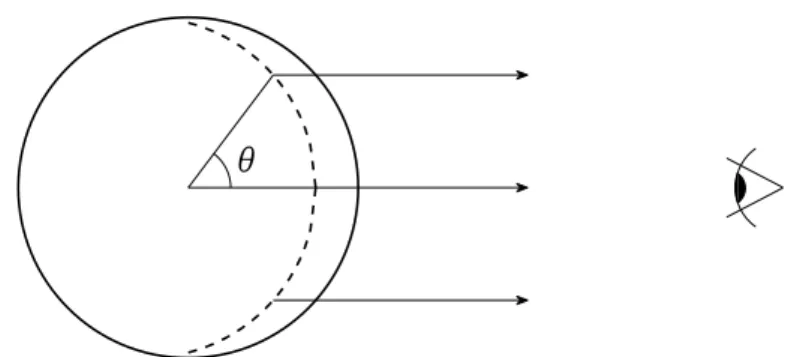
The opacity dictates how far into a star the observer sees. This entails another important aspect, namely limb darkening, which is the variation in intensity across the stellar disc. The effect is best illustrated by imagining a surface of equal vertical optical depth, i.e. along the direction to the observer, as in Fig. 2.1. The implication is that progressively shallower layers are viewed closer to the edge. As the temperature decreases upward, so does the radiation. From its geometry, the limb darkening can be assumed azimuthally independent, and the intensity is usually given as a function of µ = cos θ.

surface-θ

Figure 2.1 Illustration of limb darkening. For light emerging from a layer of equal optical depth along the

line of sight, the observer sees deepest into the star at its disc center. integrated intensity along the line of sight,

Fλ =

Z

Iλcos θ dΩ. (2.7)

Apart from recreating the flux, model photospheres have the great advantage of also providing specific intensities. In the study of exoatmospheric transmission spectra, these are needed to disentangle the stellar and planetary contributions. An exoplanet can be thought of as having a solid—or at least completely opaque—core of radius Rp with a semi-transparent atmosphere of height H on top (Aronson & Waldén 2015). During a transit, the net spectrum will be

Fλ,net= Fλ− 1 R?2 ˜ R_p2 Z Ap Iλdµ + (H2+ 2RpH) Z Aa Iλdµ ¸ , (2.8)

where R? is the stellar radius, and A_p= πR_p2 and A_a= π(R_p+ H)2− A_p are the projected areas of

the core and atmosphere, respectively.

2.1.3

Line formation and broadening

In the classical description, absorption lines are formed via the interaction between an electromagnetic wave and a bound, oscillating electron (Mihalas 1970), whose equation of motion is

me(:x + ω₀2x) = eE0eiωt−2meγ 9x, (2.9)

where e, me and x are the electron charge, mass and position, E0 the electric field strength, ω0 and ω the angular frequencies of the undamped and driven motions, and γ the damping parameter.

By equating the radiated power of the wave and electron, it can be shown that the absorption coefficient per frequency, ν, is approximately

αν ≈2 πe2 mec

γ

∆ω2_{+ γ}2, (2.10)

half-maximum (HWHM) γ. The total absorption coefficient, integrated over all frequencies, has been found to be overestimated due to quantum mechanical effects for which a dimensionless correction, 0 ≤ f ≤ 1, called the oscillator strength, is introduced,

α = Z ∞ 0 ανdν ≈ πe2 mec → fπe 2 mec . (2.11)

Apart from the natural broadening mentioned above, spectral lines are also subject to collisional and Doppler broadening. The former arises due to the interplay with certain kinds of perturbers. In the Unsöld (1955) formalism, the induced shift is described by a power law,

∆ω = Cn

rn, (2.12)

where r is the atom-perturber distance, Cn the interaction constant, and n an integer representing a

family of broadening effects:

n=     

2 linear Stark (2.13a)

4 quadratic Stark (2.13b)

6 van der Waals (2.13c)

Each n translates to its own dispersion profile. The total HWHM is then the sum of the individual contributions,

γ_tot = γ +X n

γn. (2.14)

The atom velocities, originating from a Maxwellian distribution or turbulent motion, cause a Doppler shift, ∆ωD= ω_c0 d 2kT m_a + v 2 mic, (2.15)

where T is the equilibrium temperature, ma the atom mass, and vmic the microturbulence.

The extended absorption coefficient becomes the convolution of a Lorentzian and Gaussian, known as a Voigt function, αν = 2f πe2 mec γ_tot ∆ω2_{+ γ}2 tot ∗ ? π ∆ωDe −(∆ω/∆ω_D)2_{. (2.16)}

The conversion between frequency and wavelength units is found through

ανdν = αλdλ, (2.17)

2.2

Dependence on ...

The following subsections on various dependencies are based on the textbook by Gray (2005).

2.2.1

... temperature

The strength of a spectral line is most sensitive to temperature variations. The equivalent width, defined as

W =

Z ∞ −∞

1 − Fc(λ) dλ, (2.18)

where Fc(λ) is the continuum normalized flux (cf. Sect. 3.2.4), is proportional to the ratio of line to

continuum absorption, lλ/κλ. Evident through the definition of lλ,

lλρ = Nαλ, (2.19)

it can either dominated by the number density of absorbers, N, which is true for weak lines, or the broadening effects on the absorption coefficient, αλ, relevant for strong lines.

In LTE, the population of an atomic state is governed by two equations. The first, describing the fractional number density of the nth energy level, with excitation potential χn, is the Boltzmann

equation, Nn N_tot = gn Z e −χn/kT_, (2.20)

where gn is the statistical weight of that level, and Z =

P

igie

−χi/kT the partition function. The

second one, describing the fractional ionization of some stage X with ionization potential I, is the Saha equation, N_X+ N_X = 2 Pe (2πme)3/2(kT )5/2 h3 Z_X+ Z_X e −I/kT , (2.21)

where Pe is the electron pressure.

The continuous absorption is, in all stars except the hottest, determined by the negative hydrogen ion. The optical wavelength region is dominated by its bound-free component,

κλ(H−_bf) ∝ PeT−5/2e0.75/kT. (2.22)

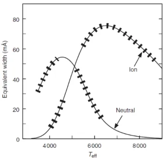
Therefore, neutral species are strengthened with temperature, due to the increased likelihood of excitations, until the thermal energy becomes comparable to the ionization potential. Eventually, the lines from singly ionized elements are weakened too when most absorbers become doubly ionized, and so forth.

Figure 2.2 Temperature dependence of weak metal lines. The strength of neutral species increases with

temperature before becoming singly ionized, at which point their ionic counterparts begin to increase until they

are overtaken by the next ionization stage. Credit: Gray 2005(reproduced and adapted with permission).

2.2.2

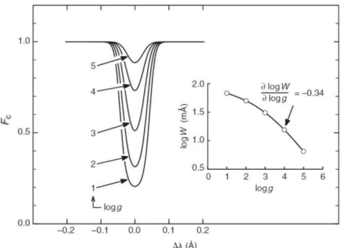
... gravity

The principle of gravity, g, dependence can be laid out similarly as for the temperature. Under the assumption of hydrostatic equilibrium, the gas pressure is approximately

P_g ∝ g2/3. (2.23)

Combined with the ideal gas law, it can be related to the electron pressure. In the high-temperature limit, all hydrogen is ionized, yielding about twice as many particles in total as free electrons,

P_g ≈2Pe; (higher T ) (2.24a)

in temperature regimes where, instead, Pe Pg, the relation reduces to

P_g ∝ Pe2. (lower T ) (2.24b)

To evaluate line strengths, it is important to assess the surroundings of the absorber. First, we consider weak lines. If the line species X has most of its element in the next ionization stage, it follows from Eq. (2.21) that

lλ ∝ N_X ∝ N_X+Pe, (2.25)

where NX+ is almost the total number density of the element and thus considered constant. When dividing the line and continuum absorptions, the electron pressures cancel, indicating an invariance to changes in gravity. If, on the other hand, the species has most of its element in the same ionization

Figure 2.3 Gravity dependence of an FeII line. At Solar temperatures, as in this example, iron is mostly

ionized. Thus, the modeled change in equivalent width is consistent with the exponent in Eq. (2.26). Credit:

Gray 2005 (reproduced and adapted with permission).

stage, then lλ κλ ∝ Pe−1∝ g −_1/3 , (2.26)

with the last step making use of Eqs. (2.23) and (2.24b).

Strong lines follow the same analysis, with the exception of additional gravity dependence in-troduced via αλ in Eq. (2.19). It can be shown that for e.g. quadratic Stark and van der Waals

broadening γ4∝ Pe and γ6∝ Pg. The dominating term governs the resulting dependence, which is

best studied in the wings of strong lines.

2.2.3

... metallicity

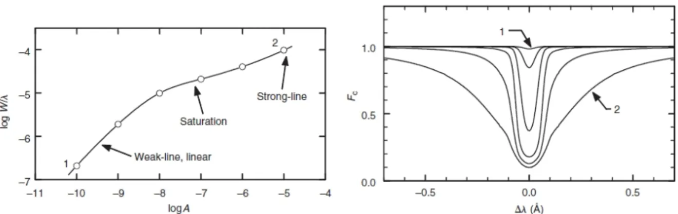
Considering the chemical abundance of some element X relative to hydrogen,

A_X = N_X/N_H, (2.27)

the change in equivalent width with A is called a curve of growth (Fig. 2.4). A weak line, dominated by the Doppler core, exhibits linear growth,

W ∝ A. (weak) (2.28a)

The line is said to be saturated when the central depth approaches its maximum, after which the growth is slowed down,

W ∝?A, (strong) (2.28b)

and allocated to the wings.

Figure 2.4 Curve of growth. The circles at different abundances (left) correspond to the shown line profiles

(right). Credit: Gray 2005 (reproduced and adapted with permission).

it will increase in lock-step with other metallic elements, i.e. prominent electron donors. Continuous absorption, through its dependence on Pe, consequently delays the growth curve. The metallicity,

defined as the logarithmic iron abundance relative to the Sun,

[Fe/H] = log AFe−log AFe,@, (2.29)

becomes a measure through which all other metals may be scaled.

2.3

Instrumentation

The following subsections, which cover the elementary aspects of spectroscopic instrumentation, are based on the textbooks by Chromey (2010) and Kitchin (2013).

2.3.1

Spectrographs

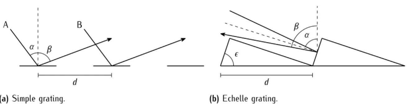
The principles of a diffraction grating is based on the interference of light. Considering a reflection grating with facet separation d, as in Fig. 2.5a, one could trace the paths of two rays, A and B, of the same wavelength. Incident at an angle α and reflected at −β, measured counter-clockwise from the grating normal, the rays interfere constructively when their path difference is an integer multiple of the wavelength,

d(sin α + sin β) = mλ, m ∈ Z (2.30)

known as the Grating Equation, with m denoting the spectral order. However, the configuration described above entails three primary issues:

1. A significant amount of the incoming light is blocked, and thus lost, in-between facets. 2. IfEq. (2.30) is differentiated to obtain the angular dispersion,

dβ dλ =

m

A B

d α _β

(a)Simple grating.

d

α β

ε

(b) Echelle grating.

Figure 2.5Different types of diffraction gratings.

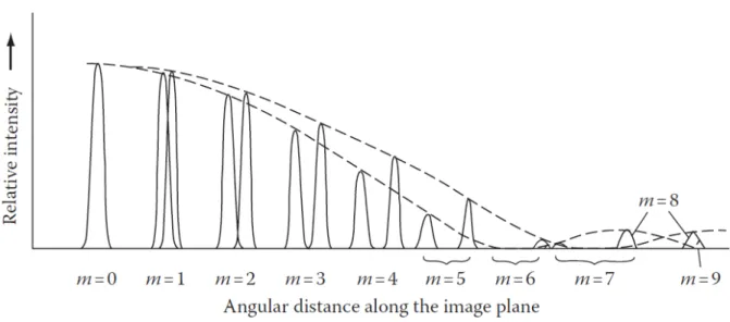
it becomes evident that no dispersion occurs in the zeroth order, which is also the order with highest efficiency.

The intensity distribution along the image plane θ (related to the predefined angles through sin θ = sin α + sin β) is given by, I(θ) = I₀« sin 2`<sub>πDsin θ</sub> λ ˘ `_{πDsin θ} λ ˘2 ff « sin2`<sub>Nπdsin θ</sub> λ ˘ sin2`_πdsin θ λ ˘ ff , (2.32)

where I0 is the central intensity, N the number of facets, and D the width of the feeding slit or fiber. The

expression inside the first pair of square brackets, known as the blaze function, modulates the diffraction pattern, providing maximum intensity when θ = 0 ⇒ α = −β ⇒ m = 0.

3. Some wavelengths λm and λn from spectral orders m and n, respectively, will be superimposed

if they satisfy mλm= nλn, causing overlap between neighboring regions. The unique interval

for any given m, called the free spectral range (FSR), becomes ∆λFSR = λmax

m+ 1, (2.33)

where λmax is the largest wavelength which the spectrograph can record.

The solution to issues 1 and 2, concerning the light loss, is found through a blazed grating. By introducing a periodically saw-toothed structure, inclined at an angle ε to the plane of the grating, much more of the light can be retained. Simultaneously, the blaze function is shifted toward m > 0. Gratings operating at ε near 90◦ _{are called echelles, and are suitable for observing high orders. From}

Eq. (2.31)follows that the resolution, δλ, i.e. the smallest distinguishable separation of wavelengths, improves with higher m. A related quantity is the resolving power, R, defined as the reciprocal relative resolution; it can be shown that

R = λ

δλ = mN. (2.34)

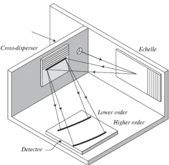
The solution to the 3rd_{issue, crucial for high-resolution spectroscopy where the FSR becomes notably} limited, is the introduction of a cross-disperser, which separates the orders in a direction perpendicular to the diffraction. Placed after the grating, the cross-disperser is usually a prism; the combination is referred to as a grism.

Figure 2.6 Bichromatic intensity distribution for a diffraction grating. The angular dispersion increases with

spectral order; at m = 7, adjacent orders begin to overlap. The dashed curve outlines a non-blazed modulation. Credit: Kitchin 2013(reproduced with permission).

Echelles are not entirely unproblematic. The steep angle requires the device to be mounted close to the Littrow configuration, in which the incident light is parallel to the facet normal, to avoid shadowing effects. Furthermore, prism aberrations cause the output spectra to be curved and misaligned with an orthogonal grid of pixels.

2.3.2

Detectors

The detector is a device onto which the produced spectra are recorded, and the currently preferred choice among astronomers is the charged-coupled device (CCD). A CCD camera consist of an array of pixels, each equipped with a capacitor in which the semiconductor is most often a layer of silicon. As incident light produces photoelectrons, they become stored in the potential well of each capacitor. After an exposure is terminated, the charges are shifted row by row—known as charge coupling—and converted to a signal through an analog-to-digital converter (ADC).

The signal is registered in analog-to-digital units (ADUs), and the gain of a CCD specifies the number of electrons needed to increase the output by one unit. This is due to the full well size of a pixel being on the order of ∼ 105 _{electrons, whereas the ADC is usually limited to 16-bit} data (corresponding to 216_{= 65 536 values). If the target is sufficiently luminous, the response of the} detector will be linear, i.e. the output signal will be proportional to the input illumination. Saturation could cause so-called blooming, where electrons spill over to adjacent pixels.

The quantum efficiency (QE), i.e. the registered fraction of incoming photons, of modern CCDs can reach 95 % for wavelengths λ < 1.1 µm below the silicon band gap, making them ideal for observations in the optical and near-infrared (NIR).

Figure 2.7 Schematic view of an echelle grating with a cross-disperser. The spectral orders are shown to be

spatially separated when reaching the detector. Credit: Chromey 2010 (reproduced with permission).

2.3.3

Noise

A perfect detector is never noise-less. The counting of photons (or equivalently, photoelectrons) as independently occurring events is well-described by Poisson statistics. For such a distribution, there exists an inherent uncertainty associated with the number of events, N,

σ =?N. (2.35)

In the ideal case, the signal-to-noise ratio (SNR) is equal to the noise, SNR = N

σ =

?

N. (2.36)

CCDs are prone to additional noise. If not cooled enough, thermally agitated electrons—known as dark currents, because they can be detected with the shutter closed—degrades the signal. Conversely, temperatures close to absolute zero slow down the diffusion of charges during transfer; the added read-out noise is proportional to the pixel sampling frequency. Scientific-grade detectors, for which the total read-out time may be several seconds, counteract this by being assembled in mosaics of multiple CCDs, each with its own register.

Chapter 3

Methods

3.1

Target selection

This work makes use of data from the HARPS (High-Accuracy Radial Velocity Planet Searcher;

Mayor et al. 2003) cross-dispersive echelle spectrograph, installed on the ESO (European Southern Observatory) 3.6 m Telescope at La Silla, Chile. HARPS has a resolving power of R = 115 000 and its detector is divided into two CCDs, dubbed the BLUE and RED modes, covering a spectral range of λ = 378 − 530 nm (m = 161 − 116) and λ = 533 − 691 nm (m = 114 − 89), respectively.

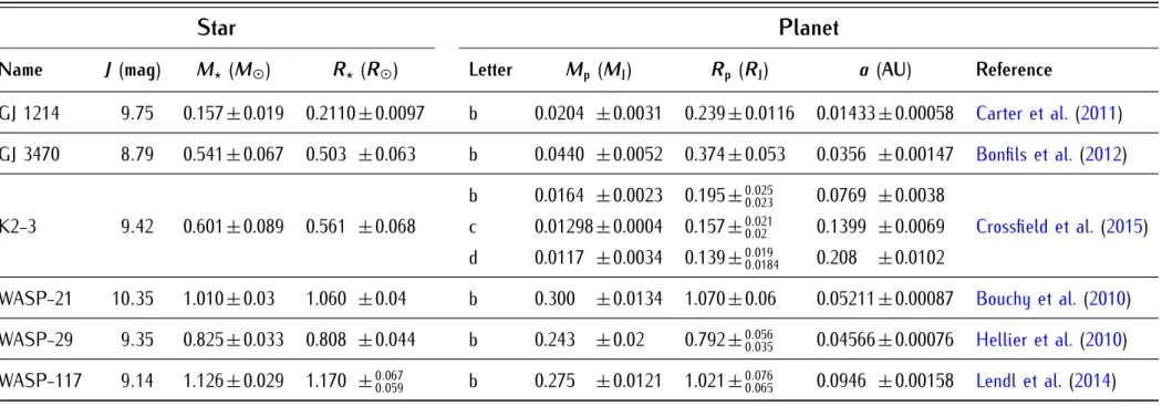
All target stars (listed inTable 3.1) are hosts to at least one confirmed exoplanet each, for which transit observations with HARPS are available. They have been selected to represent a range in late spectral types on the main sequence as well as in companion masses and sizes, while additionally having sufficiently bright J-band magnitudes.

3.2

Data processing

The interface of the ESO Archive Science Portal1_{allows the user to sort available HARPS} observa-tions by SNR. For each target, the Nobs= 10 data sets with highest SNR are downloaded from the ESO Science Archive Facility2 _{(seeAppendix A).}

Before any analysis can commence, the raw data must be adjusted for unwanted influences and conveniently formatted. This processing is performed in multiple steps, which are detailed below in separate subsections.

3.2.1

Reduction

Data reduction is the collective name for the correction of bias, flat fielding and dark currents; in spectroscopy, it also involves the extraction of spectral orders, all of which is performed with the

1_{Available athttp://archive.eso.org/scienceportal.}

Table 3.1Target stars and their planets. The stars are listed alphabetically after their catalog or mission name, and the planets are assigned letters (starting with ‘b’)

ordered after their discovery or distance from the host star if several are discovered simultaneously. Stellar/planetary masses and radii are given in Solar/Jovian units.

Star

Planet

Name J (mag) M? (M@) R? (R@) Letter Mp (MJ) Rp (RJ) a(AU) Reference

GJ 1214 9.75 0.157±0.019 0.2110±0.0097 b 0.0204 ±0.0031 0.239±0.0116 0.01433±0.00058 Carter et al. (2011) GJ 3470 8.79 0.541±0.067 0.503 ±0.063 b 0.0440 ±0.0052 0.374±0.053 0.0356 ±0.00147 Bonfils et al.(2012) b 0.0164 ±0.0023 0.195±0.025 0.023 0.0769 ±0.0038 K2-3 9.42 0.601±0.089 0.561 ±0.068 c 0.01298±0.0004 0.157±0.021 0.02 0.1399 ±0.0069 Crossfield et al.(2015) d 0.0117 ±0.0034 0.139±0.019 0.0184 0.208 ±0.0102

WASP-21 10.35 1.010±0.03 1.060 ±0.04 b 0.300 ±0.0134 1.070±0.06 0.05211±0.00087 Bouchy et al. (2010)

WASP-29 9.35 0.825±0.033 0.808 ±0.044 b 0.243 ±0.02 0.792±0.056

0.035 0.04566±0.00076 Hellier et al. (2010) WASP-117 9.14 1.126±0.029 1.170 ±0.067

REDUCE (Piskunov & Valenti 2002) package. For each night of observation, the calibration files are obtained from the preceding evening.

The bias level is the intrinsic signal from a zero-time exposure. Several frames are combined to create a master bias, which is subtracted from the raw data. Furthermore, pixels may exhibit sensitivity variations, compensated by sampling some uniform light source to create a flat field, with which the resulting frame from the previous step is divided. Dark currents are not an issue for HARPS which is temperature-controlled and isolated in a vacuum vessel.

3.2.2

Wavelength calibration

After the extraction of spectral orders, each pixel must be assigned a specific wavelength. The calibration is done by illuminating the CCD with a lamp containing elements, commonly thorium-argon, with accurately measured emission lines.

Each data set then consist of 2D arrays for the physical quantities, where the columns corre-spond to wavelengths and the rows to spectral orders. The following notation will be used: λk

i,j

is the wavelength at pixel i = 0, 1, ..., Npix−1 and order index j = 0, 1, ..., Nord−1 of observation

k= 1, 2, ..., N_obs, and F(λk

i,j) is the flux at that point.

3.2.3

Summation

The Nobs sets should be combined to yield a higher SNR, however, the summation cannot be applied straightforward since at each time of observation the Earth has a different radial velocity component in the direction of the target.

Firstly, the wavelengths are transformed from the observatory reference frame to the barycentric frame of the Solar System through a Doppler shift,

λbary = λobs ´ 1 + vbary c ¯ , (3.1)

where vbary is the barycentric correction reaching a maximum value of

v_bary ≤2π(1 AU/yr + RC/(24 h)) ≈ 30 km/s, (3.2) where the two terms account for the Earth’s orbit around the Sun and rotation around its own axis. This is significant compared to the resolution of HARPS, able to detect variations down to

v_lim = c∆λ λ =

c

R ≈3 km/s. (3.3)

The reason for transforming to the barycentric frame is that the radial velocity of the target remains constant, neglecting the influence of its planetary system, which could be on the order of ∼ 0.1 km/s, assuming a stellar mass of M?= 1 M@, a planetary mass of Mp= 1 MJ and a semi-major axis of

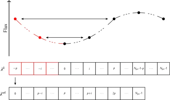
Flux

λk

λref

−p · · · −i · · · ₀ · · · i · · · p · · · Npix-1-p · · · Npix-1

0 · · · p−i · · · p · · · p+i · · · 2p · · · Npix-1

Figure 3.1Padded spectrum. The illustration showcases the kth observation of a target being padded in order

to resemble the reference scale. The arrays at the bottom indicate the pixel indices. Note that λk

−p is not

necessarily equal to λref

0 , but rather sufficiently close for Bézier interpolation to remain well-behaved.

For a star-planet system, the orbital radius of the star, around the common center of mass, is given by

r?= a M_p M?+ Mp

. (3.4)

If the orbit is approximated to a circle, the stellar velocity is easily calculated with

v?=2πr?

P , (3.5)

where P is the period obtained from Kepler’s Third Law:

a3 P2 =

G(M?+ Mp)

4π2 . (3.6)

Secondly, the discrete barycentric wavelengths are different for each data set. Therefore, the wavelength scale of the first observation is chosen as a reference onto which the succeeding ob-servations are interpolated. In order to avoid diverging extrapolation, the spectra are also mirrored around the out-of-bound endpoints (see Fig. 3.1), i.e. the p padded points extending the blueward end become

λk−i,j = 2λk0,j− λki,j, ∀i = 1, 2, ..., p (3.7a)

F(λk_−i,j) = F(λk_i,j), (3.7b)

The total spectrum is finally given by F_tot(λi,j) = N_obs X k=1 Fk(λrefi,j), (3.8)

where Fk(λrefi,j) is the flux of the kth observation interpolated onto the wavelengths λrefi,j of the reference

scale. Following a similar treatment, the propagation of errors is given by

σ_tot(λi,j) = g f f e N_obs X k=1 σ_k2(λrefi,j). (3.9)

3.2.4

Continuum normalization

Conventionally, a spectrum is normalized with respect to its continuum C(λ),

Fc(λ) = F(λ)

C(λ), (3.10)

rendering wavelength regions void of spectral lines equal to unity and facilitating the measurement of relative line strengths.

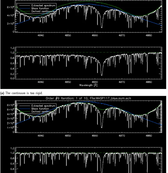
As a first approximation, stellar continua should resemble black-body curves, however, the com-posite spectrum of an echelle spectrograph appears quite different. Due to the blaze function, the intensity of each spectral order peaks around its central wavelength. To compensate for this (and to also avoid gaps in the spectrum), the grating is usually constructed such that neighboring orders partially overlap, causing additional inconsistencies when co-adding their contributions (seeFig. 3.2). Finding C(λ) becomes a numerical effort, with visual assessment needed to determine the rigidity of the fit; it should not forfeit large-scale details by being too exaggerated, nor sink into small-scale details by being too relaxed. Furthermore, telluric emission lines can cause local augmentations, and intervals to be ignored are manually selected around them.

3.2.5

SNR filtration

Following Poisson statistics, the SNR of the summed spectrum is expected to increased by a factor of ?

N_obs (given that all observations have approximately equal exposure times) relative to the average

SNR of its individual observations,

SNRavg = 1 N_obs N_obs X k=1 SNRk. (3.11)

The presence of read-out noise mitigates the sought increase, which can be elevated by filtering out noisy spectral orders. This is done by only retaining the orders j0 _{with an average SNR higher than}

(a)The continuum is too rigid.

(b)The continuum is too relaxed.

Figure 3.2 Incorrect continuum normalization. The upper panels show the spectrum (white) in ADUs, together

with the blaze function (blue). In order to follow the curvature of overlapping orders, the rigidity of the derived continuum (green) must be tuned in-between the extremes above. Lines with strong wings are often helpful,

as with Hβ to the center-right.

the arbitrarily set threshold at 90 % of the SNR of all orders, in each respective mode, 1 N_pix N_Xpix−1 i=0 F_tot(λi,j0) σ_tot(λi,j0) > 0.9 N_pixN_ord N_Xpix−1 i=0 NX_ord−1 j=0 F_tot(λi,j) σ_tot(λi,j) . (3.12)

Table 3.2 Signal-to-noise ratios. All values are averages of the RED and BLUE modes, except SNR_tot and

f_SNR for M-stars, which only comprise RED values.

Star SNRavg SNRtot fSNR

GJ 1214 6.4 66.8 3.3 GJ 3470 12.6 90.5 2.3 K2-3 26.6 132.5 1.6 WASP-21 32.4 109.2 1.1 WASP-29 25.9 81.3 1.0 WASP-117 57.0 148.5 0.8

Additionally for M-stars, the BLUE mode is entirely omitted since in most cases SNRk,BLUE<10.

The total calculated SNR becomes,

SNRtot = 1 N_pixN_ord0 N_Xpix−1 i=0 N0 ord−1 X j0₌₀ F_tot(λi,j0) σ_tot(λi,j0) , (3.13) where N0

ord is the number of retained orders.

Subsequently, one is then able to construct an enhancement factor for the SNRs,

f_SNR = ? SNRtot

N_obsSNR_avg, (3.14)

indicative of how much the signal improved—or worsened, if the factor is less than 1—compared to theory.

3.3

Spectral synthesis

Line data for the trimmed wavelength intervals are obtained from the The Vienna Atomic Line Database3 _{(VALD; Piskunov et al. 1995; Ryabchikova et al. 2015). The ‘Extract Stellar’ query is} configured to include van der Waals broadening from the theory by Anstee-Barklem-O’Mara (ABO; see Barklem et al. 1998, and references therein).

Stellar parameters are derived using Spectroscopy Made Easy4_{(SME;Valenti & Piskunov 1996;}

Piskunov & Valenti 2017), which is an interface-based software. SME performs spectral synthesis by solving the equilibrium number densities of absorbers, needed for calculating opacities. Together with a model photosphere, the radiative transfer equation can be iteratively solved and disc-integrated to provide a flux spectrum. To find the parameters best matching with observations, SME interpolates from a grid of e.g. MARCS (Gustafsson et al. 2008) model photospheres, with which χ2_{-minimization is} performed. An initial guess for the stellar parameters of each targets is retrieved from the Exoplanet

3_{Available at i.a. http://vald.astro.uu.se.}

(a)The initial guesses (red) span a range of 1200 K in T_eff,

0.5 dex in log g, and 1 dex in [Fe/H] (denoted as [M/H]). (b)along all three axes, showcasing the robustness of SME.Close-up of the results (blue), which have a small spread

Figure 3.3 SME convergence test. To illustrate the optimization capability of SME, regardless of initial

estimates, 1000 tests of the Sun’s reflection off asteroid Vesta were carried out across the parameter space. Credit: Piskunov & Valenti 2017(reproduced with permission).

Data Explorer5 _{(EDE), or estimated from the most resembling sample star in Lindgren & Heiter} (2017). Although, the closeness of the initial guess should not be crucial, as the convergence of SME has been shown to be accurate for a wide range of reasonable values (see Fig. 3.3).

Via the graphical user interface (GUI), one can create a mask distinguishing line from continuum points, but also wavelength intervals to be ignored during fitting, which is implemented for observed lines not found in the line list and the cores of strong lines without available non-LTE (NLTE) correction.

Chapter 4

Results

4.1

Observed and synthetic spectra

Prior to the spectral synthesis, the post-processed data should be previewed to verify that all steps have been void of critical errors. Fig. 4.2shows a smoothed composition of observations. Ordered after spectral type, the diminishing of Balmer lines becomes evident, as does the wide spread of metallic and molecular lines. On the redward end can be seen the constant presence of contamination by telluric oxygen. Another noticeable aspect is the result of the SNR filtration, which has removed the noisiest regions, most obvious in the BLUE orders.

5160 5170 5180 5190 5200 5210 0.0 0.2 0.4 0.6 0.8 1.0 C2 1 5159.039 C2 1 5159.053 C2 1 5159.186 C2 1 5159.939 C2 1 5159.990 C2 1 5160.098 Fe 1 5160.494 C2 1 5160.877 C2 1 5160.902 C2 1 5161.032 C2 1 5161.642 C2 1 5161.709 C2 1 5161.819 C2 1 5162.456 C2 1 5162.486 C2 1 5163.110 C2 1 5163.170 Fe 1 5163.710 C2 1 5163.775 C2 1 5164.305 Fe 1 5166.849 Fe 1 5167.721 Mg 1 5168.761 Fe 1 5168.927 Ni 1 5170.099 Fe 1 5170.337 Fe 2 5170.468 Fe 1 5173.037 Fe 1 5173.112 Mg 1 5174.125 Ni 1 5174.309 Ti 1 5175.184 Ni 1 5178.002 Fe 1 5178.675 La 2 5184.854 Mg 1 5185.048 Ti 2 5185.155 Fe 1 5185.710 Fe 1 5185.710 Ni 1 5186.003 Fe 1 5187.169 Ti 2 5187.346 Ce 2 5188.903 Fe 1 5189.359 Ti 2 5190.132 Ca 1 5190.289 Nd 2 5192.886 Fe 1 5192.900 Zr 2 5193.038 Fe 1 5193.789 Ni 1 5193.941 Nd 2 5194.056 Ti 1 5194.415 Cr 1 5194.938 Fe 1 5196.388 Fe 1 5196.918 Fe 1 5197.506 Mn 1 5198.037 Fe 2 5199.015 Fe 1 5200.158 Nd 2 5201.569 Y 2 5201.858 Fe 1 5203.704 Fe 1 5203.784 Cr 1 5205.947 Fe 1 5206.032 Y 2 5207.172 Cr 1 5207.473 Cr 1 5209.859 Fe 1 5210.044 Ti 1 5211.835 Ti 2 5212.981 Nd 2 5213.811 Cr 1 5215.583 5160 5170 5180 5190 5200 5210 Wavelength 0.0 0.2 0.4 0.6 0.8 1.0 Intensity WASP117_blue_fig

Figure 4.1Example SME synthesis. The staring synthesis (green) is optimized with respect to the observations

4000

5000

6000

7000

(Å)

No

rm

ali

ze

d f

lux

K H

G

H

Fe

H

Fe

Mg

D

+D

Ca

TiO

H

GJ 1214

GJ 3470

K2-3

WASP-29

WASP-21

WASP-117

Retained

Removed

Figure 4.2Composite spectra of targets. The vacuum wavelengths are in the rest frames of the stars. Smoothing

has been applied to distinguish characteristic features. The BLUE and RED modes constitute the left and right

halves, respectively. The black-colored sections are kept orders satisfying the criterion inEq. (3.12), whereas

red-colored parts are subsequently trimmed off. Prominent spectral lines are indicated by their Fraunhofer names or spectroscopic notation; the TiO marker is placed at the center of its molecular band.

4.2

Derived parameters

The outcome from the spectral fitting described in Sect. 3.3 is presented in Table 4.1. In the applied MARCS models, the micro- and macroturbulence are fixed as vmic= 1 km/s and vmac= 3 km/s, respectively, similar to values adopted by Valenti & Fischer (2005). Whereas the rotational velocity of the stars is assumed negligible and set to zero. To mimic the instrumental profile of HARPS, the syntheses are additionally convolved with a corresponding point spread function (PSF). The abundances of elements with strong lines in the studied regions are identified and also set as free parameters, in order compensate for insufficient growth from the metallicity scaling. In Fig. 4.3, the derived parameters and their uncertainties are compared to previous studies of the same stars from the literature.

4.3

Limb darkening

The derived parameters are thereafter used to compute new MARCS model photospheres, for more accurate retrieval of specific intensities compared to interpolation in a grid of pre-existing models. For stars with dual modes, the new models use parameter averages. The specific intensities are calculated at 49 (the maxmimum number of points allowed by SME) equidistant µ-values between 1 and 1/49 ≈ 0.02 across each stellar disc. Assuming a quadratic limb darkening of the form

Iλ(µ)

Iλ(1) = 1 − a(1 − µ) − b(1 − µ)

2_{, (4.1)}

regression is applied to find the limb darkening coefficients (LDCs), a and b, for a subset of the evaluated wavelengths, shown in Fig. 4.4. Although the coefficients exhibit a global trend, points which coincide with the cores of strong lines are scattered due to their shallow depth of formation.

Table 4.1 Derived stellar parameters and abundances. The stars are sorted after their spectral types listed on SIMBADa. Abundances are given as logarithmic number

densities relative to the total, e.g. log (NMg/Ntot) for Mg.

BLUE

RED

Star Sp. type Teff (K) log g [Fe/H] Mg Teff (K) log g [Fe/H] Na Ca

WASP-117 F9 V 5872±229 4.19±0.81 −0.32±0.18 −4.51±1.49 6045±257 4.40±0.83 −0.17±0.19 −5.95±0.11 WASP-21 G3 V 5801±172 4.21±0.66 −0.59±0.15 −4.21±0.82 5885±280 4.37±1.16 −0.47±0.20 −5.88±0.24 WASP-29 K4 V 5180±303 4.69±0.61 0.28±0.58 −3.73±0.38 4486±198 4.36±0.67 −0.36±0.25 −5.86±0.13 −5.64±0.35 K2-3 M0 V 3718±105 4.82±0.88 −0.47±0.11 −5.91±0.17 GJ 3470 M2 V 3305±107 4.25±0.97 −0.73±0.11 −5.78±0.31 GJ 1214 M5 V 2854± 71 3.22±1.36 −1.20±0.15 −6.87±0.28 a_{Available athttp://simbad.u-strasbg.fr/simbad.}

3.0 3.5 4.0 4.5 5.0 5.5 6.0 Teff (kK): This work

3.0 3.5 4.0 4.5 5.0 5.5 6.0 Teff ( kK ): O th er s' w or k 2.0 2.5 3.0 3.5 4.0 4.5 5.0 5.5 logg: This work

2.0 2.5 3.0 3.5 4.0 4.5 5.0 5.5 lo gg : O th er s' w or k -0.8 -0.6 -0.4 -0.2 0.0 0.2 0.4 [Fe/H]: This work

-0.8 -0.6 -0.4 -0.2 0.0 0.2 0.4 [F e/ H ]: O th er s' w or k

Figure 4.3 Comparison with previous studies. The horizontal axis shows the (BLUE + RED averaged) values

and errors of this work (from Table 4.1), whereas the vertical axis shows previously determined parameters

for the same stars retrieved from the references in Table 3.1. The dotted line indicates a 1:1 relationship.

Surface gravities were unavailable for GJ 3470 and K2-3, and are instead calculated with g = g@M?/R?2. Two

-0.5 0.0 0.5 1.0 1.5

_WASP-117

_WASP-21

WASP-29

_K2-3

_{GJ 3470}

Figure 4.4 Wavelength dependency of the limb darkening. The quadratic LDCs from Eq. (4.1) are evaluated

for the retained spectral region of each star in steps of 10 Å. The color of each coefficient is indicated on the first subplot.

Chapter 5

Discussion

5.1

Uncertainties

In the SME solver, numerical errors are of little importance. Instead, the uncertainties arise due to deficiencies in the stellar models, which SME tries to estimate through the sensitivities of unmasked points. The parameter changes are inversely proportional to the partial derivatives of the flux with respect to each parameter. Generally, this works well, however, for parameter-insensitive points the uncertainties could diverge, leading to overestimation.

Regarding the quality of derived parameters, the BLUE and RED modes each have their own benefits. While RED mode has a higher SNR for late-type stars, the spectral region of the BLUE mode contains many more gravity-sensitive Fe lines. In the derived set of parameters, the average uncertainties are hσTeffi= 191 K, hσlog gi = 0.88 dex and hσ[Fe/H]i = 0.21 dex. The precision is com-parable to spectroscopic determination of this kind, reflected in the Fig. 4.3 comparison, except for surface gravity which might be overestimated following the discussion above.

5.2

Further improvements

The strive to minimize the difference between observations and syntheses might not be so simple as obtaining additional observations to increase SNR, although admittedly that would help to some extent. One source of several other errors is the inadequacy of the stellar models. The numerical task is made feasible by oversimplifying, at the cost of failure to reproduce finer details in the spectra.

The atomic line properties are constantly updated—experimentally in laboratories and theoret-ically through complex modeling. Moreover, the inclusion of non-‘classical’ effects would noticeably improve the outcome. For example, Zeeman broadening could play a significant role in magnetically active stars. The turbulence scales should preferably also be target specific, or at least be assessed from trends based on the stars’ auxiliary characteristics.

Neither should the computational aspects be neglected. By fitting numerous parameters simul-taneously, there is a risk of degeneracy which could imply the over- or underestimation of some

parameters. Ideally, the partial derivatives of the optimization should be utilized to select wave-lengths regions for which only a subset of the parameters are fitted, to subsequently be used as fixed values in regions suitable for the remaining parameters. Furthermore, the SNR filtration should be evaluated to a non-arbitrary threshold which would not exclude important features while keeping the overall signal statistically significant.

Chapter 6

Conclusion

The task of determining stellar parameters is intricate and involves several steps of data handling. The prerequisites are high-resolution spectra which are accurately pipelined and combined to yield a high SNR. The process that follows is then facilitated with the aid of easily accessed databases, computationally effective stellar models and user-friendly spectroscopy tools.

In this study {Teff, log g, [Fe/H]} of 6 late-type stars were determined, using HARPS data and

χ2-fitting with SME, to a precision suitable for subsequent studies of their companions. Improvements

can be made by considering fine structure effects in the stellar models and through decoupling in the numerical derivation.

The future of exoplanet characterization is worthy of a final word. Although the work presented here has been carried out in the optical regime, the fundamental parameters of an individual star are wavelength-independent and essentially constant at the timescale of planetary transits (given the star’s activity level is not too abnormal). Thus they are a powerful tool and can, for in-stance, be utilized to synthesize spectra for regions containing lines of compounds associated with biosignatures—prospectively detecting them in the atmospheres of ever-smaller exoplanets.

Acknowledgements

I would like to express my deepest gratitude toward Prof. Nikolai Piskunov for his kind mentorship. Your numerous anecdotes from around the globe have persuaded me to explore it for myself.

Thank you to Dr. Bengt Edvardsson for your constructive input on this thesis and for the specific models which were crucial for the project’s completion.

Appendix A

Observations

Table A.1 HARPS observations. The columns specify the object EDE/ESO identifiers, and the ESO IDs for

the program in which the observation was carried out and its unique dataset with timestamp.

Object (EDE/ESO) Program ID Dataset ID

GJ 1214 GJ1214

283.C-5022(A) HARPS.2009-07-27T02:54:44.319HARPS.2009-07-30T00:41:20.581 HARPS.2009-07-30T02:50:18.712 183.C-0437(A) HARPS.2009-08-29T23:28:52.045 HARPS.2009-09-03T23:26:05.655 HARPS.2009-09-24T23:21:36.122 HARPS.2010-04-11T08:07:44.823 HARPS.2011-04-28T05:45:46.770 HARPS.2011-06-16T01:54:17.803 198.C-0838(A) HARPS.2018-03-21T08:59:57.096 GJ 3470 GJ3470 082.C-0718(B) HARPS.2008-12-25T06:38:34.917_{HARPS.2008-12-26T06:34:50.163} 183.C-0437(A) HARPS.2011-01-05T05:13:42.300_{HARPS.2012-05-12T22:37:16.723}

198.C-0838(A) HARPS.2016-10-28T08:21:45.774 HARPS.2016-11-06T08:34:57.913 HARPS.2016-11-09T08:34:40.547 HARPS.2016-11-11T08:30:14.994 HARPS.2017-04-12T00:17:39.549 HARPS.2018-03-22T02:04:03.171 K2-3 2M1129−0127 191.C-0873(A) HARPS.2015-05-04T00:51:10.497 HARPS.2016-02-02T06:06:44.049 HARPS.2016-02-03T06:09:07.758 HARPS.2016-02-04T05:50:22.869 HARPS.2016-02-05T06:02:06.439 HARPS.2016-02-06T05:30:57.447 HARPS.2016-02-28T03:58:22.504 HARPS.2016-03-05T03:45:35.537 HARPS.2016-03-06T03:56:04.084 198.C-0838(A) HARPS.2017-02-06T08:18:37.443

WASP-21 SW2309+1823 072.C-0488(E) HARPS.2008-08-31T06:00:07.132 082.C-0608(A) HARPS.2008-10-15T03:03:34.833 HARPS.2008-10-16T03:33:47.405 HARPS.2008-10-21T02:51:03.797 HARPS.2008-10-22T02:42:32.846 HARPS.2008-10-24T01:57:51.504 HARPS.2009-10-07T02:55:39.881 HARPS.2009-10-08T02:52:32.865

084.C-0185(E) HARPS.2009-10-09T02:35:54.999_{HARPS.2009-10-12T02:56:47.280}

WASP-29 SW2351−3954 085.C-0393(A) HARPS.2010-09-05T09:21:56.485 099.C-0898(A) HARPS.2017-08-18T03:38:17.703 HARPS.2017-08-18T03:53:49.064 HARPS.2017-08-18T04:24:51.077 HARPS.2017-08-18T04:40:22.089 HARPS.2017-08-18T05:57:57.105 HARPS.2017-08-18T06:13:28.076 HARPS.2017-08-18T06:28:59.158 HARPS.2017-08-18T06:44:31.099 HARPS.2017-08-18T07:00:03.141 WASP-117 SW0227−5017 094.C-0090(A) HARPS.2014-10-24T01:41:59.564 HARPS.2014-10-24T02:02:31.934 HARPS.2014-10-24T04:58:44.926 HARPS.2014-10-24T05:29:49.926 HARPS.2014-10-24T06:16:24.946 HARPS.2014-10-24T06:31:57.037 HARPS.2014-10-24T07:18:35.938 HARPS.2014-10-24T07:34:08.387 HARPS.2014-10-24T07:49:39.907 HARPS.2014-10-24T08:05:13.417

Bibliography

Adibekyan, V., Sousa, S. G. & Santos, N. C. (2018), Characterization of Exoplanet-Host Stars, in T. L. Campante, N. C. Santos & M. J. P. F. G. Monteiro, eds, ‘Asteroseismology and Exoplanets’, Springer.

Aronson, E. & Waldén, P. (2015), ‘Using near-infrared spectroscopy for characterization of transiting exoplanets’, Astron. Astrophys. 578, A133. DOI: 10.1051/0004-6361/201424058

Barklem, P. S., Anstee, S. D. & O’Mara, B. J. (1998), ‘Line Broadening Cross Sections for the Broadening of Transitions of Neutral Atoms by Collisions with Neutral Hydrogen’, Publ. Astron.

Soc. Aust. 15, 336. DOI: 10.1071/AS98336

Bonfils, X., Gillon, M., Udry, S. et al. (2012), ‘A hot Uranus transiting the nearby M dwarf GJ 3470’,

Astron. Astrophys. 546, A27. DOI: 10.1051/0004-6361/201219623

Bouchy, F., Hebb, L., Skillen, I. et al. (2010), ‘WASP-21b: a hot-Saturn exoplanet transiting a thick disc star’, Astron. Astrophys. 519, A98. DOI: 10.1051/0004-6361/201014817

Böhm-Vitense, E. (1989), Introduction to Stellar Astrophysics, Vol. 2, Cambridge University Press. Carroll, B. W. & Ostlie, D. A. (2017), An Introduction to Modern Astrophysics, 2nd _{edn, Cambridge}

University Press.

Carter, J. A., Winn, J. N., Holman, M. J. et al. (2011), ‘The Transit Light Curve Project. XIII. Sixteen Transits of the Super-Earth GJ 1214b’, Astrophys. J. 730, 82. DOI:

10.1088/0004-637x/730/2/82

Chromey, F. R. (2010), To Measure the Sky, 1st _{edn, Cambridge University Press.}

Crossfield, I. J. M., Petigura, E., Schlieder, J. E. et al. (2015), ‘A Nearby M Star with Three Transiting Super-Earths Discovered by K2’, Astrophys. J. 804, 10. DOI: 10.1088/0004-637x/804/1/10

Gray, D. F. (2005), The Observation and Analysis of Stellar Photospheres, 3rd _{edn, Cambridge} University Press.

Gustafsson, B., Edvardsson, B., Eriksson, K. et al. (2008), ‘A grid of MARCS model atmospheres for late-type stars’, Astron. Astrophys. 486, 951. DOI: 10.1051/0004-6361:200809724

Hellier, C., Anderson, D. R., Collier Cameron, A. et al. (2010), ‘WASP-29b: A Saturn-sized Transiting Exoplanet’, Astrophys. J. Lett. 723, L60. DOI: 10.1088/2041-8205/723/1/l60

Kitchin, C. R. (2013), Astrophysical Techniques, 6th _{edn, CRC Press.}

Lendl, M., Triaud, A. H. M. J., Anderson, D. R. et al. (2014), ‘WASP-117b: a 10-day-period Saturn in an eccentric and misaligned orbit’, Astron. Astrophys. 568, A81. DOI:

10.1051/0004-6361/201424481

Lindgren, S. & Heiter, U. (2017), ‘Metallicity determination of m dwarfs: Expanded pa-rameter range in metallicity and effective temperature’, Astron. Astrophys. 604, A97. DOI:

10.1051/0004-6361/201730715

Mayor, M., Pepe, F., Lovis, C., Queloz, D. & Udry, S. (2008), The quest for very low-mass planets,

in M. Livio, K. Sahu & J. Valenti, eds, ‘A Decade of Extrasolar Planets around Normal Stars’,

Cambridge University Press.

Mayor, M., Pepe, F., Queloz, D. et al. (2003), ‘Setting New Standards with HARPS’, The Messenger

114, 20. ADS: 2003Msngr.114...20M

Mihalas, D. (1970), Stellar Atmospheres, 1st _{edn, W. H. Freeman & Co.}

Piskunov, N. E., Kupka, F., Ryabchikova, T. A. et al. (1995), ‘VALD: The Vienna Atomic Line Data Base’, Astron. Astrophys. Suppl. Ser. 112, 525. ADS: 1995A&AS..112..525P

Piskunov, N. E. & Valenti, J. A. (2002), ‘New algorithms for reducing cross-dispersed echelle spectra’,

Astron. Astrophys. 385, 1095. DOI: 10.1051/0004-6361:20020175

Piskunov, N. & Valenti, J. A. (2017), ‘Spectroscopy Made Easy: Evolution’, Astron. Astrophys.

597, A16. DOI: 10.1051/0004-6361/201629124

Ryabchikova, T., Piskunov, N., Kurucz, R. L. et al. (2015), ‘A major upgrade of the VALD database’,

Phys. Scr. 90, 054005. DOI:10.1088/0031-8949/90/5/054005

Santos, N. C., Israelian, G. & Mayor, M. (2004), ‘Spectroscopic [Fe/H] for 98 extra-solar planet-host stars’, Astron. Astrophys. 415, 1153. DOI: 10.1051/0004-6361:20034469

Unsöld, A. (1955), Physik der Sternatmosphären, Springer.

Valenti, J. A. & Fischer, D. A. (2005), ‘Spectroscopic Properties of Cool Stars (SPOCS). I. 1040 F, G, and K Dwarfs from Keck, Lick, and AAT Planet Search Programs’, Astrophys. J. Suppl. Ser.

159, 141. DOI: 10.1086/430500

Valenti, J. A. & Piskunov, N. (1996), ‘Spectroscopy made easy: A new tool for fitting observations with synthetic spectra’, Astron. Astrophys. Suppl. Ser. 118, 569. DOI: 10.1051/aas:1996222