Life cycle cost analysis of the ventilation system in Stockholm's road tunnels

(1)

Journal of Quality in Maintenance Engineering

Life cycle cost analysis of the ventilation system in Stockholm’s road tunnels

Journal: Journal of Quality in Maintenance Engineering Manuscript ID JQME-05-2017-0032.R2

Manuscript Type: Research Paper

Keywords: Capital equipment, Economic replacement time, Life cycle cost analysis, Maintenance, Optimization model, Ventilation system

(2)

Journal of Quality in Maintenance Engineering

Life cycle cost analysis of the ventilation system in Stockholm’s road

tunnels

Abstract

Swedish Transport Administration (Trafikverket) invests millions of dollars, into its annual budgets to purchase heavy equipment. Given the enormous costs of acquiring, operating and maintaining these assets, it is important to optimise their replacement.

This study presents a practical economic replacement decision model to identify the economic lifetime of the ventilation system used by Trafikverket in its Stockholm tunnels. The proposed data driven optimisation model considers operating and maintenance costs, purchase price and system resale value for a ventilation system consisting of 121 fans. The study identified data quality problems in Trafikverket’s MAXIMO database. It found the absolute economic replacement time (ERT) of the ventilation system is 108 months but for a range of 100 to 120 months, the total cost remains almost constant. Sensitivity and regression analysis showed the operating cost has the largest impact on the ERT.

The results are promising; the company has the possibility of significantly reducing the life cycle costs of the ventilation system by optimising the replacement schedule. In addition, the proposed model can be used for other systems with repairable components, making it applicable, useful, and implementable within Trafikverket more generally.

Keywords: Capital equipment; Economic replacement time; Life cycle cost analysis; Maintenance; Optimization model; Ventilation system

Abbreviations

BV1 Booking value on first day of operation (cu) OC Operating cost (cu)

CM Corrective maintenance cost (cu) PM Preventive maintenance cost (cu)

CMMS Computerised maintenance management system PP Total initial cost (cu)

cu Currency unit PP1 Total initial cost for one fan (cu)

Dr Depreciation rate r Discount rate

DQ Data quality RFMC Reduction factor of maintenance cost (%)

ERT Economic replacement time (months) RFOC Reduction factor of operating cost (%)

GUI Graphical user interface RT Replacement time (months)

IFPP Increase factor of purchase price (%) Rv Resale value (cu)

L Planned lifetime (month) SPp Spare part cost for corrective maintenance (cu)

LCC Life cycle cost SPp Spare part cost for preventive maintenance (cu)

LCc Labor cost for corrective maintenance (cu) SV Scrap value (cu)

LCp Labor cost for preventive maintenance (cu) T Optimization time horizon (months)

M Number of replacement cycles TN Total number of fans

MC Maintenance cost (cu) TOC Total ownership cost (cu)

1. Introduction

Technology and globalisation of the world economy is increasing competition, pushing companies to achieve higher production rates through automation and mechanisation. Industry must use more reliable capital equipment with higher performance capabilities and less energy consumption; naturally, these typically have a more expensive initial cost. At the same time, they must cut costs to raise profits. The fans used in road tunnels by the Swedish Transport Administration (Trafikverket) are a case in point. Like all equipment, these expensive assets are subject to degradation; breakdown more throughout their operating life. Problematically, their working hours have risen because of increased road traffic, thus accelerating degradation.

Seeking to reduce the costs associated with system acquisition, operation, and maintenance by implementing a cost-cutting strategy, Trafikverket’s financial experts asked themselves the following question: what is the best time to replace the system and buy a new one from an economic point of view,

Page 1 of 18 Journal of Quality in Maintenance Engineering

1 2 3 4 5 6 7 8 9 10 11 12 13 14 15 16 17 18 19 20 21 22 23 24 25 26 27 28 29 30 31 32 33 34 35 36 37 38 39 40 41 42 43 44 45 46 47 48 49 50 51 52 53 54 55 56 57 58 59 60

(3)

Journal of Quality in Maintenance Engineering

with a view to reducing the total ownership cost of the system? One way to find answers is to perform

life cycle cost (LCC) analysis to estimate a system’s optimal replacement time, in order to reduce total ownership cost (TOC) and increase profitability. Trafikverket is increasingly compelled to use life cycle costing to make decisions that indirectly or directly concern its systems. Reasons include increasing operation and maintenance costs, budget limitations, competition, and the high cost of investment. One system of concern is the ventilation system in Stockholm’s road tunnels. When should it be replaced? LCC analysis done in advance of the system replacement decision would provide a convincing answer. The life cycle costing concept is useful for repairable systems because at some point in their life span, their operating and maintenance costs will exceed their acquisition costs. The economic replacement age of equipment is defined as the time at which the TOC is at its minimum value [1]. The costs associated with owning the ventilation system in question can be grouped into the following categories: purchase price, installation, maintenance, and operating costs, and cost recovery on disposal. The sum of these costs represents the total cost required to own the system.

In short, LCC analysis can help Trafikverket decision makers justify equipment replacement on the basis of the total costs over the system’s useful life. Therefore, the goals of this research were to:

1. Perform LCC analysis to estimate the economic replacement time of assets used by Trafikverket. More specifically, it assessed the ventilation system used in Stockholm’s road tunnels using cost data from the MAXIMO computerised maintenance management system (CMMS),

2. Investigate the quality of maintenance data stored in MAXIMO and identify data quality problems.

The research objectives were to:

1.

Minimise the total cost of assets,

2.

Identify the cost factors influencing the economic replacement time (ERT) of Trafikverket’s assets/equipment,

3.

Build an LCC model for Trafikverke that can be used as a tool for ERT decision making for Trafikverket’s assets/equipment.

1.1 Background

The LCC of a system can be defined as the sum of all the acquisition, ownership and retirement costs incurred during its useful life span. These include direct, indirect, recurring, nonrecurring, and other related costs incurred, or estimated to be incurred, in design, research and development, investment, operations, maintenance and other system support efforts, and system retirement. The ownership costs represent the total of all costs other than the acquisition or initial cost during the life span. Determining the system’s LCC is an important issue, because the acquisition cost is small in relation to the total costs associated with owning and operating it.

The LCC of a system can be calculated using one of three general methods [2]: the engineering build-up method, the analogy method, and the parametric method. The first involves direct estimation at the component level, leading to a detailed cost estimate of the system. This can be achieved by using machine element and mechanical theories to estimate the lifetime of equipment, along with practical lifetime tests [3]. The engineering build-up methodology is used to make individual estimates for each item, element, or component; these estimates are then combined to create the overall cost estimate. The methodology is sometimes called a "bottom-up" estimating method. In the analogy method, an estimate is made using historical results from a similar system or product. Analogy estimates are based on comparison and extrapolation. In many instances, this can be accomplished using simple relationships or equations representative of detailed engineering build-up estimates of past projects. The preferred way to conduct a cost estimate early in a system’s life cycle is to use data from programmes technically representative of the programme to be estimated. The cost data are then subjectively adjusted upward or downward, depending on whether the subject system is felt to be more or less complex than the analogous programme [2]. The final method, the parametric method, is based on mathematical models or equations. Simple mathematical relationships, such as nonlinear and linear regression, are commonly used. Excel software

1 2 3 4 5 6 7 8 9 10 11 12 13 14 15 16 17 18 19 20 21 22 23 24 25 26 27 28 29 30 31 32 33 34 35 36 37 38 39 40 41 42 43 44 45 46 47 48 49 50 51 52 53 54 55 56 57 58 59 60

(4)

Journal of Quality in Maintenance Engineering

can easily be used to fit the relationships [2]. This study used the parametric method to calculate the total

ownership cost and to estimate the economic lifetime of the ventilation system in Stockholm’s road tunnels.

1.2 Life cycle costing fundamentals

Life cycle costing can be defined as a method for estimating the total LCC of an acquired item or equipment. The total LCC includes equipment procurement and ownership costs. The latter costs can be quite significant, generally exceeding the former. Numerous studies indicate operating and maintenance costs over the life span of a piece of equipment can be many times greater than its procurement cost [4].

The industrial sector is increasingly compelled to use life cycle costing to make decisions that indirectly or directly concern engineering systems. Reasons include increasing operation and maintenance costs, budget limitations, competition, and the high cost of investment [5]. Life cycle costing can be used in six main ways: to compare competing projects, to control on-going projects, to carry out long-term planning and budgeting, to select a successful candidate among bidders competing for a project, to compare logistics concepts, and to decide the optimal replacement of aging equipment [5].

Various types of information are required for LCC analysis, including the costs connected with the acquisition, operation, maintenance, installation, and transportation (delivery) of the equipment, the taxes to be paid, the disposal cost, the second-hand value, and the useful operational life of the equipment or systems [6].

Activities associated with life cycle costing include the following [7]: • conducting appropriate sensitivity analysis;

• defining activities that generate a product’s or an item's ownership costs; • establishing discounted LCC;

• identifying all cost drivers;

• defining a product's or an item's life cycle.

For LCC analysis to be effective, reliable cost data must be available. Data for LCC analysis can be obtained from many sources, and their quality and amount may vary quite considerably. It is vital to examine factors such as data applicability, data availability, and data bias [9]. When developing a cost data bank, attention must be paid to uniformity, volume, responsiveness, flexibility, and comprehensiveness [8].

In 2010, Dhillon discussed the advantages and disadvantages of life cycle costing, stating that life cycle costing is useful for the following purposes:

• reducing the TOC, • controlling programmes,

• comparing the cost of competing projects, and

• making decisions associated with equipment replacement, planning, and budgeting. Some of the main disadvantages of life cycle costing are the following:

• it is costly;

• it is time-consuming;

• the acquisition of data for analysis is difficult, and • it has doubtful data accuracy.

The specific purposes of life cycle costing in product acquisition management are to estimate the TOC of a product and to decide when to buy a new one. Reducing the TOC through LCC analysis is an important issue in the development process of the product, and understanding TOC implications is necessary to decide whether to continue to the next development phase, as well as to control costs and assist in procurement decisions [10, 11].

2. Method

This study presents a practical optimisation model based on the total discounted cost. Using MATLABTM software, we were able to vary the replacement time (RT) for an optimisation horizon of 20 years and

1 2 3 4 5 6 7 8 9 10 11 12 13 14 15 16 17 18 19 20 21 22 23 24 25 26 27 28 29 30 31 32 33 34 35 36 37 38 39 40 41 42 43 44 45 46 47 48 49 50 51 52 53 54 55 56 57 58 59 60

(5)

Journal of Quality in Maintenance Engineering

perform sensitivity analysis. We used Table curve 2D software to estimate the behaviour of the cost data

for the fans in the road tunnels after the time when data were collected. For regression analysis of the results obtained from MATLAB codes, we employed Minitab software; we used the least squares method to provide Trafikverket with formulas it can use to predict the ERT of a new model of the ventilation system fan. To facilitate the decision-making process and to enhance Trafikverket’s ability to make the right decision at the right time, we developed a graphical user interface (GUI) to compute the fans’ ERT based on the optimisation model. The GUI allowed us to check the effect of changing any of the factors influencing the ERT of the ventilation system.

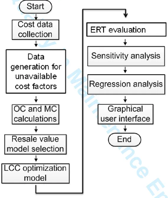
Figure 1 shows a flow chart of the LCC analysis used to meet the research goal.

Fig. 1. Flow chart for LCC analysis used in this study

Simply stated, the research described herein proposes an approach to LCC optimisation of the ventilation system used in Stockholm’s road tunnels based on calculations of the operating and maintenance cost, as well as purchase price and resale value. Note that we used a discount rate to account for the time value of money. To compare costs incurred at different times, it is necessary to shift expenditure to a reference point in time. Thus, we calculated the present equivalent value of the costs by considering the discount rate factor.

1 2 3 4 5 6 7 8 9 10 11 12 13 14 15 16 17 18 19 20 21 22 23 24 25 26 27 28 29 30 31 32 33 34 35 36 37 38 39 40 41 42 43 44 45 46 47 48 49 50 51 52 53 54 55 56 57 58 59 60

(6)

Journal of Quality in Maintenance Engineering

2.1 Data collection

Data were collected from MAXIMO, the database of Trafikverket’s CMMS. The study centred on two types of 121 fans installed in Stockholm’s road tunnels and drew on cost data for ten years (April 2005-December 2015).

The cost data in MAXIMO include corrective maintenance costs, preventive maintenance costs, and repair times. The corrective and preventive maintenance costs include spare parts and labour (repair person) costs. Operating costs, equipment purchase price, installation cost and other costs relevant to the case study were collected as well.It is important to mention that all cost data used in this study represent real costs without inflation. Because of company regulations, all cost data were encoded and expressed as currency units (cu).

Data are the only resource in a CMMS and are gathered from a variety of sources. If they are incorrect, incomplete, or inaccurate, the decisions based on them will be incorrect as well. MAXIMO includes basic modules to identify and codify assets, work orders, preventive maintenance and material events of equipment purchasing managers and warehouse management, as well as tools to analyse the information. These basic modules provide the foundation for an effective system of maintenance management. 2.2 Data quality problems

High quality information is dependent on the quality of the raw data and the way these data are processed. Data processing has shifted from providing operations support to becoming a major aspect of operations, making the need for quality data more urgent. Poor quality data result in customer dissatisfaction, lost revenue and higher costs associated with the additional time required to reconcile data. This can lead to a decline in a system’s credibility and increase the risk of noncompliance with regulations. It also increases consumer costs, increases taxes, decreases shareholder value, and may cause mission failure.

2.2.1 Incomplete data

The data in MAXIMO have many problems, mainly because of their manual input. Incomplete data is the main issue. Many fields contain null values, representing data neglected or forgotten by users. 2.2.2 Redundant data

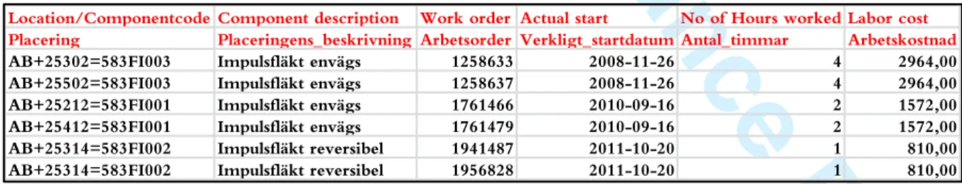
Redundancy is another issue. The same work order numbers often appear in several entries. This could result from bad communication or poor collaboration, causing the same work order to be entered by several different users. Table 1 shows an example.

Table 1. Redundant data

2.2.3 Inaccurate data

Accuracy is essential for good data quality. However, MAXIMO contains many inaccurate data; in thousands of fields, the value appears as zero, and this is clearly inaccurate.

2.3 Data generation for unavailable cost factors

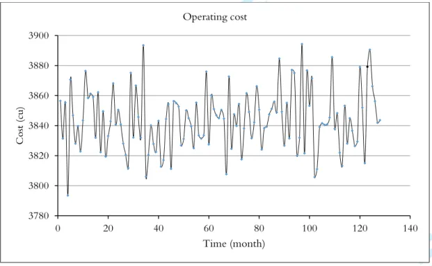
Operating cost data on the fans are generated each month, based on the energy price, the fans’ working hours, and the required power. Table 2 gives a sample of generated operating cost data from April 2005 to December 2015. The data were generated based on information from experts at Trafikverket involved in this study. The information they provided is the following:

Location/Componentcode Component description Work order Actual start No of Hours worked Labor cost Placering Placeringens_beskrivning Arbetsorder Verkligt_startdatum Antal_timmar Arbetskostnad AB+25302=583FI003 Impulsfläkt envägs 1258633 2008-11-26 4 2964,00 AB+25502=583FI003 Impulsfläkt envägs 1258637 2008-11-26 4 2964,00 AB+25212=583FI001 Impulsfläkt envägs 1761466 2010-09-16 2 1572,00 AB+25412=583FI001 Impulsfläkt envägs 1761479 2010-09-16 2 1572,00 AB+25314=583FI002 Impulsfläkt reversibel 1941487 2011-10-20 1 810,00 AB+25314=583FI002 Impulsfläkt reversibel 1956828 2011-10-20 1 810,00

1 2 3 4 5 6 7 8 9 10 11 12 13 14 15 16 17 18 19 20 21 22 23 24 25 26 27 28 29 30 31 32 33 34 35 36 37 38 39 40 41 42 43 44 45 46 47 48 49 50 51 52 53 54 55 56 57 58 59 60

(7)

Journal of Quality in Maintenance Engineering

• fans’ energy consumption: 25-80 kw/hour,

• fans’ operating time per day: 6-8 hours, • fixed energy price: 2.88 Swedish krona/kw.

Table 2. Sample of generated operating cost data

Figure 2 represents the data generated for the operating cost from April 2005 to December 2015

Fig. 2. Operating cost data 2.4 Operating and maintenance cost calculations

We calculated the maintenance costs (corrective and preventive) for each month of operation as follows:

3780 3800 3820 3840 3860 3880 3900 0 20 40 60 80 100 120 140 C os t ( cu) Time (month) Operating cost Page 6 of 18 Journal of Quality in Maintenance Engineering

1 2 3 4 5 6 7 8 9 10 11 12 13 14 15 16 17 18 19 20 21 22 23 24 25 26 27 28 29 30 31 32 33 34 35 36 37 38 39 40 41 42 43 44 45 46 47 48 49 50 51 52 53 54 55 56 57 58 59 60

(8)

Journal of Quality in Maintenance Engineering

MC

=

CM

+

PM

₍₁₎

c c CM =SP +LC

₍₂₎

p p PM =SP +LC

₍₃₎

We extrapolated the maintenance and operating costs to generate data for the unavailable period during the life cycle of the fans, as shown in Figures 3 and 4. As Trafikverket plans to use the fans for 20 years, we extrapolated operating and maintenance cost data for that length of time. Figures 3 and 4 illustrate the expected cumulative maintenance and operating costs determined by the data extrapolation for 121 fans as one system.

Fig. 3. Expected cumulative maintenance cost for 121 fans

Fig. 4. Expected cumulative operating cost for 121 fans

In Figures 3 and 4, the dots represent the real historical data for maintenance costs and the generated data for operating costs, respectively. We performed curve fitting using Table curve 2D software to show the behaviour of these costs after the time when data were collected. It is worth mentioning that fitting would be better if more data were available for a period longer than ten years. This software uses the least squares method to find a robust (maximum likelihood) optimisation for nonlinear fitting. As the figures show, the operating and maintenance costs increase over time. For example, the number of failures increases with time and the fans consume more energy because of degradation.

Expected CMC for 121 fans

0 60 120 180 240

Time (month)

0 5000 10000 15000 20000 25000 30000

C

ost

(c

u)

Expected COC for 121 fans

0 60 120 180 240

Time (month)

0 200000 400000 600000 800000 1000000

C

ost

(c

u)

1 2 3 4 5 6 7 8 9 10 11 12 13 14 15 16 17 18 19 20 21 22 23 24 25 26 27 28 29 30 31 32 33 34 35 36 37 38 39 40 41 42 43 44 45 46 47 48 49 50 51 52 53 54 55 56 57 58 59 60

(9)

Journal of Quality in Maintenance Engineering

2.5 Resale value model selection

We used a declining balance depreciation model to estimate the resale value of the fans after each month of operation. A fan’s resale value is its value if Trafikverket wants to sell it at any time during its planned lifetime. In this model, a fixed percentage of the book value at the beginning of the month represents the monthly depreciation of the ventilation system [8, 12, 13]. The resale value of the fans at time t, denoted as Rv(t), is given by the following formula [12]:

( )

1

(

1

)

t

Rv t =BV × −Dr

₍₄₎

where t represents time (month), t=1, 2, 3, …, 240, and BV1 is the book value on the first day of operation.

We modelled the depreciation rate that allows for full depreciation by the end of the planned lifetime (20 years) of the fans using the following formula [12]

:

1 1

1

L

SV

Dr

BV





= − 





_{ (5)}

where L represents the planned lifetime of the fans, i.e., 240 months.

The declining balance depreciation model is suitable in this case because it assumes more depreciation occurs at the beginning of an asset’s planned lifetime, less at the end. In accountancy, depreciation refers to two aspects of the same concept. The first is the decrease in an asset’s value; the second is the allocation of the cost of the asset to periods in which it is used. The scrap value is the estimate of the value of the asset at the time it is sold or disposed of. In this case study, 366 (cu) is assumed to be the scrap value of 121 fans at end of their planned lifetime, a figure given to us by experts at Trafikverket. Scrap value can be given as: PP SV L =

(6)

where PP represents the total initial cost (purchase price + installation cost) for all fans. In addition,

1

PP=PP TN×

₍₇₎

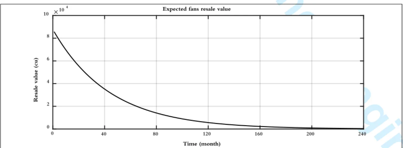
where PP1 represents the total initial cost for one fan and TN represents the total number of fans (i.e. 121)

Figure 5 shows the expected resale value using the declining balance depreciation model, as determined by MATLABTM_software.

Fig. 5. Expected resale value of fans

It is clear from Figure 5 that the resale value decreases with time until the fans reach scrap value at the end of their planned lifetime.

0 40 80 120 160 200 240 Time (month) 0 2 4 6 8 10

Resale value (cu)

104 Expected fans resale value

1 2 3 4 5 6 7 8 9 10 11 12 13 14 15 16 17 18 19 20 21 22 23 24 25 26 27 28 29 30 31 32 33 34 35 36 37 38 39 40 41 42 43 44 45 46 47 48 49 50 51 52 53 54 55 56 57 58 59 60

(10)

Journal of Quality in Maintenance Engineering

2.6 Total ownership cost model

The next step was to calculate the total ownership cost over each operating period. We defined the economic lifetime of the fans as the optimal age which minimises the total ownership cost. The total ownership cost over period i is denoted by TOCi, i= 1, 2, 3, ….,. By definition,

(

)

( )

1 RT i k k k TOC PP MC OC Rv t = = +



_

+



_

−



∑



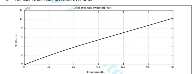
₍₈₎ where MCk and OCk are the maintenance and operating costs, respectively, for kth months.

We used total ownership cost because the fans’ PP, OC and MC represent costs, while the resale value represents income for Trafikverket when it is willing to sell the fans. Figure 6 illustrates the total expected ownership cost of the fans over the planned lifetime; we used MATLABTM_{software to calculate the total} ownership cost values.

As Figure 6 shows, the TOC increases with time for two reasons: 1. Operating and maintenance costs increase over time. 2. The fans’ resale value decreases over time.

Fig. 6. Total expected ownership cost 2.7 Life cycle optimisation model

We developed a life cycle optimisation model to estimate the economic replacement time of the fans comprising the ventilation system in Stockholm’s road tunnels. The objective was to determine the economic (optimal) replacement time to minimise the total ownership cost over all periods. We assumed the replacement fans would the same performance and cost as the old fans (i.e. identical fans). Therefore, the number of replacements during the optimisation time horizon is equal to:

Optimization time horizon Fans replacement time

T M RT =



_

 

_{ }

=



_









₍₉₎

where M represents the number of replacement cycles.

The economic replacement time is the value of RT that minimises the total ownership cost value, as shown in the following equation:

0 40 80 120 160 200 240 Time (month) 0 2 4 6 8 10 12 TOCi (cu)

105 Total expected ownership cost

1 2 3 4 5 6 7 8 9 10 11 12 13 14 15 16 17 18 19 20 21 22 23 24 25 26 27 28 29 30 31 32 33 34 35 36 37 38 39 40 41 42 43 44 45 46 47 48 49 50 51 52 53 54 55 56 57 58 59 60

(11)

Journal of Quality in Maintenance Engineering

(

)

( )

(

)

1 ₁ ₁₂ RT value i i i i M TOC PP MC OC Rv i r = = + + − × +     

∑



(10)

3. Results and discussion

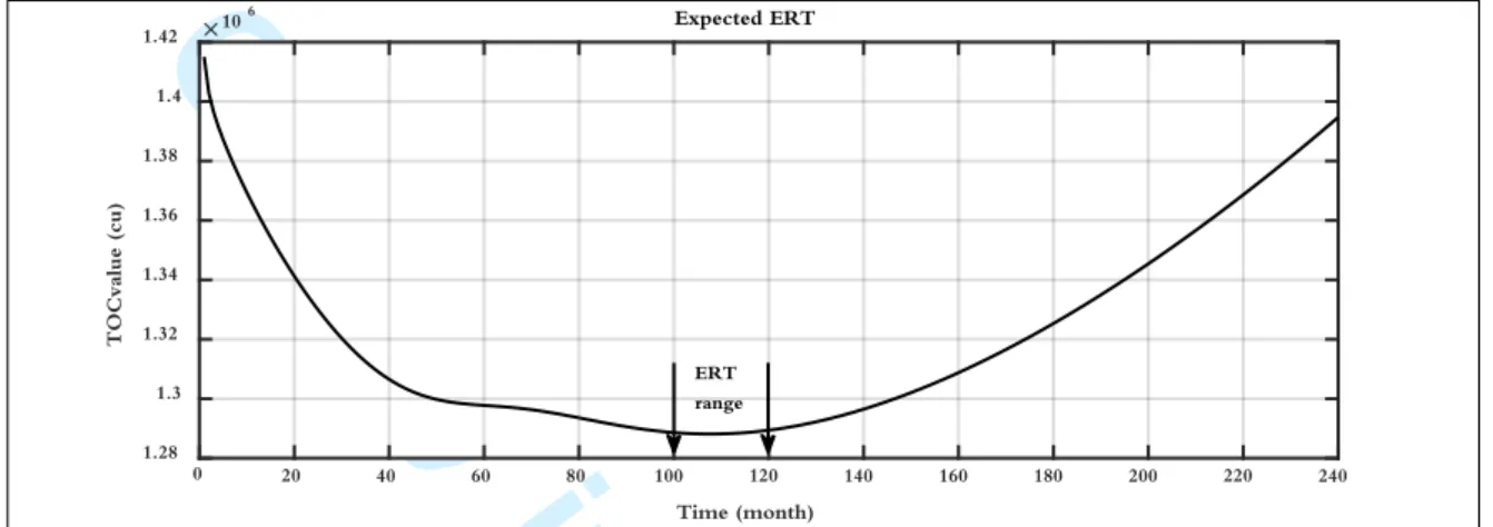
According to the results of the optimisation curve, the absolute ERT of 121 fans as one system is 108 months of operation. Figure 7 shows the results when we used MATLABTM_{software to obtain a variation} of the parameter RT of Eq. (10) for a period of 20 years (240 months).

Fig. 7. Economic replacement time of 121 fans as one system

Figure 7 also shows a range 100-120 months when the minimum TOC value can still be achieved in practice. In our terminology, this is the economic replacement time range. Finding the economic replacement time range is an important result of our study as it can help users (in this case Trafikverket) in their planning. Trafikverket has the flexibility to make replacements within the economic replacement time range of 20 months. There is no fixed date or age within this range at which the total cost is at a minimum, but a decision to replace the system before or after this economic replacement time range will incur greater costs. The use of a lower replacement age (i.e. less than 100 months) will incur higher costs because of the high investment cost. Meanwhile, if the lifetime of the system exceeds the upper limit of this range, losses will increase for two reasons:

1. The cost of operation and maintenance increases when the operating time increases because of fan degradation.

2.

A fan’s resale value will decrease each month of operation until it reaches its scrap value at the end of its planned lifetime (i.e. 240 months).

3.1 Sensitivity analysis

We performed sensitivity analysis to identify the effect of purchase price and operating and maintenance costs on the economic age of replacement. Since most of the factors were likely interrelated, we used multi-sensitivity analysis to identify the effect of multiple changes in cost factors.

3.1.1 Single-variable sensitivity analysis

Single-variable sensitivity analysis varies one factor and keeps the others constant. In our sensitivity analysis, we included the system purchase price and the operating and maintenance costs. Figure 8 illustrates the effect of an increasing purchase price on the ERT of the fans comprising the ventilation system.

Figure 8 shows the ERT is an increasing step function of PP (based on the percentage of purchase price); the ERT remains constant for a specific range of PP increments, then increases stepwise. As an example, if the purchase price increases by 1% to 3%, the ERT is constant. This means the ERT increases stepwise at specific PP percentage increments, i.e. 1, 3, 4, 5, 6, 8, 9, 11, 12, 13, 15, 16, 18, 19, 21, 22, 24, 26, 27, 29, 31, 32, 34, 36, 38, 39, 41, 43, 45, 47 and 49%. In other words, the system purchase price has a major effect on the ERT.

0 20 40 60 80 100 120 140 160 180 200 220 240 Time (month) 1.28 1.3 1.32 1.34 1.36 1.38 1.4 1.42 TOCvalue (cu) 106 Expected ERT ERT range Page 10 of 18 Journal of Quality in Maintenance Engineering

1 2 3 4 5 6 7 8 9 10 11 12 13 14 15 16 17 18 19 20 21 22 23 24 25 26 27 28 29 30 31 32 33 34 35 36 37 38 39 40 41 42 43 44 45 46 47 48 49 50 51 52 53 54 55 56 57 58 59 60

(12)

Journal of Quality in Maintenance Engineering

Fig. 8. Effect of increasing purchase price

Figure 9 illustrates the effect of decreasing operating cost (based on the percentage of operating cost) on the ERT. It is obvious that when the system’s operating cost decreases, the ERT increases linearly, although it remains constant within a specific range of decreasing OC. This means the ERT is not sensitive to a specific percentages of operating cost reductions, i.e. 2, 7, 12 and 18%. The system’s ERT will increase linearly at 46 out of 50 percentages of OC reduction. Thus, the system’s operating cost has the biggest effect on its ERT.

Fig. 9. Effect of decreasing operating cost

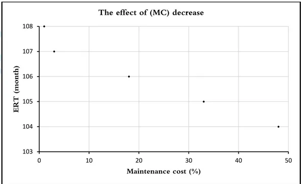
Figure 10 illustrates the effect of decreasing the maintenance costs on the ventilation system’s ERT. When the maintenance cost decreases, the ERT decreases as a step function of MC reduction. In addition, the ERT decreases in the various MC reduction percentages, i.e. 3, 18, 33, and 48%, but remains constant within these percentages. This means the ventilation system’s ERT is not sensitive to maintenance cost reductions. 100 110 120 130 140 0 10 20 30 40 50 ER T ( m onth ) Purchase price (%)

The effect of (PP) increase

100 120 140 160 0 10 20 30 40 50 ER T ( m onth ) Operating cost (%)

The effect of (OC) decrease

1 2 3 4 5 6 7 8 9 10 11 12 13 14 15 16 17 18 19 20 21 22 23 24 25 26 27 28 29 30 31 32 33 34 35 36 37 38 39 40 41 42 43 44 45 46 47 48 49 50 51 52 53 54 55 56 57 58 59 60

(13)

Journal of Quality in Maintenance Engineering

Fig. 10. Effect of decreasing maintenance cost 3.1.2 Multi-variable sensitivity analysis

To increase our understanding of the correlation of input and output variables in the optimisation model, we performed multi-sensitivity analysis, considering three different cases. More specifically, MATLABTM software allowed us to vary three variables, increasing factor of purchase price (IFPP), reduction factor of maintenance cost (RFMC), and reduction factor of operating cost (RFOC) to show their effects on the ERT of the ventilation system. In all three cases, the purchase price increased while the operating and maintenance costs decreased.

Fig. 11. Effect of RFOC, IFPP and RFMC on the ERT of the ventilation system

Case one considered the effect of decreasing the fans’ operating cost (1%-50%) while increasing the purchase price at (3, 9, 16, 24, 32, 41 and 49%) at a given maintenance cost decrease of 3%. As Figure 11 shows, decreasing the operating cost while increasing the purchase price has a positive effect on increasing the system’s economic replacement time.

Case two considered the effect of increasing the purchase price (1%-50%), while decreasing the operating cost at different percentages (3, 11, 20, 27, 34, 41 and 48%) and, at the same time, decreasing maintenance

103 104 105 106 107 108 0 10 20 30 40 50 ER T ( m onth ) Maintenance cost (%)

The effect of (MC) decrease

100

110

120

130

140

150

160

170

180

190

0 5 10 15 20 25 30 35 40 45 50

E

R

T

(

mont

h)

OC decrease (%)

Effect of RFOC, IFPP for given 3% RFMC

pp 3%,

pp 9%

pp 16%

pp 24%

pp 32%

pp 41%

pp 49%

1 2 3 4 5 6 7 8 9 10 11 12 13 14 15 16 17 18 19 20 21 22 23 24 25 26 27 28 29 30 31 32 33 34 35 36 37 38 39 40 41 42 43 44 45 46 47 48 49 50 51 52 53 54 55 56 57 58 59 60

(14)

Journal of Quality in Maintenance Engineering

costs by 3%. As Figure 12 shows, increasing the purchase price while decreasing the operating cost has a

positive effect on increasing the system’s economic replacement time.

It is obvious from Figures 11 and 12 that the effect on the ERT of decreasing the operating cost is more than the effect of increasing the purchase price.

Fig. 12. Effect of IFPP, RFOC, and RFMC on the ERT of the ventilation system

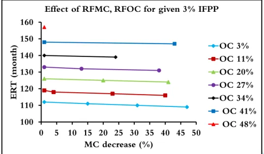
Finally, case three considered the effect of decreasing the maintenance cost (1%-50%) while decreasing the operating cost at different percentages (3, 11, 20, 27, 34, 41 and 48%) and increasing the purchase price by 3% at the same time. As Figure 13 shows, there is a very small effect on the ERT when the maintenance cost is decreased and there is a positive effect on the ERT when the operation cost is reduced.

Fig. 13. Effect of RFMC, RFOC and IFPP on the ERT of the ventilation system

In general, the results of the sensitivity analysis indicated that increasing the purchase price and decreasing the operating costs both have a positive effect on increasing the ERT, but the effect of decreasing the maintenance cost is too small to be of significance.

3.2 Regression analysis

For our regression analysis of the results obtained from three MATLAB codes for the previous three cases, we used Minitab software and the least squares method. We modelled economic replacement time as a linear function of IFPP, RFOC and RFMC. IFPP is the percentage increment on the system’s purchase price, RFOC is the percentage reduction in the system’s operating cost, and RFMC is the percentage

100 110 120 130 140 150 160 170 180 190 0 5 10 15 20 25 30 35 40 45 50 E R T ( mont h) PP increase (%)

Effect of IFPP, RFOC for given 3% RFMC

OC=3% OC=11% OC=20% OC=27% OC=34% OC=41% OC=48%

100

110

120

130

140

150

160

0 5 10 15 20 25 30 35 40 45 50

E

R

T

(

mont

h)

MC decrease (%)

Effect of RFMC, RFOC for given 3% IFPP

OC 3%

OC 11%

OC 20%

OC 27%

OC 34%

OC 41%

OC 48%

1 2 3 4 5 6 7 8 9 10 11 12 13 14 15 16 17 18 19 20 21 22 23 24 25 26 27 28 29 30 31 32 33 34 35 36 37 38 39 40 41 42 43 44 45 46 47 48 49 50 51 52 53 54 55 56 57 58 59 60

(15)

Journal of Quality in Maintenance Engineering

reduction in the system’s maintenance cost. The regression analysis resulted in the following mathematical

model:

104,229 0,652 0,012 1,032

ERT = + IFPP− RFMC+ RFOC

₍₁₁₎

where IFPP = 5%, RFMC = 3%, and RFOC = 11%. The ERT can be calculated by the regression model as follows:

104.229 0.652 5 0.012 3 1.032 11 118.8 119 ( )

ERT = + × − × + × = ≈ month

The ERT obtained from the regression model is compatible with the values shown in Figure 12. The other values of IFPP, RFMC and RFOC can be calculated and checked as well.

The high R-squared adjusted value obtained from regression analysis, 99.16, indicates that the ERT of the new system depends linearly on the variables of PP, OC and MC. Following the results of the sensitivity and regression analyses, the parameters affecting the increase in the ERT are the following:

1. operating cost of the system; 2. purchase price of the system; and 3. maintenance cost of the system.

The results of the regression analysis show that the operating cost has the largest impact on the ERT, followed by the purchase price and the maintenance cost; therefore, the manufacturer should focus on improving the reliability and maintainability of the fans to reduce the costs associated with operating and maintenance and to increase their ERT.

3.3 Graphical user interface

During the study, we discovered Trafikverket cannot always use the process introduced here. Therefore, to facilitate decision making and enhance Trafikverket’s ability to make the right decision at the right time, we developed a graphical user interface to compute the ERT of the ventilation system. The personnel in the Trafikverket financial department and/or maintenance department can easily use the graphical user interface to estimate the ERT of new fans and determine their ERT behaviour for different values of IFPP, RFOC and RFMC. These factors will give a clear view of the ERT of new fans, helping Trafikverket determine when to buy a new asset and assisting the company in any negotiations with the manufacturer on the purchase price of new models. Figure 14 represents the GUI for case one (operating cost).

The selected input factors appear on the left side of the figure; the program calculates the ERT of a new ventilation system based on the selected input. The generated fields shown on the right of the figure represent the ERT values, calculated after applying the proposed optimisation model. A plot representing the ERT trend appears in the central column. From this, decision makers can determine the best time economically to buy a new ventilation system. After choosing one of three factors, purchase price, operating cost, or maintenance cost, they can determine its effect on the ERT by plotting it in the interface.

Fig. 14. Graphical user interface for the operating cost

1 2 3 4 5 6 7 8 9 10 11 12 13 14 15 16 17 18 19 20 21 22 23 24 25 26 27 28 29 30 31 32 33 34 35 36 37 38 39 40 41 42 43 44 45 46 47 48 49 50 51 52 53 54 55 56 57 58 59 60

(16)

Journal of Quality in Maintenance Engineering

3.4 Data quality results

The results show data quality (DQ) problems have direct impacts on the information generated from those data. For example, costs are affected by different types of dirty data, such as redundant, incomplete or inaccurate data. Maintenance decisions will also be affected, leading to wrong or delayed decisions. 3.4.1 Impact on data analysis

The collected data were dirty, with a direct impact on the cost analysis generated from those data. For example, Figure 15 shows the number of fans before data cleaning to be 122, but after data cleaning, we see 121.

Fig. 15. Number of fans

The number of failures is also affected by bad data. Figure 16 shows the number of failures is reduced after data are cleaned. The number before cleaning is 1414 and the number after cleaning is 662.

Fig. 16. Number of failures

Figure 17 gives the number of failures and number of fans for each type of fan before data cleaning, and Figure 18 gives the same information after data cleaning. As the two figures clearly tell us, data cleaning matters. Dirty data will have a negative impact on the LCC estimation, the maintenance cost estimation, and the economic replacement time estimation of the ventilation system.

120 121 122 1 2 122 121 N o. of f ans

Before data cleaning - After data cleaning

Ventilation system 0 200 400 600 800 1000 1200 1400 1600 1 2 1414 662 N o . o f fa ilu re s

Before data cleaning - After data cleaning

Ventilation system

1 2 3 4 5 6 7 8 9 10 11 12 13 14 15 16 17 18 19 20 21 22 23 24 25 26 27 28 29 30 31 32 33 34 35 36 37 38 39 40 41 42 43 44 45 46 47 48 49 50 51 52 53 54 55 56 57 58 59 60

(17)

Journal of Quality in Maintenance Engineering

Fig. 17. Number of failures and number of fans for each type of fan before data cleaning

Fig. 18. Number of failures and number of fans for each type of fan after data cleaning 4. Conclusions

Based on the results, we developed the following conclusions:

1. This study proposes a practical approach to determining the economic replacement time of a ventilation system used in Stockholm’s road tunnels. Although many other models require reliability and failure data to identify the optimum replacement age, the approach presented herein is based on financial data on the purchase price, operating and maintenance costs, and the system’s resale value. This makes it very practical for Trafikverket.

2. According to the results obtained from the optimisation curve, the absolute ERT of the ventilation system is 108 months of operation. However, the ERT has a range of 100 to 120 months, during which the total ownership cost remains almost constant. There is no single fixed date or age at which the TOC value is minimum. This gives Trafikverket the flexibility to make replacements within an optimum replacement age range of 20 months. Finding the economic replacement age range is an important result of our study, given its ability to help Trafikverket in its planning.

3. The results of the sensitivity analysis to identify the effect of various factors on the economic replacement time indicate that increasing the purchase price and decreasing the operating cost

0 30 60 90 120 150 180 1 3 5 7 9 11 13 15 17 19 21 23 25 27 29 31 29 172 44 61 37 22 26 18 85 21 72 58 41 23 40 253626 68 26 68 56 124 5065 13 3 63 15 16 11 2 3 4 4 5 4 4 3 6 6 4 3 5 5 3 3 5 3 4 4 4 6 8 4 5 4 1 4 2 2 2 N o . o f fa ilu re s Fan type

Failures analysis for 10 years

No. Of failures No. Of fans

0 20 40 60 80 100 120 1 3 5 7 9 11 13 15 17 19 21 23 25 27 29 31 13 105 172021 9 1117 32 20 35 26 151618112013 28 1321 29 57 1524₁₀ 1 23 10 4 8 2 3 4 4 5 4 4 3 6 6 4 3 5 5 3 3 5 3 4 4 4 6 8 4 5 3 1 4 2 2 2 N o . o f fa ilu re s Fan type

Failures analysis for 10 years

No. Of failures No. Of fans

1 2 3 4 5 6 7 8 9 10 11 12 13 14 15 16 17 18 19 20 21 22 23 24 25 26 27 28 29 30 31 32 33 34 35 36 37 38 39 40 41 42 43 44 45 46 47 48 49 50 51 52 53 54 55 56 57 58 59 60

(18)

Journal of Quality in Maintenance Engineering

have a positive effect on increasing the system’s ERT, but decreasing the maintenance cost has a

small effect.

4. The results of the regression analysis using three factors (IFPP, RFOC and RFMC) show that the ERT of the new ventilation system depends linearly on its IFPP, RFOC and RFMC. These results confirm the computation and the results of the sensitivity analysis.

5. The results of regression analysis also show that the operating cost has the largest impact on the ERT, followed by the purchase price and maintenance cost. Hence, the manufacturer must make a greater effort to improve the reliability and maintainability of the fans to reduce the costs associated with operation and maintenance and to increase their ERT.

6. Economists and maintenance managers at Trafikverket can easily use the GUI to estimate the ERT of a new system and anticipate the behaviour of its ERT at IFPP, RFOC and RFMC. These factors will provide a clear view of the ERT of the new system, helping Trafikverket to determine when to buy a new system and assisting it in negotiations with the manufacturer over the purchase price.

7. Data quality problems have a direct impact on LCC analysis and maintenance efficiency. The LCC analysis and maintenance management activities based on MAXIMO data are likely to be affected by the poor quality of those data. For example, the costs of maintenance could change after data are cleaned. Therefore, the data quality of MAXIMO needs to be improved.

8. The main reason for data quality problems is the manual input of MAXIMO data. Manual input is always subjective. Missing, redundant, or inaccurate data are generated by human errors. The data collection needs to be automated, especially with the revolution in Information and Communication Technology (ICT), including cloud computing and the Internet of Things (IoT). The use of ICT tools can ensure high quality data, improve maintenance efficiency, and enhance decision making.

9. Information can be considered an item, and data are its raw material. Since the nature of the item must be in the same class as the nature of its raw materials, Trafikverket must put resources into information quality. It could begin with constrained data profiling and information purifying exercises; this could quickly develop into a powerful information quality assurance program. Acknowledgments

The research was carried out in 2016 at the Division of Operation, Maintenance and Acoustics, Luleå University of Technology, Sweden. The research program was sponsored by the Swedish Transport Administration (Trafikverket).

The support of Trafikverket during the research is deeply appreciated, especially the help of Thomas Rolén, and Kerstin Abrahamsson.

I would like to express my sincere gratitude to Peter Söderholm for his invaluable guidance, suggestions and support. Karim, Hawzheen, Stefan Jonsson and Lars Schillström are also gratefully acknowledged. References

[1] Jardine A, Tsang A. Maintenance, Replacement, and Reliability Theory and Application. New York: Taylor & Francis Group; 2006.

[2] Farr JV. Systems Life Cycle Costing: Economic Analysis, Estimation, and Management. New York: CRC Press; 2011.

[3] Norton RL. Machine Design: an Integrated Approach. 4th ed. Upper Saddle River, N.J: Pearson; 2011.

[4] Ryan W. Procurement views of life cycle costing. In: Proceedings of the 1968 Annual Symposium on Reliability, Boston, Massachusetts 1968 January 16-18; 164-168.

[5] Seldon MR. Life Cycle Costing: a Better Method of Government Procurement. Westview Press: Boulder, Colo; 1979.

[6] Brown RJ. A new marketing tool: life-cycle costing. Industrial Marketing Management 1979; 8(2), 109-113.

[7] Earles ME. Factors, Formulas and Structures for Life Cycle Costing. Eddins-Earles, Concord, Mass; 1981.

[8] Dhillon BS. Life Cycle Costing for Engineers. New York: CRC Press; 2010.

1 2 3 4 5 6 7 8 9 10 11 12 13 14 15 16 17 18 19 20 21 22 23 24 25 26 27 28 29 30 31 32 33 34 35 36 37 38 39 40 41 42 43 44 45 46 47 48 49 50 51 52 53 54 55 56 57 58 59 60

(19)

Journal of Quality in Maintenance Engineering

[9] Dhillon BS. Design Reliability: Fundamentals and Applications. New York: CRC Press; 1999.

[10] Al-Chalabi H, Lundberg J, Ahmadi A, Jonsson A. Case Study: Model for economic lifetime of drilling machines in the Swedish mining industry. The Engineering Economist 2015; 60(2): 138-154. [11] Al-Chalabi H. S, Lundberg J, Al-Gburi M, Ahmadi A, Ghodrati B. Model for economic replacement time of mining production rigs including redundant rig costs. Journal of Quality in Maintenance Engineering 2015; 21(2): 207-226.

[12] Luderer B, Nollau V, Vetters K. Mathematical Formulas for Economists. 4th ed. New York: Springer Heidelberg Dordrecht; 2010.

[13] Eschenbach T. Engineering Economy: Applying Theory to Practice. 3rd ed. New York: Oxford University Press; 2010.

1 2 3 4 5 6 7 8 9 10 11 12 13 14 15 16 17 18 19 20 21 22 23 24 25 26 27 28 29 30 31 32 33 34 35 36 37 38 39 40 41 42 43 44 45 46 47 48 49 50 51 52 53 54 55 56 57 58 59 60