Stable and Unstable Debt Dynamics : Does Debt Monetizing Policy Matter?

J

I

B

S

JÖNKÖPING UNIVERSITY

Stable and Unstable Debt

Dynamics

Does Debt Monetizing Policy Matter?

Bachelor Thesis within Economics Author: Yuliya Bilinskaya

Tutor: Associate Professor Martin Andersson Ph.D Candidate Dimitris Soudis Date: June 2010, Jönköping

i

Bachelor Thesis within Economics

Title: Stable and Unstable Debt Dynamics. Does Debt Monetizing Poli-cy Matter?

Author: Yuliya Bilinskaya

Tutors: Martin Andersson, Associate Professor Dimitris Soudis, Ph.D Candidate

Date: 2010-06-03

Keywords: Stable/Unstable Debt Dynamics, Monetizing Policy, Bond Is-suance Policy, Budget Balance, Government Debt

Abstract

This thesis analyzes the effect of the two Debt Financing policies: Monetary and Bond Issuing, on the Dynamics Development. Economic variables, like GDP growth, interest rate and inflation are discussed, as the key determinants in the Debt Dynamics process development. The proposition of countries EMU members having higher Debt Dynam-ics level is suggested. This proposition is based on the fact that EMU member countries cannot use their Monetary policy to the extend it is needed in hard times. Due to this lack of choice EMU members can only intensively use Bond financing. The empirical findings of the paper indicate that the difference in Debt Dynamics between the euro us-ing and non-usus-ing countries exists. The difference indicates that the EMU member countries tend to have higher Debt Dynamics than the rest of the EU countries. These findings are discussed from different sides, concluding that Monetary Policy does mat-ter in certain cases. At the same time a quite high level of Debt Dynamics in both groups is discovered, which is also an interesting issue to address.

ii

Table of Contents

Abstract ... i

Tables ... iii

Figures ... iii

1

Introduction ... 1

1.1 Research problem and purpose ... 2

1.2 Historical overview of the Last Decades ... 2

1.2 Outline ... 5

2

Budget Deficits, Government Debts, and Debt

Dynamics Theoretical Framework ... 6

2.1 Budget Deficit Definition and Debt Accumulation ... 6

2.2 Debt Dynamics ... 6

2.2.1 Stable Debt Dynamics ... 7

2.2.2 Unstable Debt Dynamics ... 8

2.3 Bond Financing ... 9

2.4 Monetary Policy ... 10

2.5 EMU and ECB ... 11

3

Statistical Methods and Results ... 13

3.1 Data Analysis and Hypothesis ... 13

3.2 Panel Least Squares Analysis ... 13

3.3 Regression Results ... 14

4

Analysis ... 16

5

Conclusions ... 18

5.1 Suggestion for Further Research ... 18

6

References ... 19

6.1 Scientific Publications ... 19

6.2 Websites ... 20

iii

Tables

Table 1: Government Debt as % of GDP ... 1 Table 2: Regression results of Panel Least Squares: Variables, Coefficients and

Significance Levels ... 14 Table 4: EU countries’ currency use and exchange rate regimes ... 22

Figures

Figure 1: Some EU countries, Exceeding the Threshold Level ... 3 Figure 2: Comparison of Some EU Countries’ Debt Levels ... 4 Figure 3: EU (EA11-2000, EA12-2006, EA13-2007, EA15-2008, EA16) Annual GDP

growth, Short Term Interest Rate (12 months) and Long Term Interest Rate (10 years Government Bond) ... 5 Figure 4: Stable Debt Dynamics ... 8 Figure 5: Unstable Debt Dynamics ... 8 Figure 6: European Monetary Union Institutional Structure and the Role of European

1

1 Introduction

The Debt level, counted in trillions of euro is no more something extraordinary. In 2009, European Union (EU) countries like Germany, France, United Kingdom and Ita-ly have passed a 1 trillion euro Debt level (Eurostat). The situation does not change dramatically if we look at what portion of GDP of these countries is financed by Debt, as shown in the Table 1.

Table 1: Government Debt as % of GDP

Country Debt as % of GDP United Kingdom 68,1 Germany 73,2 France 77,6 Italy 115,8 Source: Eurostat

The disturbing factor in the Debt trend is its steady increase over the past decade. In some cases, the Debt level has been increasing at such high levels, that the need for ac-tive measures is becoming necessary. OECD Economic Outlook for the end of 2009 has made the projections of the Debt levels rising even further in most of the countries at least until the end of 2011. This prognosis makes the topic actual for the coming years, as the paying back and stabilization period will take considerable amount of time. The reasons for the Government Debt Dynamics increasing every year are: running Budget Deficits, Snowball Effect; or the mixture of the two reasons (Isaac, 2009; Report of the Swedish Fiscal Policy Council, 2010).

The first term, Budget Deficit, occurs when the government is spending more than it earns and can be adjusted directly by the fiscal policy (The Economist, Dictionary). Nevertheless, even turning budget deficits into surpluses or at least reducing them to ze-ro level are not easy tasks to do. First of all this will require political agreement among policy makers to implement long-term strategies, which is the only way to reduce the debt, accumulated over decades. Secondly, deficit reductions are often accompanied by unpopular fiscal policies like tax increase or transfer reductions, especially in the short-run. Such measures can cause dissatisfaction among population and fall of the populari-ty of the ruling government, which can be a deep concern of many politicians (Shojai, 1999).

The second term Snowball Effect is a trend in the increasing Debt occurring due to the processes, imbedded into the Debt Dynamics equation. In other words, Snowball Effect indicates by how much the level of debt would be increasing, even if the country would have a zero Budget Deficit. This is a more complex process, involving economic indica-tors like short-term interest rate, GDP growth rate and inflation. The difference between these variables makes the Debt Dynamics to be Stable or Unstable. Nevertheless, Snowball Effect can be influenced by the policy, the government chooses to finance the debt with.

In case of Bond Issuance policy, large debt levels in well-developed countries cause crowding out of investments and consequently reduce growth (Argimon &

Gonzalez-2

Paramo & Roldan, 1997). Another possible process is the Barro-Ricardo equivalence, suggesting that the government’s attempts to stimulate private expenditures through tax cuts will not be successful.

Monetary policy is another tool to finance the government Debt. In this case, the gov-ernment is Monetizing the Debt, which is an attempt to gain the seignorage from the money printing until a certain level, when the costs of higher inflation start surpassing the seignorage (Fischer & Easterly, 1990). Another reason for this policy is the govern-ment’s effort to inflate the accumulated stock of Debt by reducing its real value (Vieira, 2000). The country will automatically experience the depreciation/devaluation of its currency, damaging the Trade Balance (Fischer & Easterly, 1990). The situation will stabilize itself after some period, when the depreciated/devalued currency will attract the investments from the rest of the world, improving the Trade Balance.

Consideration of European Union countries, raises an interesting question about the lev-el of the Debt Dynamics when the country does not have a choice of Debt Financing strategy. This is the case of the European Monetary Union (EMU) countries, whose supply of money is entirely controlled by European Central Bank (ECB). Therefore, these countries are left only with the Bond Issuance policy. Can this fact lead to higher Debt levels through increased Snowball Effect in these countries?

1.1 Research problem and purpose

This paper will link the two important aspects of Macroeconomic theories: Debt Financ-ing Policies and Debt Dynamics process development. Today’s research in the field of Debt Financing is mainly looking at the Debt accumulation due to the Budget Deficit running. In contrast, this thesis is looking at how these Bond Issuance and Monetary policies can affect the Snowball Effect and consequently the Debt level if used solely. It is worth underlining, that the reasons of Debt increase due to the Budget Deficit running will not be the main focus, even so Budget Balance is controlled for in the regression. Further, I will analyze if the inability to use Monetary Policy to finance the Debt can lead to higher Debt Dynamics, compared to the countries, which are able to use both strategies. For this thesis Dated Panel Least Squares method with fixed effects was cho-sen including information for all EU countries for the period 1996-2009.

The purpose of this thesis is to analyze whether the countries-members of European Monetary Union have higher level of Debt Dynamics, or leaning towards Unstable Debt Dynamics, compared to the rest of the countries in the European Union. An overview of the major consequences of Bond Financing and Debt Monetizing strategies will be giv-en, focusing on interest rates, GDP growth and inflation. These strategies’ possible ef-fect on the Debt Dynamics process development will be discussed.

1.2 Historical overview of the Last Decades

Many economists conclude that the alarming steady increase of countries’ Debt levels is an underestimated problem of the present and can cause serious effects in the nearest fu-ture. There are two main principles of the Stability and Growth Pact (SGP) of the EU. The first one states that the deficit level must not exceed 3% of GDP. The second prin-ciple is that the country’s debt level must not exceed 60% of GDP (Government Finance Statistics, Eurostat Yearbook 2009). Revision of the Pact in 2005 allowed for

3

higher deficit and debt levels as an exception in hard economic times, but left the rules unchanged.

Before 1970s, countries were mostly influenced by Keynes’ theories on functional finance and smoothing out the cyclical effects of the economy. The main goal was to make budget surplus during peace times and allowing for budget deficit, by spending increase, during wars or other disturbances (Shojai, 1999). This way the governments were trying to achieve zero accumulated debt over the long run.

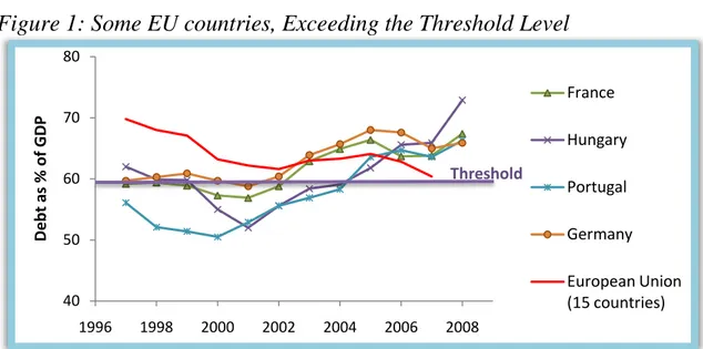
Nevertheless, Figure 1 shows a range of countries, which have been violating SGP rules even during peace times. Even the overall level of EU countries’ Debt represented by the European Union (15 countries) line has been constantly above the threshold level.

Figure 1: Some EU countries, Exceeding the Threshold Level

Source: Eurostat

A rough look at the Figure 1 shows a steady trend of Debt increase since year 2000 in this group of countries. We can see that these countries could not stop the Debt growth even after they crossed the threshold level of 60%. The latest research shows that when Gross External Debt reaches 60% of GDP, annual growth rate declines by about 2 % of the previous year’s growth; for levels higher than 90% of GDP, growth rates are rough-ly cut in half (Reinhart & Rogoff, 2010). This may not have a great impact on GDP in the short run, but the situation changes if the country is keeping its high level of debt over the long run. As seen from the Figure 1 and Figure 2, this can surely be the case of some EU countries.

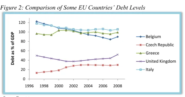
Figure 2 gives the comparison between the extreme cases of Debt increase, such as Greece, Belgium and Italy, which have clearly exceeded a 100% level over the past decade, and the countries with lower level of Debt increase.

40 50 60 70 80 1996 1998 2000 2002 2004 2006 2008 De bt a s % of GDP France Hungary Portugal Germany European Union (15 countries) Threshold

4

Figure 2: Comparison of Some EU Countries’ Debt Levels

Source: Eurostat

As we can see, the countries can have the debt levels change at different magnitudes. For example, Czech Republic has been roughly within the 15-30% band, UK 40-60% and Italy 120-100%. Nevertheless, this fact does not necessary mean, that Belgium is having more difficulties with managing its Debt than for example UK. This suggestion is based on the fact that all countries have different Debt Intolerance levels, meaning that a country can default even if its Debt level is comparatively low. The level of Debt Intolerance depends heavily on the country’s previous records of default and inflation (Reinhart & Rogoff & Savastano, 2003). This proposition implies, that for our analysis all countries will be considered, not depending on their Debt levels.

As mentioned before, the development of Government Debt can be caused by: Budget Deficits and the Snowball Effect. For that reason, I will briefly show the trends of both processes over the last decades.

The common definition explains that government debt is an accumulated level of budg-et deficits over time (The Economist, Dictionary). Historical underlying reasons of high debt trends are the expenditure and revenue levels in the Budget Balance of some EU countries. Rapid deficit increase since 1960s, is explained by revenue and expenditure imbalances, both of which grew over time, but expenditures had a significantly larger increase (Shojai, 1999). On average, there has been a dramatic jump from 24% of gov-ernment expenditures in 1960 to 50% in 1990 (Shojai, 1999). For example, Denmark and Finland increased up to 56% level of government expenditures, when France and Norway became 50% (OECD Statistics).

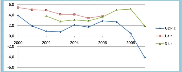
The second reason, which is the Snowball effect1, is dependent on the relation between the short-term interest rates and the GDP growth. The effect arises when these two va-riables are close to each other in values, leading to Stable Debt Dynamics; and becomes severe, when the interest rate exceeds the growth rate, leading to Unstable Debt Dynam-ics. As shown in Figure 3, the Unstable Debt Dynamics is very strong in some of the EU countries, resulting in the high interest rates and low growth. We should keep in

1 _{Detailed explanation of the effect and its underlying reasons will be explained in Section 2.2}

0 20 40 60 80 100 120 1996 1998 2000 2002 2004 2006 2008 D ebt as % o f GD P Belgium Czech Republic Greece United Kingdom Italy

5

mind that Figure 3 shows the overall relation of EU countries, meaning that there can be significant differences in the Debt Dynamic levels between the countries. As we can al-so see, the latest financial crisis has enlarged the gap between the interest rate and the GDP growth even more.

Figure 3: EU (EA11-2000, EA12-2006, EA13-2007, EA15-2008, EA16)

Annual GDP growth, Short Term Interest Rate (12 months) and Long Term

Interest Rate (10 years Government Bond)

Source: Eurostat

As we have seen, both reasons for increasing debt have been present in the past decade. High imbalances in the budget deficits of some countries were due to the increasing ex-penditures and the political structure of the government. Weak and divided governments (divided in terms of number of parties present in the ruling power) were clearly less successful in reducing the government debt (Roubini & Sachs, 1988).Some countries even during peacetime kept on running deficits and accumulating debt, indicating the shift from the Keynes’ theories on functional finance. The other term, the Snowball ef-fect has also been present in a range of EU countries, but has been paid much less atten-tion to. Moreover, this process needs clear stabilizaatten-tion policies. Otherwise, in case the Snowball effect leads to Unstable Dynamics, the country will eventually default.

1.2 Outline

Section 2 gives theoretical framework on the Monetary and Bond Issuance policies as well as linking their influence to the theory on Debt Dynamics. The derivations of Debt Dynamics equation is presented with the explanation of two cases: Stable and Unstable Debt Dynamics. Section 3 introduces the empirical methods and results of the per-formed analysis. Further, Section 4 analyzes the empirical findings from the regression and links them to the theoretical framework. Finally, Section 5 concludes the paper.

-6,0 -4,0 -2,0 0,0 2,0 4,0 6,0 2000 2002 2004 2006 2008 GDP g L-t r S-t r

6

2 Budget Deficits, Government Debts, and Debt Dynamics

Theoretical Framework

2.1

Budget Deficit Definition and Debt Accumulation

First of all, Budget Deficit is defined by the following formula:

t t

p

t

G

Tx

Tr

D

(

)

(1)

where Dpt2 is the primary deficit, Gt is government spending, Tx is tax collections and

Tr is the transfers. Gt represents the expenditure level of the government, while (Tx –

Tr)t represent the revenues. Therefore, Budget Deficit occurs when government

spend-ing is higher than government revenue in the current period.

Economic theory identifies two types of Budget Deficits: cyclical and structural. Cyc-lical Deficits are related to the fall in the government revenue (fall in tax collections in particular), when the economy is experiencing a downturn. In this case, if the govern-ment reduces expenditures in order to eliminate budget deficit, the economy will wea-ken even further. Nevertheless, as the situation is short-term, budget deficit will come up to zero once the economy is back to full production.

Structural Deficits are not connected to the fluctuations in the economy and occur when the output is at its maximum level. They arise due to the government’s intentional deci-sion to spend more than it gets through tax collections. Structural Deficits are the ones that over the long run accumulate themselves into government debt.

2.2

Debt Dynamics

The annual development of nominal government debt looks as follows:

p t t t t t

B

i

B

D

B

(2)

Where B is nominal supply of short-term bonds, i is the nominal short-term interest rate, t is the time. As normally the government will be manipulating the tax rate in case of increasing budget deficits, it will reflect the Primary Deficit level, as shown in Formula 1. We assume that taxes are held fixed in order to be able to see the Debt Dynamics ef-fect. We also assume constant interest rate and the bonds’ short-term maturity. For this section’s analysis, it is useful to assume also that the Budget Balance is zero. This is done to be able to see the effect of Debt increase, due to other reasons, than running Budget Deficit. Thus, when we will be referring to Debt Dynamics in section 2.2, we are not considering Budget Balance changes.

We can rearrange Formula 2 as follows:

t p t t

D

i

B

B

(

1

)

(3)

2 _{Primary Deficit differs from Reported Deficit by the interest payment value on government debt.} 3 _{The derivation is mostly following Isaac A.G. (2009).}

7

Formula 3 is a difference equation, where each term of the sequence is defined as a function of preceding terms. In other words, this equation represents the dynamics. Now we will represent Debt Dynamics as a fraction of nominal GDP:

N t t N t p t N t t

Y

B

i

Y

D

Y

B

)

1

(

(4)

As

Y

(4) as: N t t N t p t N t t

Y

B

n

i

Y

D

Y

B

)

1

(

)

1

(

(5)

Let

bt = Bt / Y

d = D

t t

b

n

i

d

b

)

1

(

)

1

(

₍₆₎

In Formula 6 all small letters correspond to the capital letters’ values divided by GDP. In addition, Primary Deficit does not have the time identification, as we assumed that d is constant.

It is worth noting that the key difference between Debt Dynamics equation (3) and (6) is the nominal GDP growth rate, implemented in (4), which is negatively correlated with the debt to GDP ratio.

2.2.1

Stable Debt Dynamics

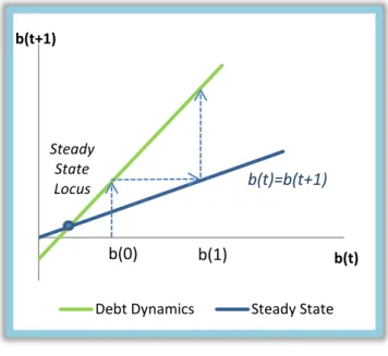
Figure 4 represents the case of Stable Debt Dynamics, where the horizontal axis represents the Debt level in the current and the vertical axis represents the level of Debt in the next period. The case of Stable Debt Dynamics indicates that Debt is growing at decreasing rate. This means that if the situation is left unregulated, the accumulation of Government Debt will stop after some time and come to the Steady State Locus. This implies that every next period b(0), b(1), b(2) etc. the Debt Dynamics function (green line) is approaching the steady state function (blue line) (Figure 4). Along the steady state line government debt stays unchanged, and can be written as bt = bt+1 (blue line). In order for Stable Debt Dynamics to happen, the nominal growth rate of GDP should exceed the interest rate, in other words n>i leading to [(1+i)/(1+n)]<1 in Formula (6). If this holds, assuming that Budget Deficit is 0, the change in Government Debt every next period will be smaller than the previous one.

8

Figure 4: Stable Debt Dynamics

Source: Isaac, 2009

2.2.2

Unstable Debt Dynamics

The second case is Unstable Debt Dynamics, where debt is growing at increasing rates. In this case, the Debt Dynamics level moves farther away from the Steady State Locus every next period.

Figure 5: Unstable Debt Dynamics

Source: Isaac, 2009

Unstable Debt Dynamics process happens when the nominal growth rate is below the interest rate level, in other words n<i leading to [(1+i)/(1+n)]>1 in Formula 6. If this situation is left unregulated, at some point of time the interest payment on Government Debt will exceed the country’s GDP. In this case, the country will go bankrupt due to the Budget Crisis presence.

b(t+1)

b(t)

Steady State Debt Dynamics

b(0) b(1) b(2) b(3) Steady State Locus b(t)=b(t+1) b(t+1) b(t)

Debt Dynamics Steady State

b(0) b(1)

b(t)=b(t+1)

Steady State Locus

9

Government Debt nevertheless does not have automatic correlation with the economic variables. Instead, it is the government policy on Debt repayment, which is causing cer-tain consequences in the economy. The two major policies are: Bond Issuing and Mone-tary, Debt Monetizing in particular. Each of these strategies has effects on the country’s GDP growth but through different variables (Dornbusch & Fischer & Startz, 2004).

2.3

Bond Financing

In case Government finances the accumulated Debt by issuing bonds, the revenues to repay the Debt are collected by selling the bonds to the public. Bond issuance is literary described as government borrowing from the public. This process drives up the interest rates, trying to make the bonds a better alternative for the individuals to use their mon-ey. Nevertheless, the monetary base and the inflation level stay unchanged (McCallum, 1984).

Budget Deficit can be also defined (Fischer & Easterly, 1990) as:

Budget Deficit = (Private Savings – Private Investment) + Current Account Deficit

(7)

Bond Financing policy directly effects the first term on the right side of the Formula 7, (Private Savings – Private Investment). As it is mostly agreed, higher long-term interest rate, arising from the Budget Deficit financing, is crowding out private investments (Hoelscher, 1986).

Crowding Out Effect. If Government is constantly running Budget Deficits, they start accumulating themselves into Government Debt. One way to finance the debt is through Fiscal Expansionary Policy, by increasing expenditures, which is accompanied by bond issuance. This process drives up long-term interest rates making it more attractive for private sector to save instead of invest. Lower Investments level as a result reduces the GDP growth (Fischer & Easterly, 1990). Graphically this situation can be represented as an IS-LM identity, with Money Supply kept fixed (vertical LM curve). The upward shift of the IS curve causes full crowding out of the Investments (Dornbusch & Fischer & Startz, 2004).

Nevertheless, some economists are arguing that Crowding In Effect is more likely to oc-cur instead. Crowding In states that the money, collected from the bonds, are reinvested into the economy, creating larger output and resulting in GDP growth (Eisner, 1989). Such two opposite views on the same problem can be explained by the way the gov-ernment is spending the money. We know that developing countries tend to have higher GDP growth, therefore the government will find it more beneficial to reinvest the mon-ey into the growing economy and the Crowding In effect is more likely to happen (The Economist, Dictionary). In the developed countries, GDP growth is normally much lower; therefore, government will more likely spend the money on debt repayments. The latter process actually means that the government is taking the money from its economy, and immediately pays the foreign country.

From the reasoning above, the Debt increase is boosted when the government borrows from the public, but does not reinvest into the economy the accumulated money, violat-ing the Golden Rule (The Economist, Dictionary).

10

Since this paper is taking a sample of EU countries, the Crowding Out argument holds true, as the countries are developed.

The government can also try to increase investments through the Expansionary Fiscal Policy. In this case, the government can not only increase expenditures, but also cut tax-es. The cut in taxes is done to increase private spending and stimulate the growth of the economy. Nevertheless, Barro-Ricardo effect shows that the desired result is not achieved.

Barro-Ricardo effect states the hypothesis that tax and deficit have an equivalent effect on consumption, and leave investments, trade balance and total demand unchanged. Government increases disposable income of individuals by tax cutting in order to stimu-late higher household spending and growth of the economy. Nevertheless, a tax cut will be automatically accompanied by increased savings. The far-seeing consumer recogniz-es that the increased government debt will soon be financed by tax increase, equal to the amount of tax cut, performed today. The individual prefers to save today in order to be able to pay the expected higher tax in the future (Fischer & Easterly, 1990). If this holds true, private savings are compensating for the government, leaving aggregate savings unchanged. Therefore, crowding out does not happen.

Barro-Ricardo effect has been a topic of active discussions in the economics literature; however, no one has been able to reject completely the hypothesis.

These processes give us the understanding of the Snowball effect, which happens, when higher interest rates decrease growth, pushing the government to increase Debt to GDP ratio, and driving up interest rates again. This process of the vicious circle deepens the country’s indebtedness (Report of the Swedish Fiscal Policy Council, 2010). We have seen that the Bond Issuance policy if used solely can drive up interest rates and decrease GDP growth, pushing the term (1+i)/(1+g) in Formula 6 closer or even higher than 1. We can conclude from these reasoning that the Bond Issuance policy can lead to the Unstable Debt Dynamics.

2.4 Monetary Policy

In this section, I will talk about how the government is financing its debt with the use of Monetary Policy. In particular, the government is Monetizing the Debt, increasing the volume of high-powered money, but targeting to leave the interest rate unchanged. This process implies that Central Bank prints additional money to be able to buy gov-ernment bonds. After this, the govgov-ernment is able to repay the Debt with newly printed high-powered money. The process is targeting to leave the interest rate unchanged, in order to avoid crowding out effect. By rapid increase of money supply, the government is trying to achieve seignorage, higher than the cost of inflation as long as possible (Fischer & Easterly, 1990). Therefore, as long as the inflation is at comparatively mild level, it can do no harm to the economy. European Central Bank sets the inflation target at the level of 2%.

In case of high inflation, there is a negative effect on the GDP growth, especially if high inflation is maintained over a long period. In addition, any government that attempts to inflate away the real value of the short-term Debt will soon find itself paying a much higher nominal interest rate in the long-run (Reinhart & Rogoff, 2010). Other costs are

11

an arbitrary redistribution of wealth and higher inflation risk premium in the interest rates demanded by the investors, if the inflation is high and unexpected (www.ecb.europa.eu).

An important role in the effect of inflation on the economy plays the exchange rate re-gime. In case of floating exchange rate and high inflation, the domestic currency will depreciate, affecting the Current Account and consequently the Balance of Payments, as the country becomes cheaper to the rest of the world. The situation will improve after some time with the increased consumption and investments from the foreigners (Fischer & Easterly, 1990). In case of the fixed exchange rate, the government will try to main-tain the rate as long as it has reserves of foreign exchange and will be able to intervene. However, if the government is run out of foreign exchange, it will eventually devaluate the currency, leading to the process, as with the floating exchange rate (Fischer & Eas-terly, 1990).

The main point is the importance of the effect of the government Debt Financing Policy on the Unstable Debt Dynamics process. As Bond Financing interest rate increases, de-creasing the growth rate, there will be higher probability of interest rate exceeding the GDP growth rate in the long-run, resulting in Unstable Debt Dynamics. Moreover, as the Debt level continues to increase, it is becoming harder for the government to reas-sure the public in the sustainability of its debt, as the country’s default spread enlarges (Damodaran, 2002). On the other hand, Debt Monetizing policy will keep interest rates unchanged, but drive up inflation. As the model is dealing with nominal interest rates and growth, the two terms will be increasing proportionally, adjusting to the inflation. Nevertheless, as rapid inflation continues, people prefer other currencies, which appear to be more stable and government ends up printing even more money (Fischer & Easter-ly, 1990). Persistent high inflation over significant periods causes the decrease in the GDP growth rate (Barro, 1995). This fact can lead to the growth rate falling below in-terest rate, resulting in the Unstable Debt Dynamics as well.

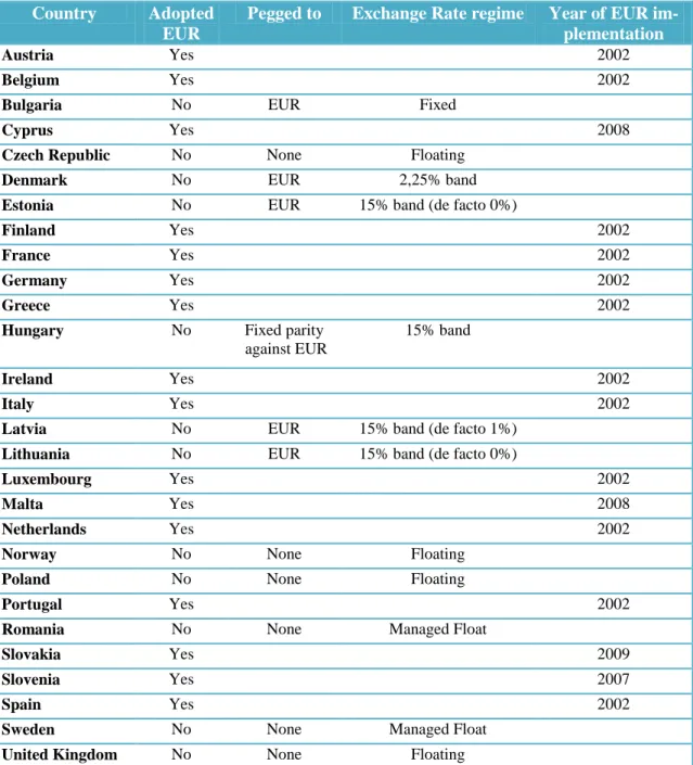
Dealing with EU area, we should take into consideration different currency regimes across the EU (Table 4). Some countries, being a member of the EU, preferred to keep their domestic currencies. These currencies are pegged to EUR, pegged with different bands or are fluctuating. Countries, using their domestic currency with a floating ex-change rate, have the freedom of Monetizing their Debt. Others have a band, within which their currency can fluctuate, which will partly restrict the use of Debt Monetizing policy. On the other hand, countries EMU members adopted EUR, implying their ina-bility to use Monetary policy independently. The next section will give a brief history of the EMU and the role and rules of ECB.

2.5

EMU and ECB

EMU economic integration implies:

Free trade area (with no internal tariffs on some or all goods between the partici-pating countries);

12

Customs Union (with the same external customs tariffs for third countries and a common trade policy);

Single market (with common product regulations and free movement of goods, capital, labor and services);

Common Monetary policy.

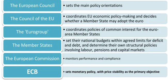
Monetary policy of the euro-using countries is determined by the European Central Bank (ECB). As seen from Figure 6 in the Appendix, ECB is only an institution, which carries out determined policies. ECB has the exclusive right to decide on the volume of the EUR issues (Maastricht Treaty, 1992). This implies that the countries members of EMU cannot use their Monetary Policies and consequently Monetize their Debts. This policy is working fine in peace times, as the countries had to adjust their deficit (below 3% of GDP) and debt (below 60% of GDP) levels in order to qualify for the European Monetary Union acceptance (Stability and Growth Pact). The troubles begin when some countries start violating the rules by accumulating excessive debt levels and have an ur-gent need for the stabilization policies. Then the only option is the Bond Financing strategy, as Maastricht Treaty explicitly forbids ECB to come to the potential defaulter’s rescue (Martino, 2008).

An important point is that in monetary unions, such as EMU, an extraordinary large debt in one country can create pressure on the financial markets of the entire union (Köhler-Töglhofer & Zagle, 2004). This can be a potential threat to the worsening of the Debt Dynamics over the whole group of countries EMU members.

This paper’s focus is kept on the two major groups of countries within the EU: members of EMU and non-members of EMU. The different exchange rate regimes among the non-EMU members are not considered under the analysis, as these countries still have a possibility of devaluation/depreciation.

As we have seen, both policies can cause Unstable Debt Dynamics process, the question is “Can the lack of the possibility of using both Debt financing strategies in EMU coun-tries lead to higher Debt Dynamics level, as compared to the rest of the EU councoun-tries?” This question is hard to test, taking into consideration all aspects of the problem. How-ever, in the next section I will introduce the process, which will try to compare the two groups.

13

3

Statistical Methods and Results

3.1 Data Analysis and Hypothesis

The two datasets have been selected for the analysis: General Government Defi-cit/Surplus and General Government Debt, both measured as percent of GDP (Eurostat Statistics).

In this study I am using the fixed effects for each country’s set of values. This method allows to run a regression, treating the whole data set as individual cases, instead of re-gressing the data without specifying which country it refers to. Therefore, the Fixed Ef-fects method ignores the between-country variation and focuses only on the within-country variation.

The sample period for the analysis has been chosen from 1996 until 2009. This sample period is defined by the analysis of the last decade and the availability of data. For the study the data was organized in the Dated Panel view, allowing for the cross-sectional time series analysis.

The Null Hypothesis is:

H0: Countries EMU-members do not have a higher Debt Dynamics (or are not

lean-ing towards Unstable Debt Dynamics) compared to the countries non-EMU members. In other words, there is no difference in Debt Dynamics level of the two countries’ sets.

OR: β0=β1=β2=β3=0

HA: The difference between the two groups of countries exists, implying that the

EMU-member countries have higher value for Debt Dynamics than the non-members. OR: β3 ≠ 0

3.2 Panel Least Squares Analysis

The regressed formula looks as follows:

t t t t t

BB

GD

EMU

GD

EMU

GD

*

Where GDt+1 is the government Debt of the current period, BBt is the Budget Balance of

the previous period, GDt is the government Debt of the previous period, EMU is the

Dummy variable and t is the error term.

Let us recall Formula 6, where Budget Balance was defined as d = Dpt / YNt and was

sumed to be zero over time. In order to make the study more realistic, we release the as-sumption of no deficit. Therefore, Budget Balance is represented by BB value in the re-gression, lagged one period back.

Government Debt is represented by GD, and is also lagged one period back. For a better representation we will take the derivative of GD(t+1) with respect to GDt, getting the

14 EMU GD GD t t 3 2 1

₍₈₎

As seen from Formula 8, if β2 represents the Debt Dynamics level for non-EMU

coun-tries, (β2 + β3) represents the Debt Dynamics for the EMU countries. Following this

log-ic, β3 represents the difference between the two groups of countries. If H0 for β3 is

re-jected and β3 is positive, this will indicate, that countries-members of EMU have higher

Debt Dynamics; if β3 is equal to 0, EMU countries are not different from the rest of the

countries in their Debt Dynamics trends.

As the research question implies differentiating the countries according to their euro ac-ceptance, we need to consider the fact that the year of its acceptance is individual for every country. Therefore, the Dummy variable, called EMU was created. EMU Dummy returns 0 for all non-EMU countries and for all EMU members before 2002. Therefore, according to Table 4 the EU countries like Austria, Belgium, Netherlands, Finland, France, Germany, Ireland, Italy, Luxembourg, Portugal, Spain and Greece have the EMU-value 0 before 2002. Slovenia has EMU-value 0 before 2007, and Cyprus, Malta and Slovenia before 2009. EMU returns 1 in the rest of the cases, which is the values for the EMU-members after the date of euro introduction.

The coefficients, which are of the greatest interest to us are β2 and β3 as they represent

the ratio (1+i)/(1+n) in Formula 6. Therefore, if β2 or (β2+ β3) coefficients are greater

than 1, the group of countries can be concluded to have Unstable Debt Dynamics. If the coefficients are less than 1 and greater than 0, the Stable Debt Dynamics process is present.

3.3 Regression Results

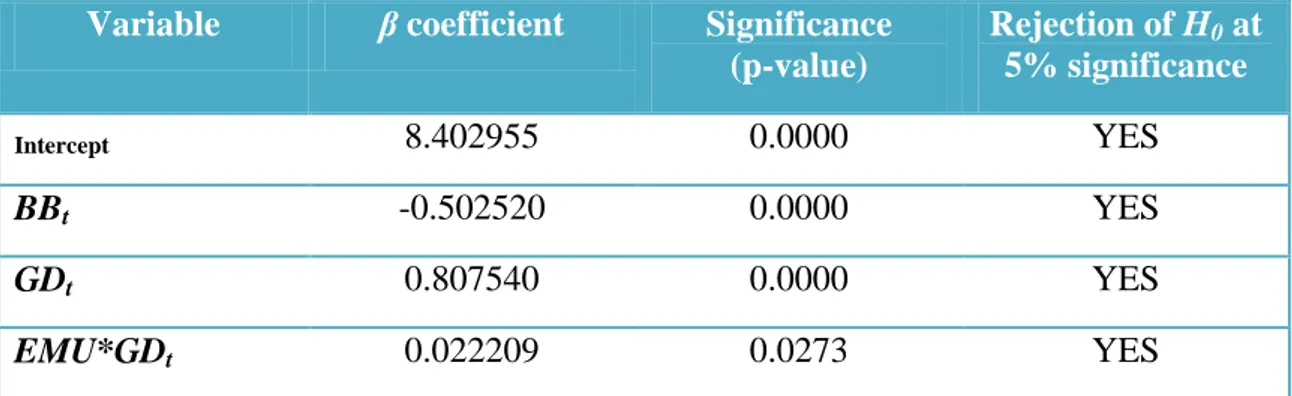
The regression results are shown in Table 3 and the full Output Table can be seen in the Appendix. The hypothesis is tested at 5 % significance level, therefore if the p-value is lower than 0.05, the Null Hypothesis is rejected.

Table 2:

Regression results of Panel Least Squares: Variables, Coefficients

and Significance Levels

Variable β coefficient Significance (p-value) Rejection of H0 at 5% significance Intercept 8.402955 0.0000 YES BBt -0.502520 0.0000 YES GDt 0.807540 0.0000 YES EMU*GDt 0.022209 0.0273 YES

As the p-value for Budget Balance is lower than 0.05, we reject the Null Hypothesis and believe that β1 is equal to -0.502520. This result shows that the Budget Deficit previous

period is negatively correlated with the Government Debt of the current period. This outcome is consistent with the theoretical implication.

15

The p-value of Government Debt previous period is also lower than 0.05, which means that we conclude that β2 is equal to 0.807540. This value indicates that the Debt

Dynam-ics of non-EMU members is Stable. Nevertheless, it is significantly close to exceeding the level of 1, after which the Debt Dynamics become Unstable.

Finally, the p-value for the difference value between the two groups of countries (EMU*GDt) is 0.0273, which is still lower than 0.05. This means that we reject the Null

Hypothesis and believe that β3 is equal to 0.022209. In other words, this finding means

that the countries-members of EMU have higher Debt Dynamics by 0.022209, than the EMU members. We can compare the two groups of EMU members and non-members by looking at two coefficient values of 0.807540 vs. 0.829749 respectively. R2 of the regressionis equal to 0.978 representing a very good fit of the regression and insignificant variation in the error terms.

16

4 Analysis

The results of the regression indicate that the difference between the two groups of countries exists. This difference means that the countries EMU members tend to have higher Debt Dynamics than the non-EMU members. Based on this finding we can sug-gest that extensive usage of Bond Issuance policy does lead to higher Debt Dynamics. This can be due to the fact that Crowding Out process affects two variables: interest rates and GDP growth, involved in the Debt Dynamics process. These variables are in-fluenced in the most positive way for the Snowball effect to start. On the other side are the non-EMU members, who have the choice of Financing Policy. For these countries Monetary policy allows to attract foreign capital when the exchange rates are depreciat-ing. As the historical overview has shown, the problems started due to the countries’ vi-olation of the SGP rules. A reasonable suggestion arises, that once the countries will be able to stabilize their Budget Balances and Debt levels to the SGP levels, the difference between the two groups will disappear.

On the other hand, the difference between EMU and non-EMU members may seem to be quite small. The most critical question that is raised by the results of the performed regression is: Is the difference of 0.022 large enough to conclude about the extensive negative effects of common currency on the Debt Dynamics Development? There are two main arguments that can be proposed for the significance of the obtained value. The first one is that the number of 0.022 may seem small if taken on its own. Neverthe-less, as we know some of the EMU member countries have accumulated extremely large Debt levels. As for example in the cases of Germany, France, UK and Italy, where Debt has passed a trillion EUR level. Consequently, looking at this difference in the money value does generate some significance to the obtained result.

The second argument is attributed to the amount of time, which has passed, since the creation of the Common Currency area. As shown in Table 4, the majority of the coun-tries have implemented EUR in 2002 and some councoun-tries only in the last three years. If looked at the country scale picture, eight years may not be enough for the difference in the Debt Dynamics levels between the two groups of countries to become obvious. Moreover, the recent financial crisis in 2007 has pushed many countries to accumulate additional Debt. This implies that the stabilization and the pay-back period after the cri-sis will create more favorable conditions for the comparison of the countries, using dif-ferent Debt financing policies. These facts propose that the obtained difference of 0.022 can be quite significant for the comparatively short time of EMU existence. Moreover, it may considerably increase with the progress of time.

The two reasoning are emphasizing the importance of careful consideration of the EMU joining. We should keep in mind that this analysis is looking only at one side of the EMU disadvantages, not considering its benefits. The cost-benefit analysis of common currency acceptance should be performed individually, taking into consideration the specifics of each country.

Another finding, which can be observed from the regression’s results, is the high Debt Dynamics level overall. From Table 2 we have seen that the Debt Dynamics value is around 0,8 in both groups. This is definitely close to turning into the Unstable Debt Dy-namics process, which will require much more interference into the economy. This

in-17

teresting result indicates that there is a serious problem of growing Debt in the entire European Union. It is important, that high Debt Dynamics process is present even in the countries, with comparatively low Debt as percent of GDP levels. This finding indirect-ly supports the theory of Debt Intolerance by Reinhart, Rogoff and Savastano, suggest-ing that even low levels of Debt can cause serious risks, like country’s default.

18

5 Conclusions

This thesis is looking at the Debt Financing policies: Bond Issuing and Monetary, Debt Monetizing in particular. The focus is kept on the way these two strategies can contri-bute to the Unstable Debt Dynamics process development through the Snowball effect arising. As the Snowball effect happens through decreased GDP growth, increased in-terest rate or increased inflation, different theories are discussed, linking the Debt fi-nancing policies and the Debt Dynamics.

While discussing the two Debt financing strategies, it gets clear that Bond Financing and Monetizing, if used solely can lead to Unstable Debt Dynamics. Consideration of the EU countries brings up the questions: “What happens to the countries EMU mem-bers? Do they have higher Debt Dynamics level than the rest of the EU memmem-bers?” These questions are reasonable, as the EMU members do not have a choice of Debt Fi-nancing policy and have to follow the ECB Monetary policy rules. Theoretical frame-work on Debt Dynamics discusses in detail, how likely it is that the EMU countries will have the Unstable Debt Dynamics.

My empirical findings indicate that EMU member countries have higher Debt Dynam-ics by 0.022, compared to the non-EMU members. This result has been obtained after performing the Paned Least Square Analysis (with fixed effects), supporting the theoret-ical framework. This result can be explained explained by the fact that as the EMU members excessively use Bond Financing strategy, Crowding Out effect becomes larg-er, starting the Snowball effect and increasing the Debt Dynamics. The difference of 0.022 also appears to be not so small if looking at the money value of accumulated Debt. In addition, this difference has been accumulated only after eight years of EMU existence, which suggests that it can be increasing with time.

Another interesting result of the performed regressions indicates that both groups of countries, EMU and non-EMU members, have quite high level of Debt Dynamics (around 0.8). This value is considered high, as the Unstable Debt Dynamics start, as soon as this value exceeds 1.

The two observed results indicate the importance of the proper Debt Financing strategy choice and the significance of Monetary Policy. Moreover, the discovered difference in the two groups of countries indicates that there is a room for further research in this field.

5.1 Suggestion for Further Research

This paper discusses in detail variables, involved in the Debt Dynamics process. Never-theless, these variables (GDP growth, interest rate and inflation) were not quantitatively included into the analysis. I would suggest to develop the model, which would include these variables and investigate which one had the greatest influence on the Debt Dy-namics process.

Another suggestion would be to perform the same analysis after the stabilization period of the recent financial crisis. This way it would be easier to see, how the countries were able to finance their rapidly increased debt and which group performed better in terms of Debt Dynamics levels.

19

6 References

6.1 Scientific Publications

1. Roubini N., Sachs J. (1988). Political and Economic Determinants of Budget Defi-cits in the Industrial Democracies. National Bureau of Economic Research, Cam-bridge.

2. Reinhart C., Rogoff K., Savastano M. (2003). Debt Intolerance. Brookings Papers on Economic Activity, Vol. 2003, No. 1 (2003), p. 1-62

3. Rogoff K. (2010). Growth in a Time of Debt. American Economic Review Papers and Proceedings. Harvard University and NBER.

4. Barro R. (1995). Inflation and Economic Growth. National Bureau of Economic Research, Cambridge.

5. Damodaran A. (2002). Investment Valuation. Tools and Techniques for Determin-ing the Value of Any Asset (2nd ed.). John Wiley & Sons, Inc., New York.

6. Shojai S. (1999). Budget Deficits and Debt: a Global Perspective. Greenwood Pub-lishing Group, Incorporated. Westport, Connecticut London.

7. Köhler-Töglhofer W., Zagler M. (2004). The impact of Different Fiscal Policy Re-gimes on Public Debt Dynamic.

8. McCallum B. T. (1984). Are Bond-financed Deficits Inflationary? A Ricardian Analysis. The Journal of Political Economy, Vol. 92, p. 123-135

9. Fischer S., Easterly W. (1990). The Economics of Government Budget Constraint. The World Bank Research Observer, Vol. 5, No. 2, p. 300-308

10. Isaac A.G. 2009. Course: Macroeconomics. Debt and Deficit.

11. Dornbusch R., Fischer S., Startz R. (2004). Macroeconomics. International Edition. McGraw-Hill, New York.

12. Hoelscher G. (1986). New Evidence on Deficits and Interest Rates. Journal of Money, Credit and Banking, Vol. 18, No. 1, p. 1-17.

13. Eisner R. (1989). Budget Deficits: Rhetoric and Reality. The Journal of Economic Perspectives, Vol. 3, No. 2, p. 73-93.

14. Vieira C. (2000). Are Fiscal Deficits Inflationary? Evidence for the EU. Depart-ment of Economics, Loughborough University, UK.

15. Argimon I., Gonzalez-Paramo J., Roldan J. (1997). Evidence of Public Spending Crowding Out from a Panel of OECD countries. Applied Economics, 1997, 29, p. 1001-1010.

16. Martino A. (2008). Milton Friedman and the Euro. Cato Journal, Vol. 28, No. 2, 2008.

20

17. Maastricht Treaty (1992). Provisions Amending the Treaty Establishing the Euro-pean Economic Community with a View to Establish the EuroEuro-pean Community. Maastricht.

18. Swedish Fiscal Policy (2010). Report of the Fiscal Policy Council 2010. Principal conclusions and Summary.

6.2 Websites

1. European Commission, Eurostat (1953). General government deficit (-) and surplus (+); Percent of GDP. Data retrieved on March 19, 2010, from

http://epp.eurostat.ec.europa.eu/tgm/table.do?tab=table&init=1&plugin=1&languag e=en&pcode=teina200

2. European Commission, Eurostat (1953). General government debt; percent of GDP. Data retrieved on May 16, 2010, from

http://epp.eurostat.ec.europa.eu/tgm/table.do?tab=table&plugin=1&language=en&p code=tsieb090

3. European Commission, Eurostat (1953). Short-term and long-term interest rates. Data retrieved on June 10, 2010, from

http://appsso.eurostat.ec.europa.eu/nui/setupModifyTableLayout.do

http://appsso.eurostat.ec.europa.eu/nui/show.do?dataset=irt_lt_gby10_a&lang= en

4. European Commission, Eurostat (1953). Annual change of GDP in percent. Data retrieved on June 10, 2010, from

http://appsso.eurostat.ec.europa.eu/nui/show.do

5. Organization for economic co-operation and development, OECD Statistics (1961). Central government debt; percent of GDP. Data retrieved on March 17, 2010, from

http://stats.oecd.org/index.aspx

6. Organization for economic co-operation and development, OECD Statistics (1961). Total expenditure of general government; percent of GDP. Data retrieved on March 20, 2010, from http://stats.oecd.org/index.aspx

7. Budget Balance. Economist.com. Retrieved May 15, 2010, from

http://www.economist.com/research/economics/searchActionTerms.cfm?query= budget+balance

8. Debt. Economist.com. Retrieved May 15, 2010, from

http://www.economist.com/research/economics/searchActionTerms.cfm?query= debt

9. Golden Rule. Economist.com. Retrieved May 15, 2010, from

http://www.economist.com/research/economics/searchActionTerms.cfm?query= golden+rule

21 10. European Monetary Union information

http://ec.europa.eu/economy_finance/euro/index_en.htm

11. European Central Bank information

22

Appendix

Table 3:

EU countries’ currency use and exchange rate regimes

EUR

Pegged to Exchange Rate regime Year of EUR im-plementation

Austria Yes 2002

Belgium Yes 2002

Bulgaria No EUR Fixed

Cyprus Yes 2008

Czech Republic No None Floating

Denmark No EUR 2,25% band

Estonia No EUR 15% band (de facto 0%)

Finland Yes 2002

France Yes 2002

Germany Yes 2002

Greece Yes 2002

Hungary No Fixed parity against EUR

15% band

Ireland Yes 2002

Italy Yes 2002

Latvia No EUR 15% band (de facto 1%)

Lithuania No EUR 15% band (de facto 0%)

Luxembourg Yes 2002

Malta Yes 2008

Netherlands Yes 2002

Norway No None Floating

Poland No None Floating

Portugal Yes 2002

Romania No None Managed Float

Slovakia Yes 2009

Slovenia Yes 2007

Spain Yes 2002

Sweden No None Managed Float

United Kingdom No None Floating

Sources: Eurostat Publications, Riksbank, Norges Bank, Bank of England, http://www.euro-dollar-currency.com/history_of_euro.htm

23

Figure 6: European Monetary Union Institutional Structure and the Role of

European Central Bank

Output Table: Panel Least Squares Analysis

Dependent Variable: GD Method: Panel Least Squares Date: 05/14/10 Time: 17:31 Sample (adjusted): 1997 2009 Cross-sections included: 28

Total panel (unbalanced) observations: 354

Variable Coefficient Std. Error t-Statistic Prob.

C 8.402955 1.415705 5.935526 0.0000

BB(-1) -0.502520 0.106015 -4.740097 0.0000

GD(-1) 0.807540 0.028149 28.68819 0.0000

EMU*GD(-1) 0.022209 0.010016 2.217332 0.0273

Effects Specification Cross-section fixed (dummy variables)

R-squared 0.978291 Mean dependent var 48.85395

Adjusted R-squared 0.976275 S.D. dependent var 26.89086

S.E. of regression 4.141967 Akaike info criterion 5.763715

Sum squared resid 5541.352 Schwarz criterion 6.102552

Log likelihood -989.1776 F-statistic 485.1967

Durbin-Watson stat 1.159760 Prob(F-statistic) 0.000000

• sets the main policy orientations

The European Council

• coordinates EU economic policy-making and decides whether a Member State may adopt the euro

The Council of the EU

• coordinates policies of common interest for the euro-area Member States

The 'Eurogroup'

• set their national budgets within agreed limits for deficit and debt, and determine their own structural policies involving labour, pensions and capital markets

The Member States

• monitors performance and compliance

The European Commission

• sets monetary policy, with price stability as the primary objective

ECB