Quality assurance for magnetic resonance imaging (MRI) in radiotherapy

(1)

Quality Assurance for Magnetic

Resonance Imaging (MRI) in

Radiotherapy

Mary Adjeiwaah

Thesis for the degree of Licentiate

Thesis Advisors: Tufve Nyholm PhD, Joakim Jonsson PhD, Anders

Garpebring, PhD

(2)

This Project has been funded by the Schlumberger Faculty for the Future Foundation (FFTF) © Mary Adjeiwaah 2017

Medical Faculty , Department of Radiation Sciences ISBN: 978-91-7601-797-5 (print)

ISBN: 978-91-7601-797-5 (pdf )

This work is protected in accordance with the Swedish Copyright law ( Act 1960:729) Responsible publisher under Swedish Law: Dean of the Medical Faculty

(3)

(4)

(5)

List of Figures

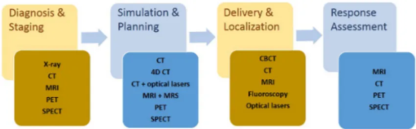
1.1 Medical imaging modalities at each phase of the radiotherapy process. Modiﬁed from

http://www.radiationoncology.com.au/resourcing-the-radiation-oncology-sector/essential-imaging-and-radiotherapy-techniques/

4

2.1 Proton precession due to an applied magnetic ﬁeld. The

intrin-sic properties of a Hydrogen proton utilized by MRI: spin [de-scribing inherent angular momentum] and magnetic moment, (a). Precession of charged particles in the direction of the applied external magnetic ﬁeld, (b). . . 11 2.2 Magnetic resonance (MR) signal decay. Before the 90o

radio-frequency (RF) pulse, the net magnetization (Mo) from all spins

point in the direction of the main magnetic ﬁeld (z-axis) [a]. By applying a 90o_{RF pulse, the spins gain energy and M}

0is ﬂipped

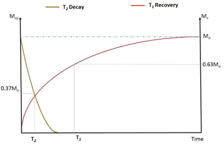
into the transverse plane to produce measurable MR signal [b] but because of local magnetic ﬁeld inhomogeneities, spins get out of phase and the net magnetization returns to equilibrium. This rapid decay of signals induced in the receive coils is known as Free Induction decay. . . 13 2.3 Magnetization time curve. Longitudinal magnetization recovery

governed by T1relaxation time occurring at the same time as the

decay of the transverse magnetization governed by T2relaxation

(8)

2.4 Pulse Sequence diagram for magnetic resonance image forma-tion simpliﬁed for Gradient Echo. A radio-frequency (RF) pulse

combined with the slice select gradient (Gss) selectively excite

the region of interest. The Phase (GP E) and frequency (GF E)

encoding gradients are for spatial encoding of the signals. To re-phase all de-re-phased transverse magnetizations, additional gradi-ents (outlined in red) are applied after slice selection and before frequency encoding. Modiﬁed from the book, ’ MRI from Picture

to Proton’, 3rdedition [1] . . . . 15 2.5 Filling of K-space after magnetization. After RF excitation and

before any gradients, all encodings will be at (a). The application of a negative phase encoding gradient moves all data to point (b) where upon applying a frequency encoding gradient, the data is sampled along Kf e, from b to d. Modiﬁed from the book, ’ MRI from Picture to Proton’, 3rd edition . . . . 17 3.1 Linear and Nonlinear gradients. Variations in location of signals

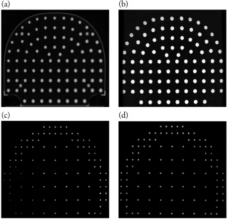
due to nonlinear ﬁeld gradients. . . 20 3.2 Axial Images of the GE and Spectronics phantoms used in this

study. Computed Tomography and Gradient echo Magnetic

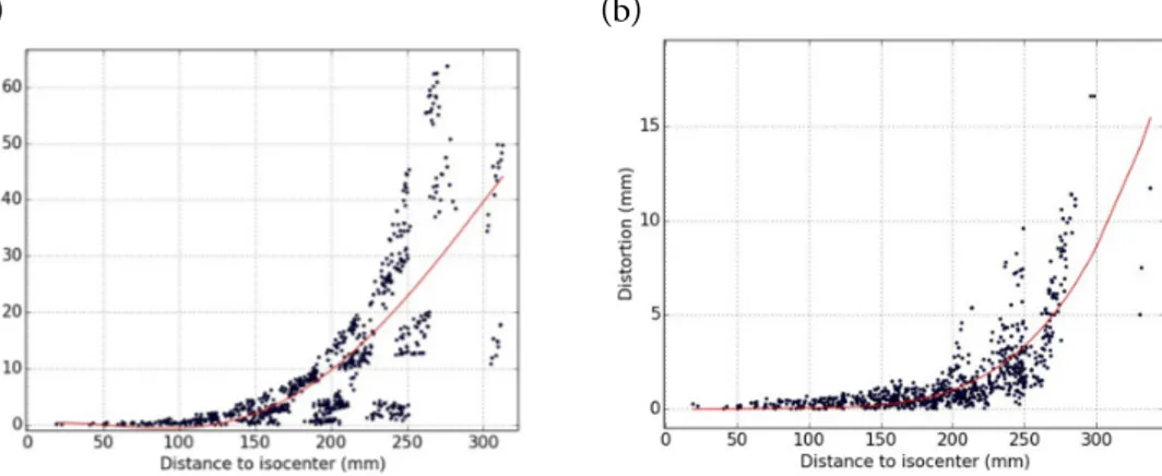
res-onance images of the Spectronics (a & b) and GE (c & d) large ﬁeld of view spatial analysis phantoms. . . 24 3.3 Reduction in Gradient Nonlinearity distortions with 3D

cor-rection. Magnitude of MR Nonlinearity distortions with radial

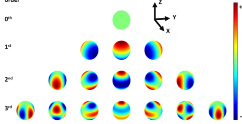
distance from the isocenter without 3D correction (a) and with 3D correction for a spin echo sequence using a bandwidth of 488 Hz/pixel. . . 26 3.4 Spherical harmonics (SH) up to third-order. High SH orders

result in increasing number of modeled shapes. This in turn in-creases the likelihood to improve the B0 homogeneity. SH are

arranged in orders of N with 2N + 1 terms for each order. . . 27 3.5 Reduction in magnitude of residual system distortions with

in-creasing bandwidth. Phantom measured residual system

distor-tions decreased in magnitude with increasing bandwidth from 122 Hz/pixel (a) to 244 Hz/pixel after 3D correction . . . 29

(9)

3.6 Shifts due to system- and patient-induced susceptibility distor-tions. Estimated shifts at the contours of the bladder, the femoral

heads, planning target volume (PTV) and rectum at bandwidths of (a) 122 Hz/pixel, (b) 244 Hz/pixel, (c) 488 Hz/pixel in the right to left gradient readout. The boxes show the average values of the median (centerline) and 25% and 75% percentiles (bot-tom and top of boxes for all patients, in millimeters. The points above and below each box represent the range in absolute shifts. L = left; R = right . . . 32 3.7 Contour overlap between distorted and original CT datasets.

Dice similarity coeﬃcient (DSC) at some selected contours and the two bandwidths studied. The mean agreement between dis-torted CT and original patient CT for all patients were above 0.9 except for the spinal cord at the 122 Hz/pixel. [B-Brain,

C-clinical target volume, L-left parotid, R-Right parotid, P-Planning target volume, S-spinal cord] . . . . 33

(10)

(11)

List of publications

This thesis is based on the following publication and Manuscript:

1 Quantifying the Eﬀect of 3 T Magnetic Resonance Imaging Residual System Distortions and Patient-Induced Susceptibility Distortions on Radiation Therapy Treatment Planning for Prostate Cancer

Adjeiwaah M, Bylund M, Lundman J.A, Thellenberg Karlsson C, Jonsson JH, Nyholm T

International Journal of Radiation Oncology • Biology • Physics (2017),

doi: 10.1016/j.ijrobp.2017.10.021.

2 Dosimetric Impact of MR distortions - A study on Head and Neck Cancer Patients

Adjeiwaah M, Bylund M, Lundman J.A, Zackrisson B, Söderström K, Jonsson JH, Garpebring A, Nyholm T

(12)

(13)

Abbreviations

Acronyms

3D-CRT three dimensional conformal radiation therapy BW bandwidth

CT Computed Tomography dCT distorted CT

18F-FDG 18F-ﬂuorodeoxyglucose FID Free Induction Decay

FoV Field of View GE Gradient Echo HU Hounsﬁeld unit

IMRT Intensity-Modulated Radiation Therapy MR Magnetic Resonance

MRI Magnetic Resonance Imaging OAR organs at risk

PET Positron Emission Tomography PTV planning target volume

(14)

RF Radio-Frequency RT Radiotherapy

sCT synthetic Computed Tomography (CT) SE Spin Echo

SNR signal-to-noise ratio

SPECT Single-Photon Emission Computed Tomography TE Echo time

TR Repetition time US Ultrasound

(15)

Popular summary

Magnetic resonance imaging (MRI) utilizes the magnetic properties of tissues to generate image-forming signals. MRI has exquisite soft-tissue contrast and since tumors are mainly soft-tissues, it offers improved delineation of the target volume and nearby organs at risk. The proposed Magnetic Resonance-only Radiotherapy (MR-only RT) work flow allows for the use of MRI as the sole imaging modal-ity in the radiotherapy (RT) treatment planning of cancer. There are, however, issues with geometric distortions inherent with MR image acquisition processes. These distortions result from imperfections in the main magnetic field, nonlinear gradients, as well as field disturbances introduced by the imaged object. In this thesis we quantified the effect of system related and patient-induced susceptibility geometric distortions on dose distributions for prostate as well as head and neck cancers. Methods to mitigate these distortions were also studied.

In Study I, mean worst system related residual distortions of 3.19, 2.52 and

2.08 mm at bandwidths (BW) of 122, 244 and 488 Hz/pixel up to a radial dis-tance of 25 cm from a 3 T PET/MR scanner was measured with a large ﬁeld of view (FoV) phantom. Subsequently, we estimated maximum shifts of 5.8, 2.9 and 1.5 mm due to patient-induced susceptibility distortions. VMAT-optimized treatment plans initially performed on distorted Computed Tomography (dCT) images and recalculated on real Computed Tomography (CT) datasets resulted in a dose diﬀerence of less than 0.5%.

The magnetic susceptibility diﬀerences at tissue, metallic, air and bone in-terfaces result in local B0 magnetic ﬁeld inhomogeneities. The distortion shifts

caused by these ﬁeld inhomogeneities can be reduced by shimming. Study II aimed to investigate the use of shimming to improve the homogeneity of local

B0 magnetic ﬁeld which will be beneﬁcial for head and neck cancer

radiother-apy applications. A shimming simulation based on spherical harmonics modeling was developed. The spinal cord, an organ at risk and surrounded by bone and

(16)

in close proximity to the lungs may have high susceptibility diﬀerences. In this region, mean pixel shifts caused by local B0ﬁeld inhomogeneities were reduced

from 3.47± 1.22 mm to 1.35 ± 0.44 mm and 0.99 ± 0.30 mm using ﬁrst and second order shimming respectively. This was for a bandwidth of 122 Hz/pixel and an in-plane voxel size of 1× 1 mm2_{. Also examined in Study II as in Study}

I, was the dosimetric eﬀect of geometric distortions on 21 Head and Neck cancer

treatment plans. The dose diﬀerence in D50 at the PTV between distorted CT

and real CT plans was less than 1.0%.

In conclusion, the effect of MR geometric distortions on dose plans was small. Generally, we found patient-induced susceptibility distortions were larger com-pared with residual system distortions at all delineated structures except the exter-nal contour. This information will be relevant when setting margins for treatment volumes and organs at risk. The current practice of characterizing MR geomet-ric distortions utilizing spatial accuracy phantoms alone may not be enough for an MR-only radiotherapy work flow. Therefore, measures to mitigate patient-induced susceptibility effects in clinical practice, especially patient-specific correc-tion algorithms are needed to complement existing distorcorrec-tion reduccorrec-tion methods such as high acquisition bandwidth and shimming.

(17)

Populärvetenskaplig

sammanfattning

Magnetresonansbildtagning (MR) använder vävnaders magnetiska egenskaper för att generera bildgivande signaler. MR har utmärkt mjukvävnadskontrast, och ef-tersom tumörer främst drabbar mjukvävnad bidrar MR till förbättrad utritning av behandlingsvolymer och närliggande riskorgan. Ett arbetsflöde som endast an-vänder sig av MR-bilder vid planering av strålterapi för cancerpatienter har före-slagits. Det finns dock problem med geometriska distorsioner som beror på hur MR-bilderna samlas in. Dessa distorsioner kommer från ojämnheter i magnetfäl-tet, ickelinjära gradienter och förvrängningar av magnetfältet som orsakas av det objekt som man tar bilder av. I den här avhandlingen har vi kvantifierat effekterna av de geometriska distorsionerna från systemberoende effekter och patientindu-cerade susceptibilitetseffekter både för patienter med prostatacancer och patienter med cancer i huvud/hals-regionen. Metoder för att minska effekterna från dessa distorsioner har också studerats.

I Artikel I mätte vi systemberoende distorsioner från en 3 T PET/MR ka-mera med ett fantom för stort Field of View (FoV). Medel för de största distor-sionerna uppmättes till 3,19, 2,52 och 2,08 mm vid bandbredder (BW) på 122, 244 och 488 Hz/pixel upp till ett radiellt avstånd från isocenter på 25 cm. De största förskjutningarna från patientinducerade distorsioner uppskattades till 5,8, 2,9 respektive 1,5 mm. VMAT-optimerade behandlingsplaner beräknades först på distorderade CT-bilder (dCT) och räknades sedan om på ursprungligt CT-data. Den resulterande dosskillnaden mellan de två dataseten blev mindre än 0,5%. De magnetiska susceptibilitetsskillnaderna i gränsskikt mellan vävnad, metall, luft och ben resulterar i inhomogeniteter i det lokala statiska magnetfältet. Förskjutning-arna som orsakas av dessa inhomogeniteter kan reduceras med shimning. I Artikel II undersökte vi användandet av shimning för att förbättra homogeniteten av det

(18)

lokala statiska magnetfältet. Detta kommer till nytta för användning av MR vid huvud/hals radioterapi. En simulering av shimning baserad på modeller av sfäriskt harmoniska funktioner utvecklades. Ryggmärgen är ett riskorgan som ligger nära lungorna och är omringat av ben, och kan därför ha höga skillnader i susceptibilitet i sin närhet. För denna region kunde medelvärdena för de pixelförskjutningar som orsakats av inhomogeniteter i det lokala statiska fältet minskas från 3, 47± 1, 22 mm till 1, 35± 0, 44 mm och 0, 99 ± 0, 30 mm genom att använda första- re-spektive andra-ordningens shimning vid en bandbredd på 122 Hz/pixel och en voxelstorlek i planet på 1× 1 mm2. I Artikel II undersöktes också den dosimetris-ka eﬀekten av geometrisdosimetris-ka distorsioner på dosplaner för 21 patienter med cancer i huvud/hals-regionen. Dosskillnaden mellan planer beräknade på distorderad CT och ursprunglig CT i D50för PTV var mindre än 1,0%.

Sammanfattningsvis var effekten av geometriska distorsioner i MR-bilderna på dosplanerna små. Generellt fann vi att distorsioner från patientinducerade suscep-tibilitetseffekter var större än distorsionerna från kvarstående systemeffekter för alla utritade strukturer utom patienternas externa konturer. Vi anser att denna information kommer att vara relevant när man sätter säkerhetsmarginaler för be-handlingsvolymer och riskorgan. Man ser även att dagens metoder att utvärdera geometriska distorsioner för MR enbart baserat på fantom för spatiell noggrann-het kanske inte räcker till för ett strålterapiarbetsflöde som enbart baseras på MR-bilder. Av denna anledning krävs utöver existerande distorsionsreducerande me-toder som hög bandbredd och shimning även meme-toder för att minska effekten av patientinducerade susceptibilitetseffekter, till exempel patientspecifika korrige-ringsalgoritmer.

(19)

Acknowledgements

Throughout this work, I have received enormous support from some really impor-tant people in my life. I thank God and my parents for my faith, which consimpor-tantly gives me hope and calms my soul. My dad of blessed memory has been and con-tinues to be my number one cheerleader. Though not physically here, he is my ﬁrst go-to-person when the going gets tough. I don’t know how he does it but he still keeps me calm and motivated. Thank you to my Mom and siblings.

Tufve, you believed in me and gave me an opportunity of a life time. You do not only care for my academic life but are also concerned about the welfare of my family and I thank you for that. In you I have found a good, dedicated and caring supervisor.

Jocke, thank you for being there for me. I come to you unannounced with numerous questions and yet you ﬁnd time to answer them. Thank you for reviews on my write ups.

Anders, you take your time to explain the most complex physics phenomena in the most simplest way you can. Thank you for the many discussions we have had on Matlab and MR physics.

Mikael, what would my academic life be without you, you are a great friend. It means a lot to me especially, when you say, ’Yes. You can do it, I have faith in

You’. I don’t know if I bother anyone more than I do to you, and yet you make

time to ﬁnd all the missing spaces, commas and periods in my write-ups Thank you!. Josef, my go-to-person when the programming gets tough, thank you for the many academic discussions we have had. Thank you for your honest opinions and for your contributions to our review discussions.

Kristina, thank you for our academic and non-academic discussions and for the hugs. Even in tough times we ﬁnd the opportunity to see the brighter side of things. You are a great friend and I could not have asked for a better oﬃce-mate. Jennifer, thank you for your strength, smile, hugs, chit-chats, and dedication

(20)

to the collection of Starbucks city mugs.

Lars, thank you for being a good fellow PhD student and for constantly

re-peating the correct pronunciation of your son’s name when I ask.

Patrik, thank you for your continuous help and patience, especially during my early days here. For fixing my computer and taking just seconds to fix Matlab codes which I had spent days trying to fix.

To Mattias, thank you for answering all my questions about MICE and MIQA and for the many times you had to come to my oﬃce to ﬁx issues with MICE and MIQA

Jón, thank you for the late night MR scans and the light-hearted conversations we have had during ﬁka and late lunch times.

Natalia, for your short time here, you have been a great emotional and aca-demic support, I will miss our chats about our families. Thank you for being there.

Maria, thank you for being Maria, always helpful with all administrative stuﬀ. For your smile and words of encouragement.

My sincere thanks also go to Jonna, Anna, Nadja, Anne, Margareta, Elin, Angelica, Magnus K., Jan, Elisabet, Marita, Tommy, Jörgen, Pia, Helena, Angelica and all the workers at CMTS for sharing this journey with me.

MR. Ali, Zainab, Amal, Jamal, Nana Aisha, Evans, Obaa Aﬁa, Papa Yaw, Ab-dullai, Maxcell, and Jordan, you gave me a family here in Umeå and I am most grateful. To the home front, Thank you Solomon for your Love and for shar-ing this journey with me and our kids. You have given me the opportunity and the room to spread my wings in order to be the woman I want to be. You have made our current living arrangement work with your monthly visits without any complaints. I Love you.

To the composer of the song Daddy ist Doktor, Mama ist zuhause that got me thinking about resuming my academic career, my ﬁrst baby, Awuraa, you are too wise for your age. You are my little girl and yet so matured, caring and helpful. Thank you. To Nana, the little man of the house, you could not be bothered with a lot of things except maybe dinosaurs and music from One direction , Thank you. To Awuraa and Nana, I hope that when you grow up, you will remember your childhood with fond memories. I also hope that the many places we have lived and the travels we have made in our quest to give you a better future will make you grow into better human beings, who will accept and love others as they. And respect the earth that God has made for us. I love you.

(21)

Introduction

The continuous improvement in the diagnosis, staging, before- and after- treat-ment monitoring of cancers within the Radiotherapy (RT) community can be attributed to advances in medical imaging technologies. Medical imaging tech-nologies such as MRI, CT, Ultrasound (US), Positron Emission Tomography (PET), and Single-Photon Emission Computed Tomography (SPECT) are cur-rently available for use in most cancer treatment centers. The last decades have seen the rising use of MRI in RT for treatment planning and image guidance with the introduction of dedicated MR-only simulation scanners for RT plan-ning and hybrid MR-Linac systems [2, 3, 4, 5, 6] for clinical use. In comparison with ionizing radiation-based imaging, MRI provides an exceptional combination of radiation safety and soft-tissue contrast. MRI generate images with stunning clarity of tissue boundaries and can also depict functional properties such as perfu-sion and metabolism. There are, however, issues with geometric distortions inher-ent to MR image acquisition processes hampering the integration of MRI in RT. These distortions result from imperfections in the main magnetic field, nonlinear gradients as well as field disturbances introduced by the imaged object. Current mechanisms to reduce the magnitude of geometric distortions include: (1) the use of manufacturer supplied 3D algorithms to correct gradient non-linearity distor-tions, (2) use of shim coils, which, though limited by rapid variations in the local magnetic field, can mitigate susceptibility effects, and (3) use of high acquisition bandwidths (BW) to reduce both system and patient related distortions, however, increasing BW compromises image quality (signal-to-noise ratio). Lastly, incor-porating acquisition sequences that are less sensitive to field inhomogeneities, such as spin-echo protocols, could be used when necessary to reduce MR spatial inac-curacies. The move towards an MR-only radiotherapy means that existing quality assurance (QA) measures at MR imaging centers will have to be carefully looked at and reviewed to meet the new demands. In this thesis, we investigate the com-bined effect of system related and patient-induced susceptibility distortions on

(22)

radiotherapy treatment planning of prostate as well as head and neck cancers. We also report on mitigations aimed at reducing the eﬀect of distortions on treatment planning.

(23)

Chapter 1

Radiotherapy

1.1 Radiotherapy Treatment planning

Cancer is a major cause of death with 8.2 million global deaths in 2012 and an estimated 14.1 million new cases per year [7]. According to the world cancer report, 20 million new cancer cases have been predicted by the year 2025 [8]. In 2011, of the 57 726 cancer cases reported in the Swedish Cancer registry, 46 286 cases were people who were diagnosed for the ﬁrst time [9]. Prostate cancers are the highest in men representing 32.2% of all cancers in men in 2011. The most common cancer in women is in the breast which accounted for 30.3% of all cancer cases among women in 2011. The continuous ageing of the Swedish population accounts for 50% of the annual 2.1% and 1.5% increase in cancer cases amongst men and women reported over the last two decades. Improvements in the accessibility of diagnostic and screening services also helps explain the increase. Also the risk of developing any form of cancer in Sweden before age 75 is about 31.6% in men and 28.7% in women.

A person diagnosed with cancer will go through one or a combination of treatments involving, surgery, chemotherapy and radiotherapy (RT). At least one in two people with cancer will at some point in their treatment go through RT [10, 11]. In RT treatment, high-energy ionizing radiation from X-ray photons, proton or electron beams are used to kill or restrain the growth of cancer cells.

Normal healthy cells do not divide as rapidly as cancer cells. Therefore when cancer cells are hit and damaged with radiation they cannot repair as eﬀectively as normal cells. RT treatment, makes optimal use of the instability within tumor cells by administering prescribed doses in multiple fractions that normal cells can

(24)

tolerate. For example, the commonly used therapeutic dose of 2 Gy per fraction results in overnight recovery and repair of 99% of double-strand breaks in normal tissues [12].

RT can be delivered in two ways; External or Internal. In external beam ra-diotherapy (EBRT), radiation beams from linear accelerators, cyclotrons or syn-chrotrons outside the body delivers radiation to the target region. Internal ra-diation therapy includes Brachytherapy and the use of radioactive liquids. In Brachytherapy, highly radioactive sources are placed in or near the tumor and then removed after a short time. Alternatively, low radioactive sources known as brachytherapy seeds are left permanently in the patient whilst their radioactivity levels reduce to zero with time.

RT is a localized treatment regime with the primary goal to target malignant tumor cells with maximum dose while reducing dose to normal tissues. This, in turn, improves local tumor control and minimize side eﬀects. Advances in medical imaging technologies have made it possible to deﬁne and treat the tumor with high precision. Dose adjustment during treatment to anatomic regions prone to movement such as the lungs and prostate are also possible. Methods such as three dimensional conformal radiation therapy (3D-CRT), Intensity-Modulated Radiation Therapy (IMRT), and Volumetric-Modulated Arc Therapy (VMAT) combined with image-guided radiation therapy (IGRT) increases the accuracy of dose delivery.

1.1.1 Medical imaging in Radiotherapy

Every stage of current radiotherapy treatment process involves some form of med-ical imaging as speciﬁed in Figure 1.1.

Figure 1.1: Medical imaging modalities at each phase of the radiotherapy pro-cess. Modiﬁed from

(25)

1.1.2 Diagnosis and Staging

In order to optimize treatment, the correct diagnostic information about the loca-tion of the tumor and nearby organs at risk (OAR) will be required. The imaging done at this stage is aimed at determining the location, size, extent, and stage of the tumor including the metastatic status of the disease. The imaging systems in-volved in diagnosing and staging the disease need to have veriﬁable quantitative abilities. These qualities will be most essential when evaluating treatment response and also for future longitudinal studies.

1.1.3 Simulation and Planning

The imaging done here is to simulate the required patient position during the ac-tual treatment. It also involves contouring of the tumor/target volume and accu-rately deﬁning nearby organs-at-risk. For most cancer treatment centers, a CT scan is the gold standard in contouring as well as calculating the needed dose to be delivered during treatment. Tumors are mostly soft-tissues, so MRI with its superior soft-tissue contrast compared to CT might be the preferred choice. Functional imaging approaches such as PET and SPECT can also be used in de-lineating the target volume. There is strong evidence pointing to the advantages of using multi-modal imaging through registration (CT-PET/SPECT, PET-MRI or CT-MRI fusion) techniques to accurately deﬁne the target and OAR.

1.1.4 Dose Delivery and Tumor Localization

With the implementation of image guided radiotherapy, imaging modalities such as cone beam CT (CBCT), MRI, etc. can be used during the delivery of dose to monitor changes in tumor and nearby organs. These changes may be due to bladder and rectal filling as well as lung movements during breathing cycles. In brachyterapy of gynecological cancers and high dose rate prostate brachytherapy, MRI is mostly used to ensure the accurate delivery of dose to the tumor volume. By incorporating imaging during dose delivery, the potential side effects of ra-diotherapy treatment can be greatly reduced [13]. However, CBCT have been associated with impaired visualization of regions with high motion and swallow-ing as well as poor soft-tissue contrast. MRI with its superior soft-tissue contrast may offer a better option for treatment monitoring during dose delivery but, high motion and swallowing may also be a drawback.

(26)

1.1.5 Response Assessment and Follow up

Response assessment involves deciding if a patient is in a remission or there is evidence of the existence of active tumor cells after radiotherapy treatment. Pos-sible tumor metastasis can also be detected during this stage. Each cancer type will respond differently to radiotherapy based on resistance parameters such as hy-poxia, proliferation levels, and intrinsic radiation resistance at the tumor cellular level [14]. The use of medical imaging provides non-invasive monitoring of tu-mor changes during radiotherapy. In head and neck cancers, studies have shown significant reduction in unnecessary salvage surgery due to the accurate depiction of outcome when using 18F-fluorodeoxyglucose (18F-FDG) PET to assess post treatment response [15, 16].

The relevance of imaging in radiotherapy was beautifully summed up by the Canadian Medical Physicist Harold Johns [17]:

”If you can’t see it, you can’t hit it, and if you can’t hit it, you can’t cure it.”

1.2 Aims of Study

In this study we aimed to identify risks and mitigations associated with the usage of data from MRI as the sole input for radiotherapy treatment planning of cancer. The speciﬁc aim of the two projects associated with this thesis were:

• Quantify the combined eﬀect of scanner speciﬁc and patient-induced sus-ceptibility distortions on dose distribution. The research question is: what bandwidth (BW) provide the best balance between reducing distortion and maintaining image quality?

• Evaluate how objects introduced in a MR scanner aﬀect the local Boﬁeld

due to differences in magnetic susceptibilities. The research question here is: What are the benefits of linear and high order shims directed at reducing local Bofield imperfections?

(27)

Chapter 2

MRI in Radiotherapy Treatment

Planning

The success of radiotherapy depends highly on correctly delineating the target vol-ume and nearby organs at risk. The superior soft-tissue contrast provided by MRI compared with CT makes MRI a valuable tool in radiotherapy treatment plan-ning. Since MRI uses non-ionizing radio waves of low amplitude, it is of utmost beneﬁt to pediatrics in the monitoring of early response and radiation induced tissue changes [18]. There are however technical issues such as MR geometric dis-tortions and the lack of electron density information from MR data needed for dose calculations.

2.0.1 Dose calculation with MR data

With regards to electron density data, several studies have provided methods to assign electron density values to MR images for dose calculations with good results. The three main methods currently used to create synthetic CT (sCT) images from MR data are:

1. Assignment of bulk electron densities: each segmented volume is assigned one Hounsﬁeld unit (HU) value [19, 20, 21, 22]

2. Voxel-intensity based approach: HU values are assigned based on MR image voxel intensities [23, 24, 25]

3. Atlas based: a referenced dataset of co-registered MR- and CT-images are mapped to new patient MR images [26, 27, 28, 29]

(28)

With bulk density assignment, the tissues are segmented and assigned bulk electron density values. Lee et al. [22] compared dose plans for ﬁve prostate can-cer patients between original CT data and MR images: (i) assumed to be homoge-neous and therefore all voxels within the body contour were assigned the electron density of water, 3.340× 1029 _m−3_{, and (ii) assigned an average CT number}

of 320 HU, with an equivalent electron density value of 3.874× 1029 _m−3 _to

segmented bone and all other voxels assigned the electron density of water. They reported a dose diﬀerence of less than 2% between treatment plans of CT and MR images assigned with bulk-electron density of bone and water. However, dose comparison between CT and MR images assumed to be homogeneous resulted in a dose diﬀerence of more than 2% .

In 2010, Jonsson et al. [21], studied the assignment of electron bulk density values for diﬀerent anatomic sites; pelvis, thorax, brain as well as head and neck. Ten patients for each organ site were studied. They assigned the following mass density values to generate sCT from MR images based on the recommendations of the ICRU 46 report [30]; 1.61 g/cm3 _{for whole cranium, 1.33 g/cm}3 _{to the}

femoral bones, 1.025 g/cm3to the average soft-tissue (average value between male and female), and lastly 0.001 g/cm3to air. A maximum diﬀerence in the number of monitor units needed to achieve the desired prescribed dose was 1.6% between dose plans from CT data with and without inhomogeneity correction and bulk density assigned MR or CT datasets.

Other studies that have also looked at the dosimetric impact of bulk den-sity assigned MR images include Lambert et al. [31] who found a difference of 1.3± 0.8% between CT plans and bulk density assigned MRI plans. Similarly, Prabhakar et al. [32], in 2007 investigated the feasibility of using MR data alone for treatment plan using a cohort of 25 patients with brain tumors. They gen-erated three plans based on : (1) CT images with inhomogeneity correction, (2) CT images without inhomogeneity correction and lastly (3) MR images with the target assigned a uniform Hounsfield value for water. A dose difference within

±2% between bulk assigned MR and CT plans was reported [32].

Recently, Persson et al. 2017, published the results of a multi-center study involving four radiotherapy centers and 170 prostate cancer patients. Their study sought to validate the dosimetric accuracy of a new commercially available method of creating sCTs by Siversson et al. [33] called the Statistical Decompositon Algo-rithm (SDA). SDA involves automatically creating sCT images from mostly T2-weighted MR data based on automatic tissue classiﬁcation combined with a model

(29)

diﬀerence of less than 0.3% between the atlas-based sCT and original CT-based treatment plans from all centers.

There are also hybrid HU conversion models that for example combine atlas-and voxel intensity-based methods to create sCT’s from MR images [34, 35]. At the Helsinki University Central Hospital’s cancer center, a dual model HU

con-version method to create sCT images from T1/T2∗-weighted MR data has been

implemented in their clinical MR-only RT protocol [23, 36, 37, 38, 39]. The model allows the heterogeneity of tissues to be represented using images from a single MR series [36]. Korhonen et al. [38], used the dual model HU conversion in their 2013 study to convert MR intensity values within and outside bone seg-ments in an MR-only prostate treatment planning. Here, two models were used: soft tissue conversion model and bone tissue conversion model. They reported a dose diﬀerence within 0.8% and an average deviation of 0.3% at the planning tar-get volume (PTV). Using the same model, Koivula et al. [36] reported a maximum absolute dose diﬀerence of 1.8% compared with the 8.9% when using dual bulk sCT and homogeneous sCT data respectively for brain tumor treatment plans.

The conclusions drawn from literature are that irrespective of the method used in the generation of synthetic CT, dose diﬀerences between sCT and original CT to the target volume is small and that it is possible to use sCT images generated from MR data to accurately calculate dose in an MR-only radiotherapy. However, caution must be taken regarding doses to organs at risk. Eilertsen et al. [40] reported diﬀerences up to 8.8% in the maximum dose to the rectum and 7.0% to the bladder between MR and CT treatment plans. Care must therefore be taken in the calculation of dose using MR data for organs at risk since what determines the degree of tissue damage is not mean but rather maximum doses [40]. The other technical challenge of MR in radiotherapy, inherent geometric distortions, will be discussed for the rest of this thesis, focusing on their causes and existing or proposed methods to reduce their impact on radiotherapy treatment planning.

2.1 The MRI System

The MR imaging system is made up of the main magnet, Radio-Frequency (RF) coils and magnetic field gradients. The main magnet is the core of the MR system. It produces a strong and homogeneous magnetic field. This is needed to align the protons along the direction of the magnetic field. Magnetic field strengths are expressed in units of Tesla (T). Field strengths of up to 3 T are common and even higher are in experimental use. MR scanners are designed to be either closed

(30)

or open bore. The vast majority of MR scanners are of the closed bore design. The direction of the magnetic field is directed horizontally along the bore. High field superconducting magnets with field strengths from 1.5 T are mostly used in radiotherapy. The radio-frequency coils are made up of transmitter and receiver coils. They produce RF pulses to excite protons within tissues and detect MR signals after proton excitations. Though the scanner has in-built body coils, there are specialized coils for body parts such as; head, neck, and breast in order to improve signal-to-noise ratio (SNR).

To locate the source of MR signals from specific sections of the body that have been excited, magnetic field gradients are used to create momentary variations in the magnetic field along the excited region. The gradients are responsible for the spatial encoding of MR signals. Gradients are built in the x, y and z direction into the bore of magnet. The peak or maximum gradient strength is measured in milliTesla per meter (mT m−1). Another important measure is the slew rate with units of Tesla per meter per second (T/m/s). It is the peak gradient strength divided by the rise time. The slew rate puts limitations on the speed and other parameters with which images are acquired. The gradients are repeatedly applied in each pulse sequence generating the high beeping or clicking sound often heard during scanning sections.

2.1.1 MRI Safety

As MRI is non-ionizing in contrast with X-rays and CT, there is not enough com-pelling evidence to suggest that it causes cancer [41]. The expert panel on MR safety for the American College of Radiology has documented guidance practice for staﬀ and patients [42]. There are concerns about accumulation of the contrast agent gadolinium in the brain [43]. This is more of a pharmaceutical safety con-cern rather than an issue with the the magnetic ﬁeld. The daily safety concon-cerns associated with MRI are:

• Displacement of metallic implants such as pacemakers near the static mag-netic ﬁeld.

• Projectile ferromagnetic objects close to the scanner due to the strong pull of the static magnetic ﬁeld.

• Excessive noise due to the force produced by currents in gradient coils in the presence of a strong magnetic ﬁeld.

(31)

• Peripheral Nerve Stimulation (PNS) caused by the rapid switching of the gradients. PNS are more likely occur in fast imaging techniques such as echo planar imaging.

• High Speciﬁc Absorption Rate (SAR) caused by excessive exposure to RF pulses, leads to localized heating. A SAR limit of 2 Wkg−1and 4 Wkg−1 for the whole body at normal and ﬁrst level operations are recommended.

2.2 The Physics of MR

Magnetic resonance imaging is based on the Nuclear Magnetic Resonance (NMR) phenomena. MRI signals are emitted when an atomic nuclei responds to radio-waves with a resonance frequency corresponding to the energy difference between the spin states of the nuclei. The protons of Hydrogen, the most abundant el-ement in the human body, are mostly utilized in clinical MRI. Protons possess two intrinsic properties, spin and magnetic moment that are beneficial to MRI. Spin describes the inherent angular momentum of a particle. Analogous to clas-sical mechanics, charged particles with angular momentum will have a magnetic moment and will experience a torque when placed in an external magnetic field. Whilst experiencing a torque, the particles precess around the applied magnetic field as illustrated in 2.1.

Figure 2.1: Proton precession due to an applied magnetic ﬁeld. The intrinsic properties of a Hydrogen proton utilized by MRI: spin [describing inherent angular momentum] and magnetic moment, (a). Precession of charged particles in the direction of the applied external magnetic ﬁeld, (b).

(32)

The frequency with which the protons precess is proportional to the applied magnetic ﬁeld, described by the Larmor equation:

ω0 = γB0 (2.1)

where γ is the gyromagnetic ratio with value of 42.58 MHzT−1. The Larmor frequency of hydrogen protons is 63.86 MHz and 127.71 MHz at 1.5 T and 3 T respectively.

To describe the dynamics of a group of spins that experience the same magnetic ﬁeld strength, the magnetization vector of the spins can be used. The vector sum of these magnetization vectors is the net magnetization (Mz). At equilibrium, the

net magnetization lies in the same direction as the external magnetic ﬁeld, i.e. the

z-axis in conventional coordinate system, called the equilibrium magnetization (M0). Though M0 can be measured, it is very weak whilst lying parallel to B0,

in the order of nT compared to for example a 3 T static magnetic field. The net magnetization when excited to not be parallel with the external magnetic field, rotates about the z-axis with the Larmor frequency. This rotating magnetization gives rise to a rotating magnetic field which can be detected with a receiver coil as the signal used in MRI.

2.2.1 Longitudinal Relaxation Time or T

1

Recovery

M0is a very weak signal. However, by applying a Radio-frequency (RF) pulse,

ori-ented perpendicular to B0and oscillating at the Larmor frequency, M0is tipped

into the xy plane. In the transverse plane, the net magnetization undergoes exci-tation. This time varying net magnetization can be measured with a receive coil sensitive to only signals perpendicular to B0. As soon as the RF pulse is switched

oﬀ, the spins lose energy due to interactions between nearby spins. The net magne-tization gradually returns to equilibrium. The time constant describing the recov-ery of the net magnetization to 63% of its original value is known as longitudinal relaxation or spin-lattice relaxation time, T1 . It is a random and tissue-speciﬁc

process. The longitudinal magnetization (Mz) at time t after the 90oRF excitation

pulse is given as:

(33)

2.2.2 Transverse Relaxation Time or T

2

Decay

In the transverse plane, the spins dephase because of differences in the precessional frequency due to inhomogeneities in the main magnetic field. Even in a perfectly homogeneous magnetic field, the group of spins making up the net magnetization, experience different magnetic fields by neighboring spins. The spins then precess at different frequencies and with time will go out of phase. The phase difference increases with time resulting in the rapid decay of signals to nearly zero known as Free Induction Decay (FID) as illustrated in Figure 2.2.

Figure 2.2: Magnetic resonance (MR) signal decay. Before the 90o_{radio-frequency (RF)}

pulse, the net magnetization (Mo) from all spins point in the direction of the main

mag-netic ﬁeld (z-axis) [a]. By applying a 90o_{RF pulse, the spins gain energy and M}

0is ﬂipped

into the transverse plane to produce measurable MR signal [b] but because of local mag-netic ﬁeld inhomogeneities, spins get out of phase and the net magnetization returns to equilibrium. This rapid decay of signals induced in the receive coils is known as Free Induction decay.

The time constant that describes the decay of the Transverse magnetization (Mxy) to equilibrium is known as spin-spin or Transverse relaxation time, T2. T2

is the time taken for the transverse magnetization to decay to 37% of its original value. Transverse magnetization (Mxy) at time t after the 90oRF pulse is given

(34)

as:

Mxy(t) = M0e−t/T2 (2.3)

Diﬀerent tissues have diﬀerent T2 values that are not directly dependent on

the magnetic ﬁeld strength. For Gradient echo sequences, the actual observed sig-nal decay is much faster than the predeﬁned T2values due to inhomogeneities in

the main magnetic ﬁeld. The time constant that takes into account ﬁeld inhomo-geneities is known as T2∗ (T2 star). Though T1and T2occur simultaneously, T2

decay is faster than T1recovery as portrayed in Figure 2.3.

Figure 2.3: Magnetization time curve. Longitudinal magnetization recovery governed by

T1relaxation time occurring at the same time as the decay of the transverse magnetization

governed by T2relaxation time.

2.2.3 Image Formation

To form an MR image would require;

• macroscopic amounts of hydrogen protons

• protons precessing at the Larmor frequency when placed in a magnetic ﬁeld. • applying an RF pulse to ﬂip the net magnetization into the transverse plane. In the transverse plane the MR signals are strong enough to be measured

(35)

2.2.4 Pulse Sequences

To create MR images for diagnostic purposes, a combination of magnetic gradients are needed to be applied at the appropriate time and in the right order to spatially encode the source of these signals. The combination of magnetic ﬁeld gradients and the timing of various the RF pulses referred is to as Pulse Sequences. Generally, pulse sequences have RF pulse/s, slice selection gradients (Gss) , frequency (GF E)

and phase (GP E) encoding gradients, Repetition time (TR) and Echo time (TE)

as shown in ﬁgure 2.4. TR is the time between two RF excitation pulses whilst TE is the time between the 90o_{RF pulse and the maximum amplitude in the echo.}

Figure 2.4: Pulse Sequence diagram for magnetic resonance image formation simpliﬁed

for Gradient Echo. A radio-frequency (RF) pulse combined with the slice select gradient

(Gss) selectively excite the region of interest. The Phase (GP E) and frequency (GF E)

encoding gradients are for spatial encoding of the signals. To re-phase all de-phased trans-verse magnetizations, additional gradients (outlined in red) are applied after slice selection and before frequency encoding. Modiﬁed from the book, ’ MRI from Picture to Proton’, 3rd

edition [1]

During slice selection, an RF pulse is concurrently applied with a slice select gradient (GSS). The RF pulse when combined with any of the gradients (x, y,

or z-gradients) makes the resonance condition fulﬁlled within the selected two-dimensional plane or slice. We can therefore selectively excite protons in multiple

(36)

planes (transverse, oblique, sagittal or coronal) by appropriately orienting the slice-select gradients. The phase encoding gradients are turned on and oﬀ whilst waiting for an echo. This results in the accumulation of phase shifts for protons in the selected direction. The GF E, also known as Readout gradient, is used to cause a

range of Larmor frequencies along the applied regions. The range of frequencies can be decomposed by Fourier transforms allowing the spatial localization of MR signals. By applying two frequency encoding gradients with opposite polarity an echo is formed. If a magnetic gradient is used to create this echo, the resulting pulse sequence is known as Gradient-Echo and Spin-Echo sequence if a 180orefocusing RF pulse is used.

2.2.5 K-Space

K-space is a coordinate system where encoded information is stored in MR. Each position in this coordinate system, corresponds to spatial frequencies. Hence, im-ages can be obtained using the inverse Fourier transform. After spins have been excited by the RF pulse, the encoding corresponds to being at the center or origin of k-space, point (a) on Figure 2.5. For two dimensional MR imaging, each row (Kf e) represents one sample readout at a speciﬁc phase encoding Kpe. By

apply-ing a combination of phase and frequency encodapply-ing gradients, the MR signals can be sampled in k-space based on their spatial information. Therefore any imper-fections in the gradients aﬀect sampling in k-space which may in turn distort the ﬁnal image.

(37)

Figure 2.5: Filling of K-space after magnetization. After RF excitation and before any gradients, all encodings will be at (a). The application of a negative phase encoding gra-dient moves all data to point (b) where upon applying a frequency encoding gragra-dient, the data is sampled along Kf e, from b to d. Modiﬁed from the book, ’ MRI from Picture to

Proton’, 3rd_edition

2.2.6 Image Contrast

Different tissues appear differently on an MR image due to their signal intensities. All body tissue types are either water-based tissues, e.g. brain, cartilage, muscle, kidney, fat-based tissues, e.g. bone marrow, fat, or fluids, e.g. Cerebrospinal Fluid (CSF), Oedema. In MRI image acquisition, we use different pulse sequences with varying timing to produce image contrast. The choice of timing parameters, results in T1, T2 or proton density, -weighted images. To obtain T2-weighted images

either with a Gradient Echo (GE) or Spin Echo (SE) sequence, a long TR and long TE are used. Tissues with long T2relaxation times (mostly water-based like

brain) appear bright on T2-weighted images. Due to the long TR, T2-weighted

images mostly taken with SE sequences have long acquisition times. GE sequences can be utilized to reduce the scan time. In this case, it is no longer be T2-weighted

but rather T2∗-weighted (refer to section 2.2.2). T1-weighted images also known

as anatomic scans have short acquisition times because of the short TR. Unlike

(38)

(39)

Chapter 3

MR Geometric Distortions

To create and assign signals to their source, MRI uses a combination of strong magnets, radio frequency pulses and magnetic gradients to establish a linear rela-tionship between resonant frequency and position. Any imperfections in any of these devices will result in system related MR geometric distortions. Though every eﬀort is made to make modern scanners as homogeneous as possible, the patient to be scanned also introduces ﬁeld perturbations into the main magnet known as Patient Related distortions.

3.1 System-Related Geometric Distortions

Two main sources of system-related distortions are inhomogeneities in the main

B0 ﬁeld and nonlinearities in the gradients system. Ideally, a linear gradient

su-perimposed on a homogeneous static magnetic ﬁeld are needed for MR signal localization and image formation.

3.1.1 B

0

Field Inhomogeneity-Related Distortions

A highly homogeneous static magnetic ﬁeld especially at the isocenter is needed for MR image acquisitions. Inhomogeneity describes deviations from the average value of the main magnetic ﬁeld. It is measured in parts per million (ppm) or ppm over a Diameter of Spherical Volume (DSV). Due to the large value of γ and considering the relationship between resonance frequency and B0, as depicted

in equation 2.1, there is a signiﬁcant shift in frequency even for a few ppm in

B0, leading to geometric distortions and intensity variations in MR images. For

(40)

isocenter. Thus for all spins within±20 cm of the magnet’s isocenter, variations in magnetic strength will not be more than 3×10−6T, corresponding to a frequency shift of 127.71 Hz. So for our first project, using acquisition BW of 122, 244, 488 Hz/pixel and 1× 1 mm pixel, pixel shifts of 1.05, 0.52, and 0.26 mm respectively could be attributed to magnetic field inhomogeneities. Shimming before scanning can improve field uniformity and when combined with high BW can reduce B0

related geometric distortions.

3.1.2 Gradient Nonlinearity-Related Distortions

Ideally, the magnetic ﬁeld gradients over the imaging volume should be linear to maintain the geometric integrity of MR images. However, due to design con-straints such as the demand for gradients with high slew rate, gradient linearity reduces signiﬁcantly at distances away from the magnet’s isocenter as shown in Figure 3.1. Here, an MR signal originally located at position x0 will have an

apparent location of x. The eﬀect of nonlinear gradients is increased geometric inaccuracy away from the scanner’s isocenter. At the peripheries of the scanner, distortion values of 7.4 mm at a distance of 230 mm from the isocenter due to gradient nonlinearity eﬀects for a 1 T scanner have been reported [44].

Figure 3.1: Linear and Nonlinear gradients. Variations in location of signals due to nonlinear ﬁeld gradients.

(41)

3.2 Patient-Related Geometric Distortions

The patient in the scanner also introduces distortions due to magnetic susceptibil-ity and chemical shift eﬀects.

3.2.1 Magnetic susceptibility

The differences in magnetic susceptibility between tissues relative to other anatomic tissues, air, bone as well as implants, result in patient-induced susceptibility distor-tions [45]. Indeed, most biological tissues are weakly diamagnetic and therefore their magnetic polarities relative to the external magnetic field is in the opposite direction. Bone and air have the lowest susceptibility whilst blood has the highest. At the boundary of tissues with different susceptibilities, a micro-gradient field is created. This micro-gradient field disturbs the local B0 field and speeds up

de-phasing of protons on either side of the boundary. They are most severe in areas where there are transitions between tissue, bone, air or metallic implants. Usually, susceptibility-induced eﬀects show up as signal loss in these areas. A measure of positional accuracy due to eﬀects of magnetic susceptibility can be estimated by:

∆x = ∆χB0

GR

(3.1) and GR, the Readout gradient strength is given as:

GR= BW

γF oV (3.2)

where ∆x is the shift in position, ∆χ is diﬀerence in magnetic susceptibility,

B0 is the main magnetic ﬁeld strength, BW is bandwidth, Field of View (FoV)

is the ﬁeld of view. γ, is the gyromagnetic ratio with an approximate value of 42.58 MHzT−1. Thus, with the increasing magnetic strength of clinical MR sys-tems, geometric distortions associated with magnetic susceptibilities may be more prominent. In this thesis work, we used a method proposed by Lundman et al. [46] and integrated in MICE-Toolkit, to simulate patient-induced susceptibility distortions. It requires the creation of a susceptibility map for each patient. A look up table was created matching the HU values of air, fat, muscle and bone with their corresponding susceptibility values. This look up table was then used to create a susceptibility map based on HU values from CT images of the patients.

(42)

3.2.2 Chemical Shift

The slight differences in the resonant frequency of protons because of variations in their molecular environment especially at high magnetic field strengths results in chemical shift. The effects of chemical shift are signal loss and distortions. The chemical shift between water and fat molecules is about 3.5 ppm irrespective of magnetic field strength. Nonetheless, the shift in frequency between the protons of these molecules increase with rising field strength. The frequency shift f due to the resultant field perturbations (dB) is calculated as:

f = γdB (3.3)

Therefore, estimated frequency shifts will be : At 1.5 T f = γdB (3.4) = 42.58× 1.5 × 3.5 × 10−6 (3.5) ≈ 224 Hz (3.6) At 3 T f = 42.58× 3 × 3.5 × 10−6 (3.7) ≈ 447 Hz (3.8)

The magnitude of Patient-induced susceptibility distortions and the shift in frequency due to chemical shift eﬀects as shown in Equation 3.1 and 3.3 is pro-portional to the strength of the main magnetic ﬁeld [47] and can be reduced with increased BW.

3.3 Characterizing and Correcting Geometric Distortions

As a QA measure, it has been recommended by The American Association of Physi-cists in Medicine (AAPM) report No.100 that system related MR distortions are quantiﬁed as part of routine quality control [48]. The report also recommends that MR systems dedicated to radiotherapy treatment planning purposes should determine the geometric accuracy throughout the entire imaging volume, and not restricted to regions close to the isocenter.

(43)

patient-2D MR imaging, distortions from ﬁeld perturbations occur only in the readout and slice select directions, whilst in 3D MR scans, these distortions are not found in the slice select direction. This is because 3D MR acquisitions uses phase encod-ing in the slice select direction [48].

From Equation 3.1, we know that the amount of MR distortions is propor-tional to the the ratio of magnetic ﬁeld strength combined with any perturbations (dB = B0+ δB0+ δBs) and the readout gradient strength (GR).

∆x = dB

GR

(3.9) In their work to characterize and correct MR geometric distortions, Baldwin

et al. [49], showed that if frequency encoding is done in the x-axis whilst phase

encoding occur is in the y and z axes for a 3D MR scan, then the magnitude of distortions in each of the axes will be :

x′ = x + ∆x = x +δBGx(x, y, z) Gx + δB0(x, y, z) Gx +δBs(x, y, z) Gx (3.10) y′ = y + ∆y = y +δBGy(x, y, z) Gy (3.11) z′ = z + ∆z = z +δBGz(x, y, z) Gz (3.12) Where ∆x, ∆y, ∆z are the magnitude of distortions in each direction respec-tively. Gx, Gy, Gz and δBGx, δBGy, δBGy are the gradient strengths and their

corresponding nonlinearities. δB0, and δBsare the ﬁeld imperfections from the

static magnetic field and patient-induced susceptibility effects, respectively. Based on Equations 3.10-3.12, the different sources of geometric distortions can be quantified and separated. Distortions from field imperfections are only observed in the gradient encoding direction as shown in Equation 3.10. Therefore, by reversing the polarity of the encoding gradient Gx, it is possible to separate

distortions resulting from dB0and dBs.

To characterize distortions, phantoms embedded with structures of known position are utilized. The diﬀerence (∆x) between the apparent position (x′) and the originally known position (x) which is usually obtained from CT scans gives

(44)

the magnitude of distortions. Prott et al. [50] used phantoms to measure and compare distortions from 27 MR units (0.2 -1.5 T ﬁeld strengths) across Austria, Germany and the Netherlands.

Though most MR centers are provided with manufacturer-speciﬁc spatial ac-curacy phantoms for routine quality control purposes, there are also commercially available phantoms [51, 52]. In Study I, we used a GE spatial analysis phantom and a commercial phantom by Spectronics Medical AB to characterize gradient nonlinearity distortions. The CT and MR images of the two phantoms are shown in Figure 3.2

(a) (b)

(c) (d)

Figure 3.2: Axial Images of the GE and Spectronics phantoms used in this study. Com-puted Tomography and Gradient echo Magnetic resonance images of the Spectronics (a & b) and GE (c & d) large ﬁeld of view spatial analysis phantoms.

(45)

and Tanner et al. [54] made phantoms with long fluid-filled tubes. Similarly, Mallozzi et al. [55] developed a spherical phantom embedded with an array of 165 spheres filled with copper sulfate solution to characterize system related dis-tortions. Phantoms for specific anatomic regions like the pelvis [56] and head [57] have also been developed to measure distortions within such regions. Tanner

et al. [54] developed a phantom to quantify distortions within the whole pelvic

region. The tube-based linearity phantom measured maximum distortions of up to 16 mm from a 1.5 T scanner corresponding to distortions within the pelvic volume.

For all phantoms constructed to quantify MRI distortions, it is important that, the phantom materials do not produce additional distortions due to object-induced susceptibility eﬀects. Using a phantom made of Polymethyl methacrylate (PMMA), Tanner et al. [54] attributed apparent shifts of up to 3 mm to magnetic susceptibility eﬀects between air-PMMA interfaces. They could not correct for these.

Several studies have characterized gradient nonlinearity distortions by using large FoV phantoms [44, 49, 52, 58, 59, 60, 61, 62]. The conclusion from Baldwin

et al. [49] and Price et al. [44] was that, the major source of geometric distortions

in MR images is from nonlinear gradients. Subsequently, gradient nonlinearity distortions have also been demonstrated to be stable over time [44, 60, 63].

If system based distortions are known, a correction process through transfor-mation functions such as spherical harmonics [48], tri-linear interpolation [64], splines [65] among others can be adequately used to reduce these distortions. Ven-dor supplied gradient distortion correction algorithms can greatly reduce pixel displacements due to distortions. A study by Mah et al. [66] investigating system distortions on a 0.23 T scanner reported reduced maximum distortions from 40 mm to 30 mm at radial distances above 200 mm from the isocenter when using 3D correction. Sun et al. [56] investigated distortions from a 3 T scanner by using a liquid ﬁlled pelvic shaped phantom. They reported maximum distortions of 7.5 mm across the pelvis reducing to 2.6 mm and 1.7 mm by using the vendor sup-plied 2D and 3D correction algorithms respectively. Additionally, investigations by Tavares et al. [57] showed that by using the vendor supplied 3D correction, av-erage distortions measured with a head-modeled phantom decreased to 2.75 mm from 3.7 mm for a 3 T scanner.

In Study I, we studied the reduction in gradient nonlinearity distortions when using the manufacturer supplied 3D algorithm as shown in Figure 3.3. At a band-width of 488 Hz/pixel, the worst observed distortions at radial distance of more

(46)

than 250 mm from the isocenter decreased from 63.73 mm to 16.62 mm with 3D correction for a 3 T MR scanner.

(a) (b)

Figure 3.3: Reduction in Gradient Nonlinearity distortions with 3D correction. Mag-nitude of MR Nonlinearity distortions with radial distance from the isocenter without 3D correction (a) and with 3D correction for a spin echo sequence using a bandwidth of 488 Hz/pixel.

Unlike gradient nonlinearity distortions, patient induced distortions cannot be determined in advance because of variations in individual patient anatomies. Therefore, manufacturer supplied correction softwares do not correct for distor-tions caused by these imperfecdistor-tions in the static magnetic ﬁeld. However, post processing methods such as B0ﬁeld mapping [67, 68], and reverse gradient

po-larity [47, 69] have been proposed to measure and correct ﬁeld inhomogeneity distortions.

B0ﬁeld mapping is based on the notion that each MR signal has a phase and

an amplitude [67]. Therefore, at each voxel position x, the phase acquired φ is proportional to the local ﬁeld variation dB0and the echo time (TE) [70]:

φ(⃗x, T E) = φ0− γ · dB0(⃗x)· T E (3.13)

where γ is the gyromagnetic ratio = 42.58 MHzT−1. By taking several MR scans with diﬀerent echo times (TEs), the phase oﬀset φ0 is removed and the phase

diﬀerence in dB0can be calculated as :

(47)

In Study II, we used spherical harmonics (SH) modeling to create the basis functions required to correct and improve local ﬁeld inhomogeneities introduced by a patient in an MR scanner. The series of harmonics are shown in Figure 3.4.

Figure 3.4: Spherical harmonics (SH) up to third-order. High SH orders result in in-creasing number of modeled shapes. This in turn increases the likelihood to improve the

B0homogeneity. SH are arranged in orders of N with 2N + 1 terms for each order.

For this study, we used local B0ﬁeld inhomogeneity maps obtained through

a method proposed by Lundman et al. [46] to create SH basis functions needed to correct patient-induced susceptibility field imperfections. Mean Pixel shifts due to local B0field inhomogeneities could be significantly reduced. For example, in

the spinal cord, mean estimated pixel shifts due to local B0ﬁeld inhomogeneities

decreased from 3.47± 1.22 mm to 0.99 ± 0.30 mm at 122 Hz/pixel after second order shimming. In 2013, Wang et al. [71] published the first study character-izing object-induced distortions at high field strengths using clinical patient data. They utilized the field mapping method proposed by Jezzard and Balaban 1995 [67] to identify the source, location and magnitude of displacements caused by

B0 ﬁeld inhomogeneities from a 3 T MRI scanner. Their study involved MR

brain images of 19 patients. Using a bandwidth of 180 Hz/pixel, 86.9% of the estimated displacements were less than 0.5 mm and 0.1% were more than 2 mm. Maximum distortion of <4 mm were measured at tissue-air interfaces. This study concluded that voxel shifts caused by susceptibility eﬀects in the brain are small at 3 T. However because of variations in individual patient anatomies, constant monitoring for potential localized shifts was recommended.

Another method proposed by Chang and Fitzpatrick [47] corrects for ﬁeld inhomogeneities arising from the main magnet and objects being imaged. It

(48)

re-quires the acquisition of images of the same object but with reversed polarity of the readout gradients. From Equation 3.10, and according to Baldwin et al. [49], values of x′for positive and negative gradient readouts will therefore be:

x′+= x + δBGx(x, y, z) Gx +δB0(x, y, z) Gx + δBs(x, y, z) Gx x′−= x + δBGx(x, y, z) Gx − δB0(x, y, z) Gx − δBs(x, y, z) Gx (3.15) Distortions from imperfections in the main magnetic ﬁeld and patient-induced susceptibility eﬀects will thus be the displacement in the average value of x′:

x′+− x′− 2 = δB0(x, y, z) Gx +δBs(x, y, z) Gx (3.16) Subsequently, the distortions due to gradient non-linearity in the x-direction can be calculated by subtracting Equation 3.16 from the total magnitude of distortions (∆x) obtained in Equation 3.10. By knowing the measured distortions, ∆x, ∆y, ∆z, a correction can be made through interpolation [53]. Distortions do not only result in pixel displacements but also signal intensity variations. Intensity distortions are caused by either stretching or compression of image voxels leading to volume and shape changes. To compensate for such eﬀects, an image intensity scale factor known as the Jacobian (J) is multiplied by the image corrected by interpolation (Idistorted) to achieve the desired signal intensity [53, 47].

Icorrected(x, y, z) = J (x, y, z)Idistorted(x, y, z) (3.17)

3.3.1 Bandwidth

Bandwidth, also referred to as the sampling bandwidth determines the rate at which encodings are sampled. Increasing the sampling bandwidth, decreases the sampling time which may decrease TE and T 2∗contrast. The chemical shift dif-ference between water and fat remains the same at a given gradient strength and does not change because of variations in bandwidth. However, a reduced band-width increases the pixel shifts caused by chemical shifts. For example on a 3 T scanner, the chemical shift diﬀerence between fat and water is approximately 447

(49)

(125,000/512≈ 244 Hz/pixel, 447/244 ≈ 2). If the bandwidth is halved, then each pixel represents 122 Hz, and a chemical shift of 447 Hz at 3 T corresponds approximately to 4 pixels. It is obvious that the geometric accuracy of MR im-ages increases with increasing gradient readout bandwidth. However, increasing bandwidth decreases SNR.

In Study I, we studied the eﬀect of bandwidth on reducing distortions. The results showed a decrease of one and half fold in measured mean distortions when bandwidth was increased from 122 Hz/pixel to 244 Hz/pixel as displayed in Figure 3.5. We also reported a two fold decrease in estimated maximum patient-induced susceptibility distortions (5.8 to 1.9 mm) from a bandwidth of 122 Hz/pixel to 244 Hz/pixel .

(a) (b)

Figure 3.5: Reduction in magnitude of residual system distortions with increasing

band-width. Phantom measured residual system distortions decreased in magnitude with

in-creasing bandwidth from 122 Hz/pixel (a) to 244 Hz/pixel after 3D correction

3.4 Impact of Distortions on RT Treatment planning

Two of the major technical drawbacks of a MR-only radiotherapy as mentioned earlier are MR images suffering from geometric distortions and the lack of electron density information for dose calculations (Section 2.0.1). As discussed earlier, the impact of using MR data for dose calculations has been extensively studied and the conclusion is that the effect is small. In a similar manner, the effect of MR geometric distortions on dose calculations have also been explored in literature. In 1999, Prott et al. [50] did a large multi-center study investigating the effect of

Quality assurance for magnetic resonance imaging (MRI) in radiotherapy