Prediction of Protein
Mutations Using Artificial
Neural Networks
Johan Lundin University of Skovde Computer Science Department
Box 408 541 28 Skövde
Disclosure
Submitted by Johan Lundin to the University of Skovde as a dissertation towards the degree of M.Sc. by examination and dissertation in the Department of Computer Science, October 1999.
I certify that all material in this dissertation which is not my own work has been identified and that no material is included for which a degree has already been conferred upon me.
Acknowledgement
Big thanks goes to Dan Lundh for his excellent supervision, his patience and all inspiring discussions. Without him this work would not have looked the same.
I would also like thank the Bioinformatics group (the BIG-group) at the University of Skovde for their patience of hearing this work presented over and over again. The comments and the ideas from the BIG-meetings have been a great help.
Abstract
This thesis is concerned with the prediction of protein mutations using artificial neural networks. From the biological perspective it is of interest to investigate weather it is possible to find rules of mutation between evolutionary adjacent (or closely related) proteins. Techniques from computer science are used in order to see if it is possible to predict protein mutations i.e. using artificial neural networks. The computer science perspective of this work would be to try optimizing the results from the neural networks. However, the focus of this thesis is primarily on the biological perspective and the performance of the computer science methods are secondary objective i.e. the primary interest is to show the existence of rules for protein mutations.
The method used in this thesis consists two neural networks. One network is used to predict the actual protein mutations and the other network is used to make a compressed representation of each amino acid. By using a compression network it is possible to make the prediction network much smaller (each amino acid is represented by 3 nodes instead of 22 nodes). The compression network is an auto associative network and the prediction network is a standard feed-forward network. The prediction network predicts a block of amino acids at a time and for comparison a sliding window technique has also been tested.
It is my belief that the results in this thesis indicate that there exists rules for protein mutations. However, the tests done in this thesis is only performed on a small portion of all proteins. Some protein families tested show really good results while other families are not as good. I believe that extended work using optimized neural networks would improve the predictions further.
1. INTRODUCTION ... 1 2. THESIS STATEMENT ... 4 2.1 AIM... 4 2.2 OBJECTIVES... 4 2.3 PROBLEM DESCRIPTION... 6 2.3 MOTIVATION... 7 3. BACKGROUND ... 10 2.1 PROBLEM DOMAIN... 10
2.2 ARTIFICIAL NEURAL NETWORKS... 11
2.2.1 Introduction to ANN ... 11
2.2.2 ANN and protein sequences... 11
2.2.3 A Feed-forward Network ... 12 2.3 DISTANCE MATRIX... 14 4. METHOD ... 17 4.1 OVERVIEW... 17 4.2 THE NETWORKS... 19 4.2.1 Compression ANN ... 21 4.2.2 Prediction ANN... 23
4.2.3 Both Networks Working Together ... 26
4.3 COLLECTING DATA... 27
4.3.1 Pfam ... 28
4.3.2 The BLOCKS database ... 29
4.4.1 Multiple Alignment ... 30
4.4.2 Block Format ... 31
4.4.3 Distance Matrix ... 31
4.4.4 Sequence of Proteins... 32
4.4.5 Choose Test-set & Training-set ... 33
4.5 TRAIN ANN... 33
4.6 EVALUATE ANN... 34
4.6.1 Using the Test-set ... 35
4.6.2 Decode Prediction ... 35
4.6.3 Filter the Result ... 37
4.6.4 Translation into Protein Sequence ... 38
4.7 CHAPTER SUMMARY... 39 5. RESULTS ... 41 5.1 THE EXPERIMENTS... 41 5.2 PROTEIN FAMILIES... 42 5.3 SCORING... 42 5.4 PREDICTION RESULTS... 44
5.4.1 Specialized Prediction Network... 45
5.4.2 Generalized Prediction Network ... 46
5.4.3 Sliding Window Results ... 47
6. ANALYSIS ... 51
6.1 SPECIALIZED PREDICTION NETWORK... 51
6.2 GENERALIZED PREDICTION NETWORK... 53
6.3 SPECIALIZED VS. GENERALIZED PREDICTION NETWORK... 54
7. DISCUSSION ... 58
7.1 METHOD... 58
7.1.1 Artificial Neural Networks... 58
7.1.2 Sequence Algorithm ... 59 7.1.3 Evaluation... 59 7.2 THESIS STATEMENT... 60 7.3 CONTINUED WORK... 61 8. CONCLUSION ... 62 9. REFERENCES ... 63 9. APPENDICES ... 65
1. Introduction
This work will try to predict protein mutations with the help of an artificial neural network. The contribution of being able to predict protein mutations can be severe. First of all it would be an extension to the existing methods of calculating distance matrixes, but the fact that the predictions would actually work could mean a lot to other areas in bioinformatics e.g. the same method could be used on viruses to predict future mutations and the research could start before the actual virus is found.
All living creatures are all built up by the same set of building blocks, weather it’s a one-cell organism or a multicellular being, they all contain proteins. Proteins are in turn built up from a set of 20 amino acids that form different protein sequences when they are combined in different combinations. Protein sequences can vary a lot in length (usually up to a several hundred amino acids) but what determines the function of a protein is the sequence of amino acids. However, different proteins performing a certain function do not look exactly the same i.e. they do not have the exact same amino acid sequence. This is true when comparing proteins in humans, but also when comparing proteins with the same function in different animals. Depending on the functionality and similarity of a protein we therefore group them into protein families.
One of the reasons why proteins do not look the same is due to mutations. When a protein mutates it means that certain amino acids in the protein sequence gets substituted into other amino acids e.g. the sequence FHGIA could mutate into
FHGLA. Protein mutations is a reason why e.g. a protein in a pig could have the same
function as a protein in a human, while the protein in the human is of a different length and structure. When a protein sequence gets sufficiently mutated, i.e. the
functionality changes, the protein will be classified as belonging to another protein family.
This idea supports the fact that all life on earth have evolved from the same genetic pool. When comparing the proteins found in a pig with the proteins found in a human one can detect that the protein sequences have very similar parts and are directly comparable. It is the DNA in the cell that determines the sequence of amino acids forming each protein and in order for new proteins to evolve there would have to be a mutation that alters the protein sequence.
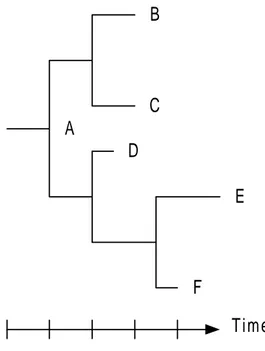
Given a sequence of one protein it is possible to compare it to the sequence of another protein. Theory states that it is possible to measure how closely related two protein sequences are by calculating the number of mutations it takes to transform one protein into the other. Often phylogenetic trees are used to illustrate how closely related the proteins are. A phylogenetic tree is simply a graphical illustration of how a set of proteins relate to each other, based on a distance measure (Figure 1). In the example below the protein that is most related to the root A is D, while E is the protein that is less related with A (it would take the largest number of mutations to go from protein A to E). The example in Figure 1 uses a rooted tree, but usually the tree would be unrooted (the Neighbor-joining method produces unrooted trees while UPGMA produces rooted trees [7]). The reason why unrooted trees are most commonly used is because it is not certain which protein sequence actually is the root.
A B C D E F Time
Figure 1. A phylogenetic tree showing the distances between the 6 protein sequences A-F. The length of a branch between two protein sequences is a measure of the distance between them. The time-axis illustrates that protein mutations happen over time and therefore A would be the ancestor of the whole tree, while E is the most newly found protein.
Artificial neural networks (ANNs) have been used on a variety of different problems. An ANN is presented with an input and then produces an output according to the adjustable weights that connects the input nodes with the output nodes. Essential for an ANN is its ability to learn certain rules by being trained on a set of known
examples and then producing good results when being shown unknown examples. The ANN should both be able to learn and to generalize from the examples presented to it. This ability makes it tempting to try for learning the rules of protein mutations.
2. Thesis Statement
This chapter will present the aim, the problem and the motivation behind the work done in this thesis. The reason for presenting this as early as possible is to make it easier for the reader to agree or disagree with the decisions made.
2.1 Aim
The aim of the work done in this thesis is to predict protein mutations using an artificial neural network. There are two aspects that can be made in this thesis. The first aspect is concerned with computer science and the other is concerned with the biological aspect. The computer science aspect would be to try finding ways to improve the results i.e. finding the neural network that produces the best predictions. On the other hand the biological aspect would examine protein sequences selected on different biological criteria in order to see if it is possible to draw any conclusions about the different results. The aim here is to solve a biological problem using techniques from computer science. That the focus is mainly on the biological aspect does not mean that computer science aspect is uninteresting. As a matter of fact the work done in this thesis is mostly about computer science. However, what is important is the contribution to the biological society. This means that instead of tweaking and comparing ANNs, the ANNs will be kept as simple as necessary. The results of this work will come from comparing actual predicted protein sequences that is based on biological differences e.g. similarity between protein sequences.
2.2 Objectives
In order to predict protein mutations using an artificial neural network a number of objectives exists. Depending on the level of detail a small or large number of
objectives can be found, but the overall objectives can be listed in 3 points. These 3 points are concerned with the following:
• How to select the biological data
There must exist some criteria on which the selection of protein families used for training and testing the ANN is based. The data selected must be of both an easier and a harder nature in order to be able to make some kind of analysis weather the results are good or bad.
• What should the ANN look like
The ANN topology has to be decided. The work in this thesis is not about making the neural networks as good as possible (though it is desirable), rather it is to see if the networks are able to predict protein mutations. The ANNs will have to
perform predictions that are sufficiently good to be able to compare the predictions based on the protein family selection criteria.
• How do we evaluate the predictions
The protein mutation predictions from the neural networks must also be evaluated. The evaluation must be performed using a method that gives acceptable
comparisons i.e. decisions have to be made on how to score the predicted protein sequences.
2.3 Problem Description
As stated, the aim of this work is to predict the protein mutations i.e. from a protein sequence being able to predict what the sequence of a related protein looks like (or possibly what sequences the protein will mutate into). The prediction is done with an artificial neural network (ANN). The assumption here is that the ANN will be able to learn the rules of the mutations from the mutations that takes place in known
phylogenetic trees. The most important difference between the prediction using an ANN and a distance matrix is that the ANN will hold the rules of mutation while the distance matrix holds the data for each and every protein member. Since the distance matrix only contains the score the protein will get for being transformed into another protein (the distance from the closest ancestor) a protein must be in the matrix in order to be investigated. The idea is that the ANN should give information beyond the distance matrix (any protein could be investigated i.e. information about the protein would not have to be stored anywhere) and possibly taking into account additional information e.g. hydrophobicity. The idea is that once a trained ANN is acquired it will be possible to get a prediction of what the sequence after (or before) the presented protein looks like (depending on if the protein is presented at the top or bottom of the network).
Even though this work is novel and nobody (to my knowledge) has tried to predict protein mutations with a neural network, it is not completely ungrounded. Similarity with linguistic approaches to apply grammar with ANN suggests it is possible to perform predictions on protein sequences e.g. Rumelhart and McClelland [2] trained an ANN to learn past tenses of English verbs. The work done in this thesis is not
based on the work by Rumelhart and McClelland; rather it uses their work as an inspiration to the approach for predicting protein mutations.
This work will be concerned with predicting only one mutated version at a time of any protein fed into the ANN (apposed to predicting several mutated protein sequences from a protein sequence). The reason for only predicting one mutated version at a time is that a simple feed-forward ANN only gives one version of the output (1-1 relationship between input-output). When moving upwards in a
phylogenetic tree the ANN would only have to produce one output per protein, but if one moves downwards in the tree several branches would be possible. The idea to train an ANN to predict ancestors of proteins should therefore be easier to do since you are only looking for one answer at a time. However, once there exists a trained ANN that works well with predicting ancestors it should be possible to change direction of the input and output to the ANN, thereby predicting future proteins. As mentioned earlier, if the ANN is simply turned upside-down it will only produce one output when there in fact could be several, but it should be possible to solve this problem also. In this work the problem of predicting future proteins is approached by applying an algorithm (see chapter 4.4.4 Sequence of Proteins) that calculates a path through the phylogenetic tree before training the ANN (from the root downwards).
2.3 Motivation
One problem of interest is to find the ancestor of a protein and another problem is to predict the next generation of proteins. This can be done with the help of a
phylogenetic tree (or at least with the distance matrix underlying the phylogenetic tree). The reason why one would want to find an ancestor to a protein is that nobody
knows what this ancestor looks like (since all life continue to evolve independently) and by finding this ancestor it would be possible to describe what was contained in the creature that e.g. human and pig evolved from. It is also of interest to know what future generations of proteins look like e.g. by knowing what a bacteria that grows immune to penicillin will look like one could experiment with a mutated version of the penicillin. This is all very fancy but the bottom line is that it would be nice to be able to predict proteins.
Imagine you have a phylogenetic tree and a protein that is located somewhere within it. If you move upwards in the tree you will get the ancestor of the protein and if you move downwards you will get the mutated versions of the protein. The problem is that you don’t have the full (or correct) phylogenetic tree over all proteins and you would like to see beyond the root of the tree you have, or beyond the leaves in the tree.
If it is possible to predict the mutation of a protein sequence it could also be possible to predict the mutation of genes. This would take the protein prediction to another level but it would be very interesting to know e.g. what future viruses would look like. The same techniques should be applicable on the prediction of gene mutations,
though. Other fields outside of bioinformatics that the work in this thesis could be of benefit to could be linguistics e.g. by applying grammar to English words (where successful work already has been done). Also, it would be nice to see how the method used in this thesis would perform on translation of words from one language to another (the neural network would have to learn the rules of translation). However, the suspicion is that the rules of translation would be harder to get good results from than the rules of mutation. Basically the method used in this thesis could be of interest
to anyone that has a problem that deals with sequences, predictions and grammar i.e. problems that has to produce an output that is based on an input sequence (by
3. Background
This chapter will describe the domain in which this work will be performed and will serve as a base to the work introduced later. Since this is novel work there will be a brief introduction to the methods used in the approach to solve the problem.
2.1 Problem Domain
The existing method for getting the evolutionary order between proteins is to calculate a distance matrix, containing one distance measure between every pair of proteins, from all proteins you are interested in. From the distance matrix it is then possible to visualize the relatedness between all proteins in the matrix. This is usually done using phylogenetic trees, which is simply a graphical illustration of a tree connecting the participating proteins and where the lengths of the branches relates to the distances between the proteins. To be able to calculate the distance matrix one needs to know the protein sequences in order to run the sequences pair wise through some distance algorithm. One is also bound to work with proteins that are in the matrix and it is appealing to think that it is possible to find the rules for mutation in order to generate new sequences just by applying these rules on one protein sequence. Thus, one should be able to create the same phylogenetic tree as the distance matrix just by applying these rules of mutation.
A B C D E F A 0.00000 0.15236 0.15236 0.13284 0.73648 0.37495 B 0.15236 0.00000 0.00000 0.36453 0.47563 0.41263 C 0.15236 0.13743 0.00000 0.36453 0.47563 0.41263 D 0.13284 0.36453 0.36453 0.00000 0.23943 0.19374 E 0.73648 0.47563 0.47563 0.23943 0.00000 0.12632 F 0.37495 0.41263 0.41263 0.19374 0.12632 0.00000
Table 1. A fictional example used to illustrate the appearance of a distance matrix. A-F are the protein names, and the numbers are the distances between the proteins. The phylogenetic tree of the matrix is seen in Figure 1.
2.2 Artificial Neural Networks
When describing artificial neural networks (ANNs) in this work it will be from the point of view that will make sense regarding the problem at hand. Even though it would be interesting trying to solve the rules of mutation with recurrent networks or even other approaches, here will follow a brief introduction and a description of a feed-forward network.
2.2.1 Introduction to ANN
ANNs works with patterns, getting one pattern as input and producing another pattern as output. These patterns are presented in form of nodes to the ANN and there is a set of adjustable weights that connects all of the input-nodes with all of the output-nodes. In a simple feed-forward version of an ANN the input-nodes and the output-nodes are all directly connected with each other (every input-node is connected to all output-nodes), but it is also possible to have a feed-forward network with several layers of hidden nodes (still with one input-pattern and one output-pattern). An ANN is a learning technique that is trained on a set of known data, and when the weights in the network have been adjusted so it produces the right output (low error), the network hopefully performs well with new data.
2.2.2 ANN and protein sequences
ANNs are inspired by biology and the idea is to simulate the neurons and nerves. When a neuron gets stimulation it sends a voltage through the nerve resulting in another neuron (or group of neurons) on the other side of the nerve to get stimulated, resulting in thoughts and actions. It is from this simple idea that ANNs have evolved, even though it is implemented on a computer and uses the ideas of connectionism, it
is quite tempting to combine with biological problems. The idea that an ANN works with patterns makes it appealing to use with protein sequences since a sequence is a form of pattern consisting of letters representing amino acids. However, there are many ways to represent the input-data to the ANN and this will be discussed in the next section.
2.2.3 A Feed-forward Network
This section will describe a standard feed-forward ANN in order to give some understanding of what type of method is behind the ANNs used in this thesis. The intention with this section is not to fully describe an ANN or ANNs in general, but to give an example of an ANN in order to make it easier to follow the method that is later presented in section 4.2 The Networks. Since it is not certain that the rules for protein mutations are linear separable, an ANN with a hidden layer is used. Therefore, an example of a simple feed-forward network with one hidden layer will be presented on a known problem that is not linear separable, namely the XOR-problem (exclusive or).
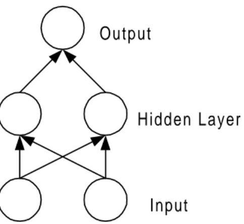
The ANN used for the XOR-problem is found in Figure 2. The XOR-problem uses two binary bits as input from the set {(0,0) (0,1) (1,0) (1,1)} to the network and produces an answer that is either true or false {0,1}. For the input (0,0) and (1,1) the correct output is 0, and for (0,1) and (1,0) the output is 1. Using the 2-bit input representation the XOR-problem cannot be solved without using at least one hidden layer [1].
Input Output
Hidden Layer
Figure 2. The ANN used for the XOR-problem. The input is any binary 2-bit combination. The output is 0 for the patterns {(0,0),(1,1)} and 1 otherwise.
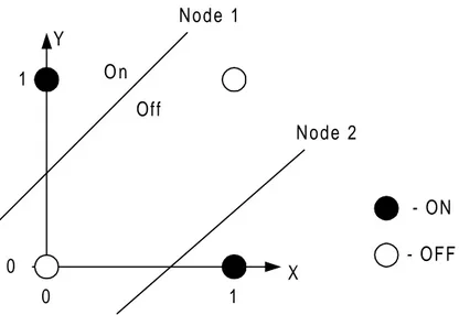
The reason why the network in Figure 2 works can be explained by looking at the two nodes in the hidden layer. Each of the nodes in the hidden layer from Figure 2 can be represented by a line in a 2-dimensional decision space. The line that splits the decision space turns everything on, on one side of the line and off on the other side. From Figure 3 it is easy to see that it takes two lines in order to be able to turn on only the (0,1) and the (1,0) positions, and hence the need for a hidden layer. The lines in the decision space are drawn from the input and the weights to the two nodes in the hidden layer. When the ANN is trained on the XOR-problem it is actually the weights that determine the positions and angles of the lines that are adjusted until a setup like in Figure 3 is achieved.
0 0 1 1 X Y Node 1 Node 2 O n Off - ON - OFF
Figure 3. Decision space for the XOR-problem. Each line in the decision space acts like a border in where one side is always on and the other is always off. The lines are drawn from the inputs and weights to the two hidden nodes. It takes two lines to separate the decision space so that positions (0,1) and (1,0) are turned on while (0,0) and (1,1) are turned off.
When training the networks in this thesis, standard back propagation for a multi-layered network is used (the generalized delta rule [1]). For a complete description of how networks are trained and how errors are back propagated a good description can be found in the work by Rumelhart et. al. [1]. In this section a clarification has been made, why the prediction network uses multiple layers by comparing to the XOR-problem. The motivation of network topology is important since this is novel work (to our knowledge). The detail of how an ANN works is well documented in other work, and also the focus of this work is on the biological side.
2.3 Distance Matrix
A distance matrix contains the distances between all protein members in the matrix. The distance matrix works by comparing two aligned protein sequences at a time at
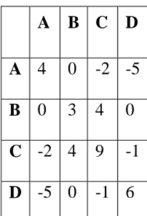
each and every amino acid position. At every amino acid position (whether it is a match or a mismatch) a score is looked up for the amino acid substitution (amino acids can also be substituted with themselves e.g. A is substituted with A). The sum of all substitution-scores between the protein sequences will then give a measure of how closely related the proteins are. A toy example of how to calculate the distances between two short protein sequences can be found in Table 2 and Table 3. Table 2 holds a table of how to score the individual substitutions that is later used to score the whole protein sequence (Table 3). The sequences in Table 3 shows that even if there is only a 50% match between the sequences the score will still be positive (due to the scoring for the individual sequences).
A B C D A 4 0 -2 -5 B 0 3 4 0 C -2 4 9 -1 D -5 0 -1 6
Table 2. The substitution-scoring matrix used to look up the individual substitution penalties or rewards. This table shows if a substitution is to be considered good or bad.
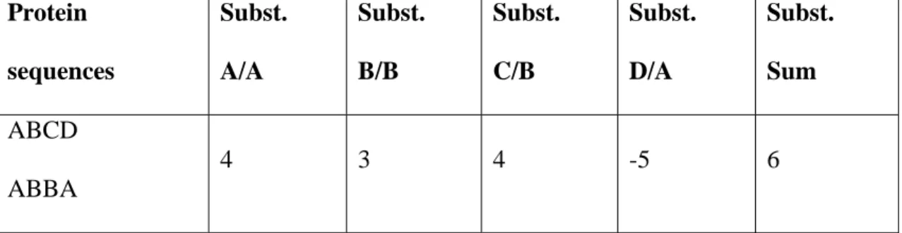
Two different methods have been used in this work in order to calculate the distances between protein sequences and their amino acids, namely the Blosum matrix and the Phylips protdist program [9] (using the Dayhoff PAM matrix). It is suggested by Geoffrey J. Barton [6] that the BLOSUM62 matrix is commonly most effective. Protein sequences Subst. A/A Subst. B/B Subst. C/B Subst. D/A Subst. Sum ABCD ABBA 4 3 4 -5 6
Table 3. This table shows how to score the distance between two protein sequences. There are four substitutions between the sequences and the final score is summed up at the end (Sum=6).
4. Method
This chapter will explain the methodology used in this work for trying to solve the problem of predicting protein mutations. The methodology consists of several steps and therefore this chapter starts with an overview to connect the different subparts. The setup and the subparts will then be explained.
4.1 Overview
There exists a biological problem of finding the rules of mutation for proteins. This problem will be approached with techniques from computer science and the first objective would be to collect real data to work with. In order to be able to train the ANN there must also be a decision of how to represent the protein sequence data and the topology of the ANN.
For collecting data, databases available on the Internet will be used e.g. Pfam [3] or BLOCKS [4]. In order to calculate a phylogenetic tree Protdist will be used, but a phylogenetic tree is not really necessary (except for visualization purposes) since all information that is needed to train the ANN is already within the distance matrix. The distance matrix will be the foundation for training and testing the ANN. To calculate the distance matrix the Phylip web-service will be used [9].
The idea behind the protein mutation prediction problem is that it will be possible to predict protein mutations from one generation to another. The ideal situation would be to have equally spaced distances between the protein sequences that are used for training the ANN. That is, for every pair of protein sequences used for training the ANN the distance between then should be the same as in all other sequence pairs.
However, it is not the case that the protein sequences in the databases available will contain equally distanced protein sequences i.e. the data available will have different length between the protein mutations. Also, starting at one protein sequence, it is not likely that every mutation that follow from that sequence will be stored in a database. What will be found in the databases are more or less closely related proteins. It is likely that some sequences are missing from the database that in fact exists (or have existed) in the nature. Missing proteins makes it hard to do a fair comparison of the predicted protein and the actual protein, especially if the actual protein might be missing. The ideal setup of the data used would be to have access to all protein sequences in a protein family, evenly spaced in the sense of evolutionary time i.e. sequences that are as closely related as possible.
The method for collecting data to this project will be to first of all decide on a family of proteins. It is possible to decide on one protein and then to perform a homology search where all proteins above a chosen threshold will be used. This would guarantee some degree of similarity between the protein sequences. Since this project will use an ANN to perform the protein mutation predictions it is required that the protein sequences are aligned in order to train the network. In order to get multiple aligned sequences, databases such as the BLOCKS database [4] or Pfam [3] will be used. In this way the data will be set up in a format that will be suitable for training and testing an ANN.
Once there exists a set of aligned protein sequences the order in which they have evolved must be decided i.e. the relational distances between the protein sequences must be decided. This will be done by calculating a distance matrix from the whole
set of aligned protein sequences. It is intended to use the Protdist program found on the Internet in order to do this.
Having the distance matrix it is possible to calculate a single sequence from a protein in the matrix to its ancestors. This way a single sequence will be created from one protein to another making it possible to create a training-set and a test-set for the ANN. The ANN will be trained using the training-set until the protein mutations are classified correctly (with some degree of error-marginal of course). Once the ANN is trained it must be tested on data that is new to the ANN (the test-set) in order to see if it is possible for the ANN to actually learn the rules of mutation (the mutational grammar).
4.2 The Networks
In order to solve the protein mutation prediction problem two different ANNs has been used. One ANN is used to predict the protein mutations as was intended for solving this problem. An additional ANN has also been used in order to compress the amino acid representation to the prediction network.
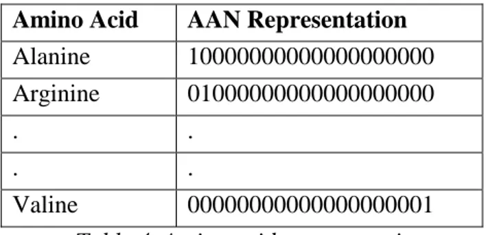
Since there are 20 different amino acids there would have to be 20 input nodes to the ANN to represent just one amino acid (Table 1) i.e. an ANN that read 100 amino acids at a time would have to have 2000 input nodes. Furthermore, each node is connected to the next layer of nodes with weights. This means that in an ANN with one hidden layer of 100 nodes (a 2000-100-2000 topology) there would be 400,000 weights that would have to be adjusted each epoch the network is trained. In order to keep the number of input and output nodes down in the prediction network a different
ANN, an auto associative network (AAN), will be used. The idea with this network is that it should learn to represent the 20 different amino acids with less than 20 nodes per amino acid e.g. the 20 nodes coding for Alanine will be represented with only 3 nodes, thus reducing the number of input nodes in the previous example from 2000 to only 300. The reduction of input nodes and output nodes makes the network topology smaller and greatly reduces the number of weights. For comparison the 2000-100-2000 topology network with 400,000 weights would correspond to a 300-15-300 network with only 9000 weights. A more reasonable topology might be 300-100-300, resulting in 60,000 weights (then the corresponding uncompressed 2000-666-2000 network would have 2,664,000 weights).
Amino Acid AAN Representation
Alanine 10000000000000000000 Arginine 01000000000000000000 . .
. .
Valine 00000000000000000001
Table 4. Amino acid representation.
It is also possible to use additional information about the amino acids and to encode it into the network e.g. physico-chemical information (hydrophobicity, weight etc.). Uncompressed, this would increase the number of input nodes coding for an amino acid but this information could also be included into the compressed version of the representation.
4.2.1 Compression ANN
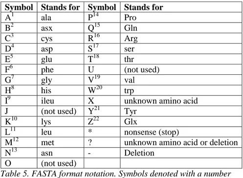
The topology of the auto associative network (AAN) will be as in figure 1, with 22 input nodes, 22 output nodes and 3 nodes in the hidden layer. The reason why there are 22 nodes in the input and output layer is that the representation is based on the notation used in the FASTA format. The ultimate compression would also be to use only one hidden node, but this is not the focus in this work (since the focus is to predict protein mutations without adding further noise).
The FASTA format notation uses 26 different symbols in its representation (Table 5). To represent amino acids in this work the symbols A-I, K-N, P-T, V,W,Y and Z are used (they are marked with their respective numbers in Table 5). Even though, all protein sequences that are used are in FASTA format and therefore uses 26 different symbols to be represented, 22 symbols should be enough in this work. The reason why 22 symbols are enough is because only a part of the multiple alignment is used with the networks (like a window). There are two extra symbols in the representation used: B and Z (where B denotes either D or N, and Z denotes E or G).
Symbol Stands for Symbol Stands for A1 ala P14 Pro B2 asx Q15 Gln C3 cys R16 Arg D4 asp S17 ser E5 glu T18 thr
F6 phe U (not used)
G7 gly V19 val
H8 his W20 trp
I9 ileu X unknown amino acid
J (not used) Y21 Tyr
K10 lys Z22 Glx
L11 leu * nonsense (stop)
M12 met ? unknown amino acid or deletion
N13 asn - Deletion
O (not used)
Table 5. FASTA format notation. Symbols denoted with a number shows that they are being used in the auto associative network representation.
The AAN will have to be trained to correctly identify all 22 amino acid representations and when this is done each amino acid would have a unique
compressed representation to be used in the prediction network. Since the objectives for the AAN is to correctly encode and decode the 22 different amino acids symbols it will just have to serve as a memory in the first stage (encoding). In the stage of
decoding, however, it is important that the output from the prediction network is not oversensitive to small fluctuations in the compressed representation i.e. the resulting protein sequence should not be altered by the decoding process (see discussion).
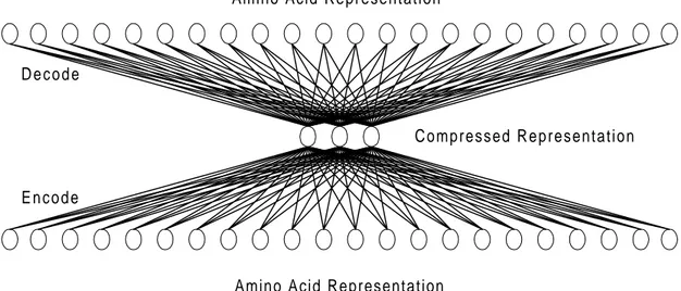
Amino Acid Representation Amino Acid Representation´
E n c o d e D e c o d e
Compressed Representation
Figure 4. The Auto Associative Network (AAN) for compressing amino acid
representation. The input and output is either of the amino acid representations found in Table 4. The compressed representation (3 nodes) can then be used in the
prediction network instead of using the normal representation (22 nodes).
The evaluation of the AAN is straightforward since the network is auto associative. The whole idea is for the network to produce the same output as input. However, the AAN must still be able to cope with decoding compressed nodes with small variations and this must also be evaluated.
4.2.2 Prediction ANN
The prediction network will be a standard feed-forward network with three layers (input-hidden-output). Based on Rumelharts work [2] it might be sufficient with only two layers (input-output), but the assumption in this work is that there is a need for a hidden layer. This assumption is based on the uncertainty weather the problem is linear separable or not (better to be safe than sorry). As mentioned before similar approaches have been successfully performed within the linguistic community (to
successfully used an ANN without any hidden layers and the similarity of this problem should work with the current setup (3-layers).
The idea with the prediction network is that when it is trained one can use any protein sequence as input and the network will translate it into the predicted mutated version. The prediction network will hold the rules for mutation learned from the data it has been trained on i.e. if the predictions are correct. The prediction network holding the rules of mutation will give the input sequence a transformation/mapping to the predicted/mutated sequence.
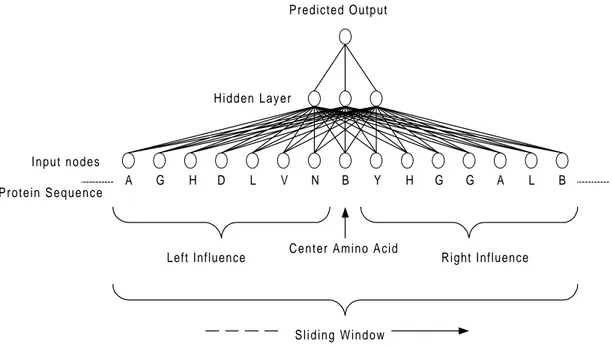
The prediction network will have a fixed size window of input nodes. The network uses the same topology of the network as the compression network in Figure 4, but with a different number of nodes. Baring in mind that the technique of looking at a block of amino acids at a time later can be transformed into a sliding window approach (Figure 5). A sliding window would look at a block (window) of amino acids at a time, starting at the beginning of the protein sequence sliding towards the end of the sequence, producing only one output per step. A sliding window would only try to predict one amino acid at a time (the center amino acid), but would take into account the adjacent amino acids (left and right influence in Figure 5). While the window is moving along the protein sequence, predicting mutations in each step, it would hence produce the mutated version of the protein sequence along its way. What makes the sliding window technique different from the block prediction network is that the sliding window network will hold more information. The reason why the sliding window network holds more information is that the left and right influence is used in the prediction of every single amino acid. If a block is predicted with both the
block prediction network and the sliding window network, the sliding window will give extra information in the beginning and the end of the sequence. The left and right influence sees beyond the start and end of the predicted block giving that additional information i.e. if the block is not exactly the whole protein sequence).
B
A G H D L V N Y H G G A L B
Protein Sequence
Predicted Output
Hidden Layer
Center Amino Acid
Left Influence Right Influence
Sliding Window Input nodes
Figure 5. The sliding window technique, showing prediction of one amino acid at a time. This is done considering the amino acid at the center of the input, but also under influence by the adjacent amino acids.
The block prediction network used in this work will, unlike the sliding window approach, attempt to predict a whole sequence block at a time. The block approach is used because the protein sequence data can then be chosen to include only the
selected symbols used in the representation (Table 5). The first thing would be to see if it is possible to predict blocks of amino acids like it is done in this work. If a sliding window technique were to be used to predict the protein mutations from the
alignments (in FASTA format) a decision would have to be made about how to handle e.g. the insertions.
4.2.3 Both Networks Working Together
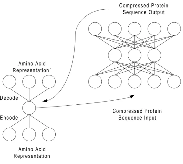
Both the auto associative network (AAN) and the prediction network will work together while predicting protein mutations. The AAN will serve as an encoder to compress the data input to the prediction network and as a decoder to make the output of the prediction network readable again (Figure 6 illustrates this).
The AAN will be trained separately and only at one time until it successfully encodes and decodes the amino acids (using the representation in Table 4). Once the AAN is working successfully it is possible to concentrate on the prediction network. The input to the prediction network is in form of a translated sequence block where each amino acid is represented by 3 nodes. The AAN is now simply used to compress each amino acid in the sequence block, for each amino acid putting the contents of the hidden nodes into the input nodes of the prediction network. The prediction network can now be trained or tested on its input, generating a prediction of a protein sequence
mutation. In order to be able to understand the output of the prediction network the output must be translated back into a FASTA-format sequence. This is done by feeding to prediction output in pairs of 3, into the hidden layer of the AAN. The AAN will then decode the input to the hidden nodes while producing an output that can be translated from Table 4 and into FASTA format by Table 5.
Amino Acid Representation Amino Acid Representation´ E n c o d e D e c o d e Compressed Protein Sequence Input Compressed Protein Sequence Output
Figure 6. The complete system with both AAN and the prediction network.
4.3 Collecting Data
The first procedural step of predicting protein mutations is to collect data. The data selected will be what the prediction network later has to learn its rules of mutation from. The natural choice of data is to choose a whole protein family since the protein sequences within a family are somewhat similar (close evolutionary distances). The goal with the data is to find the order of evolutionary mutations so that the prediction network can learn its rules.
When choosing a protein family one can choose from existing protein databases on the web. This project will collect the protein sequences from Pfam [3] and the
4.3.1 Pfam
Pfam has a service that makes it possible to browse the protein families. For each protein family there is also additional information such as the number of protein members in the family, average length, a measure of similarity between the protein sequences and a short description (an excerpt from Pfam can be found in Table 6).
Name No. seed No. full Average Length Average %id Structure Description 14-3-3 16 119 212.3 69 14-3-3 proteins actin 24 430 308.1 74 2btf Actin
cytochrome_c 44 285 93.1 28 1cry Cytochrome c
S_T_dehydratase 32 121 297.7 26
Pyridoxal-phosphate
dependent enzymes
sugar_tr 50 444 436.9 16
Sugar (and other) transporter
Table 6. Excerpt from the Browse Pfam service. The seed column shows the number of hand edited multiple aligned sequences representing the domain. The full column shows the number of sequences that was found using an automatic hidden markov model. Average %id is the similarity between all family sequences en percent.
Pfam makes it easy to maneuver between the different families in the database and if further information is needed about a specific family there are links directly to the Prosite database [5]. Prosite contains information about proteins and protein families and gives a good description of the protein, or family one is interested in. Also, in Prosite vital information about proteins can be found e.g. active sites or patterns.
4.3.2 The BLOCKS database
The Blocks database [4] is very appealing to use in this work, since the method for predicting protein mutations in this work already has been stated as using blocks of sequences. The Blocks database contains multiple aligned blocks of protein sequences that can be attained e.g. by query the blocks database for a specific protein family (Table 7).
ID ACTIN; BLOCK
AC PR00190A; distance from previous block=(8,30) DE Actin signature
BL adapted; width=10; seqs=140; 99.5%=642; strength=1320
ACT2_NAEFO (22) APGAVFPSII 60 ACT1_ECHGR (26) SPRAVFPSLV 53 ACTD_PHYPO (23) TPRAMFPSIV 77 ACT1_PEA (27) DARAVFPSIV 48 ACT1_SOYBN (29) PPRAVFPNIV 54 ACT2_PEA (27) DARAVFPSIV 48 GIAACTI (26) APRAVFPTVV 64 ACTM_STYPL (30) PPRAVFPLTV 77
Table 7. Excerpt from a search in the Blocks database. The columns show the name of the protein, the position of the first residue in the segment, the block segment and the weight. The weight is a measure of how similar the segment is compared to the other segments in the block (weight=100, means maximum dissimilarity).
It is also possible to combine the Pfam results with the Blocks service. This can be done by choosing a protein family from Pfam, letting Pfam perform the multiple alignment, and then use the Blocks multiple alignment processor service to extract the blocks.
4.4 Preparing Data
Once a protein family has been chosen a number of steps must be taken in order to be able to use the proteins with the prediction network.
4.4.1 Multiple Alignment
All the sequences in the protein family must be aligned to make it possible to compare the amino acids at their specific positions in the protein sequence. If two evolutionary adjacent protein sequences were to be aligned it would be possible to detect the amino acid mutations at every position. Even if the protein sequences are of different length the multiple alignment makes sure that all aligned sequences will be of the same length (by using inserts/deletes). It is possible to perform a multiple alignment by using a scoring method that gives penalties for inserts/deletes and rewards amino acid matches. By using a scoring method like this the cheapest combination of
inserts/deletes would give the best alignment. There are a number of services on the Internet that provides multiple alignment of protein sequences (e.g. ClustalW [8]) but in this work the alignment from Pfam [3] or the Blocks database [4] is used. An alignment from the Blocks database differs some compared to the other methods in that only a part of the complete protein sequence is aligned and that no inserts/deletes are used. The fact that the alignments from the Blocks database only contains pure
amino acids in the regions that is essential for the protein family makes it very useful to use in this work.
4.4.2 Block Format
Once a multiple alignment is attained from the sequences in the chosen protein family, a block (or a window) of sequences would have to be cut out. The size of this window relates directly to the number of the chosen input nodes in the prediction network. The idea behind this is to be able to use the same network topology for the prediction network regardless of what family is under investigation, making it possible to directly compare the different networks (trained on different protein families) with each other. This block of sequences is cut out manually from the multiple alignments and could be taken from anywhere within the alignment provided by the Blocks database.
4.4.3 Distance Matrix
The step that must be taken after there exists a number of aligned and unsorted protein sequences is to calculate the evolutionary distances between the proteins. This is done using the Protdist program in the set of tools provided by Phylip [9] (Dayhoff PAM matrix). Protdist generates a distance matrix that contain a measure of the distances between each and every protein sequence. The distances in the matrix are related to the evolutionary distances between the proteins and can be used to calculate the order from which the proteins have evolved.
4.4.4 Sequence of Proteins
Once a distance matrix is attained the job is to create data that makes it possible to train and test the prediction network. This is simply done by an algorithm that chooses one of the proteins in the distance matrix that are closest related (and the distance isn’t zero). Starting with this selected root, the algorithm creates an evolutionary sequence from the selected protein (always choosing the most closely related protein without creating a loop). By creating a sequence of proteins (sequences) it may be possible not to get all of the family members in the data-set (unless several evolutionary sequences of proteins are created). In this work one evolutionary sequence will be sufficient (it seams sufficient with one evolutionary sequence of proteins to pick up the rules of mutation in a protein family). By applying the algorithm of selecting a sequence of proteins on the toy example in Table 1, the root selected would be E since the distance between E-F is the shortest in the matrix. With E as the root in the phylogenetic tree the sequence of proteins would be as illustrated in Table 8. Further illustration can be found by comparing the sequence in Table 8 with the phylogenetic tree in Figure 1. By comparing Table 8 with the tree in Figure 1, it is possible to see that with E as the root, the algorithm will create a sequence of proteins that follows the shortest
distances. Also, it is possible to see that protein C is left out, since the distance between B-C is zero.
Sequence Order
Protein #1 Protein #2 Distance
1 E F 0.12632 2 F D 0.19374 3 D A 0.13284 4 A B 0.15236
Table 8. The order of protein sequences calculated by the sequence-algorithm, used on the matrix in Table 1. The resulting sequence is the result of choosing E as the root in the phylogenetic tree.
4.4.5 Choose Test-set & Training-set
From the evolutionary sequence of proteins it is now possible to create a test-set and a training-set for the prediction network. This is done by choosing about 20% of protein sequences to be in the test-set and the rest of the sequences will be used for training the prediction network. When choosing a test-set the sequences are selected so they are evenly spaced over the whole evolutionary sequence, avoiding adjacent protein sequences to be selected. This is done in order to try to even out the gaps in the evolutionary distances that will be the result when picking out sequences from the distance matrix.
4.5 Train ANN
The training of the prediction network will be done using the calculated training-set from the data collected. The attempt will be to predict, from the ancestor protein sequence, the succeeding protein sequence. In Figure 7 below the fist ancestor would
be ADH1_HORVU and the predicted protein should be ADH1_PEA i.e. sequence number 1 is presented to the prediction network and sequence number 2 should be the prediction output. If the sequence of ADH1_PEA is presented to the prediction network (the ancestor) then the sequence of ADH1_ARATH should be the predicted output (and so on).
Protein Distance --- ---0.00000 0.06101 0.06227 0.10060 0.10195 Ancestors Mutations 1.ADH1_HORVU: EVRVKILFTSLCHTDVY 2.ADH1_PEA : EVRLKILFTSLCHTDVY 3.ADH1_ARATH: EVRIKILFTSLCHTDVY 4.ADH1_PENAM: EVRVKILYTSLCHTDVY 5.ADH1_SOLTU: EVRLKILYTSLCHTDVY
Figure 7. Prediction of ancestor protein (data from BLOCKS [4] and Protdist [9]).
4.6 Evaluate ANN
The prediction network will be evaluated using the test set (not the same sequences used for training) of the proteins calculated with the distance matrix. Since the proteins have been ordered (based on their evolutionary distances from the distance matrix) and a test-set has been selected, the first step of evaluation is straightforward. By Remembering where the sequences in the test-set actually should be located in the complete sequence of protein sequences (section 4.4.4) one would expect the test-sequence to be predicted from its immediate ancestor. E.g. if test-sequence number 2 (ADH1_PEA) in Table 2 was in the test-set (and not in the training-set), one would expect the prediction network to produce this sequence as output when sequence number 1 is fed into the prediction network.
4.6.1 Using the Test-set
As mentioned above the expected output from the prediction network is known in advance when using the test-set as input to the network. Also, it is known that there do not exist any adjacent protein sequences in the test-set. This way it is possible to directly compare the predicted output with the expected output.
The sequence that serves as the ancestor for the prediction must first be translated in the compression network (section 4.2.3) before it is shown to the prediction network. The prediction network then works by applying what it has learned from the training-set onto the protein sequence, resulting in a new predicted successor. The newly predicted protein sequence is still in a compressed format so it’s not very easy to interpret and therefore some additional steps must be taken before the whole prediction procedure is complete.
4.6.2 Decode Prediction
When the prediction network has produced a new protein sequence it must be
decoded by the AAN in order to make the sequence readable (even more important if extended information would be encoded in the compressed representation). The decoding process is not as trivial as the encoding process. This is because the output from the prediction network (3 nodes represent one amino acid) does not exactly agree with the encoding part of the compression network (Table 9) i.e. both the prediction network and hence the AAN will have some degree of error at their output. The aim of the prediction network is to predict protein mutations while being as close as possible to the exact compressed amino acid representation.
By using an AAN to encode and decode the amino acid representations it is possible to introduce errors in the predictions. This is especially true if the prediction network has problems predicting nodes that are similar to the exact compressed amino acid representation. However, it is the belief that the prediction network will make predictions that are close enough to the expected results and therefore produce the same predictions as without the compression network. The use of a compression network could also help to improve the predictions if additional information is used in the AAN e.g. hydrophobicity and weight.
The output from the compression network should be in the binary form shown in Table 4, but the output is actually not this clear (so a filter is used).
Node 1 Node 2 Node 3
Exact compressed representation 0.626 0.002 0.775 Prediction output representation 0.632 0.004 0.774
Table 9. The output from the prediction network does not exactly match the representation used for encoding an amino acid. The exact compressed
representation shows the values of the nodes used to encode the amino acid Alanine. The prediction output representation shows the values of the nodes for one amino acid (Alanine) at the output from the prediction network.
4.6.3 Filter the Result
In order to automate the prediction procedure as much as possible and to clean up the compression network output a filter is used on the output from the compression network. The task of the filter is simply to decide on which representation of amino acids (Table 4) that gives the best match. The filter works by selecting the node with the highest activation turning this node on, while turning off all other nodes (Table 10). If there are two (or more) nodes that have a high activation the filter will still select the node with the highest activation. If more than one node has equally the highest activation, the first (leftmost) node will be selected as being the correct output (this should almost never happen). In Table 10 below is an example of how the filter works. The compression network output is not exactly correct since the prediction output representation from Table 9 is used as input to the compression network. The filter then selects node 1 as the highest activated node, setting this node to 1, while all other nodes are set to 0. The resulting amino acid con now be looked up in Table 4 and translated to its symbol in FASTA format (Table 5).
Node 1 2 3 4 5 6 7 8 9 10 11 COMPRESSION NETWORK OUTPUT 0.900 0 0.041 0 0.039 0 0 0 0 0 0 ACTUAL AMINO ACID REPRESENTATION 1 0 0 0 0 0 0 0 0 0 0 Node 12 13 14 15 16 17 18 19 20 21 22 COMPRESSION NETWORK OUTPUT 0 0.061 0 0 0 0.042 0 0 0 0 0.053 ACTUAL AMINO ACID REPRESENTATION 0 0 0 0 0 0 0 0 0 0 0
Table 10. This table shows the actual output from the compression network (Alanine, see Table 4) and the desired output. The task of the filter is to translate the
compression network output into the actual amino acid representation. This is simply done by choosing the highest activation of the compression network output and setting this bit to 1 while the others are set to 0.
4.6.4 Translation into Protein Sequence
The final step in the prediction procedure is to translate the amino acid representation back into FASTA format. The translation is done one amino acid at a time, forming the complete protein sequence block. This is done in order to make it easy to compare the input sequence with the predicted (output) sequence. Once the predicted sequence is in FASTA format additional tools can be applied to both the input sequence and the
predicted sequence e.g. using ClustalW [8] to calculate a similarity-score between the sequences.
4.7 Chapter summary
The method used in this work can be described in 3 overall steps: Collecting data
- Multiple Alignment, from Blocks or Pfam - Calculate Distance Matrix (DM), from Protdist Train ANN
- Using training set from DM Evaluate ANN
- Using test set from DM
Each step holds in turn several practical moments that must be performed in order to get a procedural way of working while using the results from one step in the
following step.
A more detailed (or practical) description of the prediction method can be in place. This description is the result of running different programs and tools that is necessary to perform in order to produce the required results. An overview of the procedure that is used in this work can be put like this:
1. Choose protein family (Browse Pfam or BLOCKS database) 2. Multiple alignment in FASTA format (Pfam)
3. Cut out a block of the alignment 4. Calculate Distance Matrix (Phylip)
5. Make a sequence of proteins from DM (auto.) 6. Make test & training set from sequence
7. Translate test & training set into compressed representation (auto.) 8. Train Prediction ANN with training set (auto.)
9. Test Prediction ANN with test set (auto.) 10. Decode Prediction ANN output (auto.)
11. Filter Decode ANN result to select highest activation (auto.) 12. Translate Filter output into protein sequence (auto.)
The lines that are marked with “auto.” indicate that special purpose software has been implemented to be able to perform these actions automatically.
5. Results
In this chapter the results from using the neural network method (described in
previous chapter) on different protein families are presented. First, a description of the logics behind the experiments will be explained. Secondly, there will be a brief
description of the proteins used in the experiments to give some understanding of why these families have been chosen. The results will be presented in such a way that it is possible to make it possible to compare how well the prediction networks perform on the different families. In the end of this chapter there is also a demonstration of predicting mutations using the sliding window technique.
5.1 The Experiments
The idea behind the experiments is to keep the prediction network topologies the same and see how the networks will perform on the different protein families. It is believed that better results could be attained using a different network topology or even when using one specialized prediction network topology per protein family. However, what is of interest here is not how good results it is possible to obtain, rather that it is possible to get results i.e. it is assumed that there exists a functional relationship between protein mutations. By keeping the network topologies the same for all experiments it is possible to compare the results between the different protein families (instead of comparing results between the different networks). Additional experiments have also been performed (using the sliding window technique) in order to be able to compare with the results of a different method using another network topology.
5.2 Protein Families
The main criteria for choosing a protein family is the similarity between the
sequences of all protein family members. As described in the previous chapter this is done by first selecting a family in Pfam (browse Pfam, Average%id). To learn more about the protein family the Prosite documentation [5] is used to see what is
mentioned about how well conserved the family is.
The protein families chosen for these experiments are the following:
• 14-3-3 • Actin
• Cytochrome C • S T Dehydratase • Sugar tr
The 14-3-3 and the Action families are well conserved while the others are not (as seen in table 3). The Sugar transport family is the family less conserved according to the numbers used from Pfam (e.g. see Table 13).
5.3 Scoring
The predictions of the protein sequences from the prediction networks will not always be exactly correct i.e. the predicted amino acid will not always be the same as the expected amino acid. As long as the prediction of an amino acid is correct there is not much to argue about, but when the prediction is incorrect it does not necessarily have to be a bad thing (some amino acids can substitute for each other meaning that the protein sequences would be different but would still have the same functionality). In
order to take this into account when scoring the predicted protein sequences different blosum matrixes is used with help from the ClustalW sequence alignment scoring [8].
In Table 11 you will find the method behind the mismatch scoring. In all predictions where there is a mismatch of the predicted and the expected amino acid the Blosum matrix is used to give a penalty or reward. The individual mismatch scores are then summed up and a final mismatch score for the whole protein sequence is presented. As seen in the examples in Table 11 all mismatches do not necessarily have to be bad. Looking at the 3 first amino acids in the 14-3-3 family (Table 11) the first amino acid is a match (R) and everything is fine. The second amino acid is an E while it was expected to get a D, but looking up the penalty for the E/D substitution in the blosum matrix shows that this actually is a good substitution (+2). Similar with the third amino acid where we have to look up the R/Q substitution and find that also this substitution is somewhat positive (+1). In Table 11 below are examples of two fully predicted protein sequences and the scoring from the blosum60 matrix.
Family Name 14-3-3 Sugar_tr
Input Sequence RDEYVYKAKLAEQ VLVGKILAGVGIG
Predicted Output RERLVYWZKLAEQ YSVGHIIAGVGIG
Expected Output RDQYVYMAKLAEQ LVAGRTVAGVGIG
Match/Mismatch +---++--+++++ ---+---++++++ Y/L=-1 E/D=2 S/V=-2 R/Q=1 V/A=0 L/Y=-1 H/R=0 W/M=-1 I/T=-1 Blosum Scoring Z/A=-1 I/V=3
Mismatch Score Sum: 0 Sum: -1
Table 11. An excerpt from the actual sequence predictions of the families 14-3-3 and Sugar transport. The table shows the input sequence to the prediction network, the actual predicted sequence and the expected output sequence (from the calculated evolutionary sequence). The Blosum scoring shows the rewards/penalties for the mismatches at each amino acid position (from the Blosum60 matrix). Finally the rewards/penalties are summed up and the final mismatch score is calculated.
5.4 Prediction Results
This chapter holds all the final results for all predictions. To get the results presented in this chapter one ANN has been trained on each protein family (except for the generalization example). This way each prediction network should be specialized on their respective family. In the generalization example, one prediction network has
been trained on all the protein families in order to see if it is possible for the network to generalize between different protein families. Additional results for using the sliding window approach are presented at the end of this section.
Below there is a description of the results from the different protein families using a specialized prediction network followed by the results using the generalized
prediction network and finally the results for the sliding window technique.
5.4.1 Specialized Prediction Network
In order to get the following results one prediction network with a 39-20-39 topology has been used on each and every protein family i.e. one specialized network per family that handles a protein sequence block of length 13. The lowest training error was found around 20000 training epochs, and this was the case for almost all
prediction networks. In Table 12 below the training errors for the different networks can be found and also the number of examples used for training and testing each family.
Protein Family NrTrain NrTest Error1000 Error10000 Error20000 Error30000
14-3-3 54 13 0.262445 0.263347 0.190700 0.251205 Actin 68 16 0.481293 0.289271 0.250689 0.356522 cytochrome_c 212 52 4.928870 5.285871 5.285876 5.010879
S_T_dehydratase 15 4 0.006438 0.000421 0.000128 0.000074 Sugar_tr 76 18 2.993614 3.031121 2.426962 2.756046
Table 12. The fist column shows the name of the protein family. The second and third column shows the number of examples used for training and testing. The other
columns show the network training error after 1000, 10000, 20000 and 30000 epochs respectively.
By using the ClustalW [8] service to calculate the Blossom score for the prediction mismatches it is now possible to give a score for the predicted protein sequences that is fairer than to simply count the number of matches. The scores for the prediction of sequence blocks, using the 39-20-39 network topology can be found in Table 13.
Name Average%id NrTest AvgTrueHits Avg. NoMatch Al.Score
14-3-3 69 13 10.69 0.0769
Actin 74 16 8.06 2.06
Cytochrome_c 28 52 7.13 -1.1
S_T_dehydratas 26 4 5.25 -4.5
Sugar_tr 16 18 5.72 0.83
Table 13. The final results for the block prediction method. The first column shows the name of the protein family. The second column holds a measure in percent that shows how similar to each other all protein sequences in a family are (from Pfam). The NrTest column shows how many sequences (blocks) were used to test the
prediction network (20% of all family members used). AvgTrueHits shows the average number of amino acid in a block that was correctly predicted (max number of matches for a block is 13). The final column shows the average score for all mismatched amino acids (calculated with ClustalW Blosum scoring).
5.4.2 Generalized Prediction Network
The generalized prediction network is an experiment to see if it is possible for a prediction network to learn to predict correct results over several protein families. The generalization network was trained on all protein families except for the Cytochrome
C family. The idea is to see if the generalized network then will be able to produce the same results on the Cytochrome C family as the specialized prediction network. The final results for the generalization prediction network can be found in Table 14 below.
Name Average%id NrTest AvgTrueHits Avg. NoMatch Al.Score
14-3-3 69 13 10.69 17
Actin 74 16 10.5 20.63
Cytochrome_c 28 52 0.67 -1.98
S_T_dehydratas 26 4 2.75 -12.25
Sugar_tr 16 18 6.5 49.17
Table 14. This table contains the results for the generalized prediction network. The columns are calculated exactly as in Table 13 with the only difference that in this table only one prediction network was used on all protein families (except for the cytochrome C family).
The generalization network has the same topology as all the specialized networks (39-20-39). In this way it is possible to directly compare the results.
5.4.3 Sliding Window Results
Using the sliding window technique was done as an additional experiment in order to compare how a different approach (and network topology) would perform on the protein families. Only two protein families were used for these experiments since the main work was done on the block prediction method.