Evaluation of a method for identifying timing models

(1)

1

Evaluation of a method for identifying timing models

MASTERS IN SOFTWARE ENGINEERING 30 CREDITS, ADVANCED LEVEL

Author: Lidia Tesfazghi Kahsu

14th June 2012

Supervisor/Examiner: Björn Lisper

bjorn.lisper@mdh.se

(2)

2

ABSTRACT

In today’s world, embedded systems which have very large and highly configurable software systems, consisting of hundreds of tasks with huge lines of code and mostly with real-time constraints, has replaced the traditional systems. Generally in real-time systems, the WCET of a program is a crucial component, which is the longest execution time of a specified task. WCET is determined by WCET analysis techniques and the values produced should be tight and safe to ensure the proper timing behavior of a real-time system. Static WCET is one of the techniques to compute the upper bounds of the execution time of programs, without actually executing the programs but relying on mathematical models of the software and the hardware involved.

Mathematical models can be used to generate timing estimations on source code level when the hardware is not yet fully accessible or the code is not yet ready to compile. In this thesis, the methods used to build timing models developed by WCET group in MDH have been assessed by evaluating the accuracy of the resulting timing models for a number of combinations of hardware architecture. Furthermore, the timing model identification is extended for various hardware platforms, like advanced architecture with cache and pipeline and also included floating-point instructions by selecting benchmarks that uses floating-points as well.

Keywords: Real-time systems, WCET analysis, simulation, Early timing analysis, SimpleScalar, SWEET, Linear timing models

(3)

3

ACRONYMS

(BCET): Best-Case Execution Time (HW): Hardware

(IDT): School of Innovation, Design and Engineering (LOC): Lines Of source Code

(LSQ): Least SQuares method (MDH): Mälardalen Högskola (NCNP): No-Cache No-Pipeline (NCSP): No-Cache Simple-Pipeline (SA): Simulated Annealing (SW): Software

(SWEET): SWEdish Execution Tool (WCET): Worst-Case Execution Time

(4)

4

ACKNOWLEDGEMENT

This thesis is part of my Master degree in Software Engineering program and it is done at the school of IDT at Mälardalen University. First of all I want to thank the Almighty God for giving me the strength and power to do all this work (James 1:17). I would like to express my sincere gratitude to my supervisors Björn Lisper and Peter Altenbernd for your continuous support and flexibility throughout the whole process of this thesis.

Andreas Ermedahl and Jan Gustafsson for giving me timely help in time of need and trying to solve my problems despite your busy schedule. I would like to thank Andreas Gustavsson for being available whenever I knock at your door and Linus Källberg for replying to my mails and forwarding them to the responsible experts. Tim Bienias from Darmstadt University of Applied Sciences, Germany who helped me in supplying configuration of SimpleScalar and continuously strived to solve problem related to it. I want also to express my heartfelt gratitude to Tina Lempeä from KLOK, who has edited my report thoroughly word by word and gave it the final shape in which it is now.

My heartiest thanks go to my parents who provided me with proper education and made me dream of a bigger future despite discouraging circumstances. My family and friends in US, Sweden and Eritrea; I thank you for your contribution in my life.

Västerås, June 2012 Lidia Kahsu

(5)

5

AIM and CONTRIBUTION

The Programming Languages research group at MDH has developed a method to identify timing models for source code. Such a model is valid for a certain combination of compiler and target hardware. The method uses a test suite of programs that are compiled and run on the target hardware. The execution time is measured for the different runs, and a linear cost model for the source code is then fitted as to minimize the deviation of execution times predicted by the model from the real execution times. The cost model can then be used to predict the execution times for programs that are not yet compiled. In particular, the model can be used to make rough estimation of the Best- and Worst-Case Execution Times (BCET/WCET) of programs. The model fitting can be done in different ways, including linear regression (the "Least-Squares" method), and Simulated Annealing.

The purpose of this thesis is to evaluate this method to build timing models, by evaluating the accuracy of the resulting timing models for a number of combinations of hardware architecture. The models were built using predefined suites of test programs, using both the Least-Squares method and some variations of Simulated Annealing. The timing models were used in the WCET analysis tool SWEET to make an estimation of the BCET and WCET for a number of benchmark C programs, assuming predefined ranges of possible input values. The accuracy of the resulting BCET/WCET estimates, and thus of the timing models, were assessed by actually running the compiled benchmark problems on the SimpleScalar simulator for all possible combinations of input values in the prescribed ranges.

The work of this thesis has started by evaluating some of the results achieved in RNTS2011 paper [2] for standard hardware architecture. After the evaluation has conformed to the result of the paper then the evaluation of resulting timing models has been extended for systems with NCNP, NCSP and advanced architecture using a number of integer operation benchmarks. Finally, an evaluation scheme is purposed using floating-point benchmarks with the NCNP, NCSP and advanced architecture using a number of integer operation benchmarks.

(6)

6

INDEX OF TABLES

Table 1: Hardware architecture vs. simulator command Table 2: Some Mälardalen benchmark programs Table 3: Benchmark Programs

Table 4: Average deviation of predicted vs. real execution times for benchmarks with different model identification methods

Table 5: Predicted vs. measured times for single benchmark program runs

Table 6: Predicted vs. measured times for single benchmark program runs, advanced architecture

Table 7: Predicted vs. measured times for single benchmark program runs, standard configuration

Table 8: Predicted vs. measured times for single benchmark program runs, NCNP architecture Table 9: Predicted vs. measured times for single benchmark program runs, NCSP architecture Table 10: Predicted vs. measured times for single benchmark program runs, advanced

architecture

Table 11: BCET/WCET using SWEET analysis result

Table 12: Predicted vs. measured times for single floating-point benchmark program runs, standard configuration

Table 13: Predicted vs. measured times for single floating-point benchmark program runs, NCNP configuration

Table 14: Predicted vs. measured times for single floating-point benchmark program runs, NCSP configuration

Table 15: Predicted vs. measured times for single floating-point benchmark program runs, advanced configuration

Table 16: Comparison Integer vs. float qurt benchmarks program measured times Table 17: Comparison simulator vs. real hardware 64 bit architecture Printf () result

(9)

9

INDEX OF FIGURES

Figure 1: Basic concepts of timing-analysis of a system Figure 2: SimpleScalar Architecture

Figure 3: Architecture of the SWEET timing-analysis tool Figure 4: The use of ALF with the SWEET tool

Figure 5: Data fitting using least-square Figure 6: Early-Timing analysis approach

(10)

10

1. INTRODUCTION

1.1 Real-time systems

A system is called real-time system if:

i) The correctness is not only dependent on the logical order of events but also on their timing.

ii) It reacts upon outside events and performs function based on those and gives response within a certain time.

Real-time systems are classified into two by their consequence of missing deadlines: - Hard Real-time and Soft Real-time. Hard real-time systems have sharp and specified timing constraints from any system they control; otherwise failure to meet these timing constraints can have catastrophic consequences. For example, if a real-time system in an automobile fails to inflate an airbag rapidly during a collision, occupants can become severely injured due to striking interior objects like windows or the steering wheel. In order to avoid such hazardous outcome, the designer of a system has to be able to predict the peak-load performance and ensure that the system does not miss the predefined deadlines. Soft time systems are real-time systems where if the predefined deadlines are missed, the system quality degrades. For example, software that maintains and updates the trip plans for trains must be kept reasonably current but can operate to a latency of seconds.

1.2 WCET Analysis

In order to provide a safe operation of time systems WCET estimation is done for real-time tasks as shown in Figure 1. Worst-Case Execution Time (WCET), the upper bounds of a system or longest execution time of a program, is a very important aspect when verifying real-time properties. The input data space of a program, the logic of the program code and the timing properties of the target hardware determine in bounding the WCET. A reliable worst-case execution time can be generated if worst-worst-case input for the task is known.

Figure 1: Basic concepts of timing-analysis of a system [1]

Timing analysis is the process of deriving execution-time bounds or estimates and tools that produce them are called timing-analysis tools. Timing analysis attempts to determine the

(11)

11

bounds of the execution time of a task when executed in a particular hardware. The time needed for a particular execution mainly depends on the path taken by the control flow and the time spent in the statement on this path or hardware. The determination of execution-time bounds has to consider the potential control-flow paths and the execution times for this set of paths. When the modular approach is used to solve timing-analysis problems, it may be divided into sub-tasks in which some deal with properties of control flow and others with the execution time of instructions or sequence of instructions of the given hardware. The methods to find the upper bound are divided into three classes:

1.2.1 Static timing analysis

Static timing-analysis is a method which attempts to analyze the code to obtain upper bounds having the set of possible control-flow paths in combination with abstract models of the hardware architecture without executing the code. Static methods can be achieved through value analysis, control-flow analysis and Processor-Behavior Analysis, estimation calculation and symbolic simulation.

Value analysis – is able to determine effective memory addresses of data which enables it to

determine memory usage control. This is implemented in various tools like aiT and SWEET [1, 34].

Control-flow analysis – is used to collect the finite possible execution paths of a task taking

task representation as input data. It can analyze source codes, intermediate codes and machine codes. Control-flow analysis is easier on a source-code level as the control-flow structure is not change by code optimization and linking as it is machine codes.

Processor-behavior analysis (a.k.a hardware-subsystem behavior analysis) – is finding precise

execution-time bounds for a given task using linked executable based on an abstract model of the processor, the memory subsystem, the buses and the peripherals.

Estimation Calculation (a.k.a bound calculation) – finds the upper bound of all execution

times of the whole task based on the flow and timing information derived, using control-flow analysis.

Static WCET analysis finds an upper bound to the WCET of a program using mathematical models of the hardware and software involved without actually executing the program. Mostly it is performed on some version of source code and in other cases in some form of binary code. In general, safe and tight results are expected from static WCET analysis methods. In order to control the consideration of infeasible execution paths, several path descriptions and analysis methods have been developed. The level of automation and the tightness of the results determine the usability of the static WCET analysis methods. MDH WCET researchers have been working to identify the best mathematical model for the past two decades. A model is evaluated to be correct if the analysis made derives a timing estimate which is greater or equal to the measured WCET [1].

1.2.2 Dynamic timing analysis

Dynamic timing analysis, also known as Measurement-based methods – executes the code in a

(12)

12

execution time is given accordingly. The maximal and minimal observed execution is derived from the measured time. Generally it is difficult to explore all possible executions to derive the exact worst and best-case execution times. In most industries, the commonly used method to estimate execution time bounds is to measure the end-to-end execution time of the task for a subset of the possible executions. This timing analysis approach does not guarantee to give the exact WCET as each measurement exercises only one path. In the worst scenario, the set of inputs may not include the worst case path which leads to underestimation of WCET or overestimation of BCET.

Some of the important aspects to consider when using the measurement-based method are:- i. code to be analyzed needs to be compiled and linked to binary form

ii. input data set, to which all possible paths must be provided

iii. a hardware configuration (could be simulator) should be set up to allow correct measurement

Even measurement-based approaches have tried to make more detailed measurements of the execution time to give better estimates of BCET and WCET but still it does not fully guarantee to give bounds of execution time since it uses abstraction of the task to make timing analysis of the task feasible. But abstraction loses information which leads to overestimation of the exact WCET and underestimation of BCET. The main crucial criterion to evaluate a method for timing analysis is safety and precision. Safety – does it produce bounds or estimates? And precision – are the bounds or estimates close to the exact values?

1.2.3 Hybrid timing analysis

This technique comprises of both dynamic and static timing-analysis. Hybrid timing-analysis tools use static analysis to deduce the final WCET estimate of a program without having to explore all paths, whereas measurement is used to extract timing estimates for small parts (basic block) of the program to be analyzed. It requires

 An analyzed program to be compiled and linked to executable binary,  input data set which covers possible program paths and

 Hardware (or simulator) available in a setup to allow correct measurement.

1.3 Structure of Thesis

Chapter 2 introduces the background that is necessary for understanding the problem as well as for building solution. This chapter explores some basic concepts including SimpleScalar, SWEET, ALF, WCET benchmarks and some important mathematical equations for deriving the timing model analysis. Chapter 3 gives a detailed explanation of how the timing models are identified. Chapter 4 presents the problem formulation of this thesis followed by Chapter 5 discussing the result achieved. Chapter 6 presents related work. Chapter 7 is Future work and finally Chapter 8 Summary and Conclusion.

(13)

13

2. BACKGROUND

Why early-timing analysis is important?

As the demand of real-time embedded systems is growing in the market, one of the key aspects to consider in achieving the desired product is identifying suitable processor configuration (like CPU, memory and peripherals...etc). Usually the hardware and software parts of an embedded system are developed in parallel, which is quite often a potential problem for choosing an inappropriate hardware configuration. In order to avoid such costly change of hardware, configuration a WCET analysis of a system is inevitable.

However most existing WCET analysis methods of a system are carried out after the source-code is compiled and linked to an executable binary source-code; or the actual hardware configuration or input data is identified. This may rise a problem of redesigning the system if the timing properties are not met. This issue leads to a new perspective of early WCET estimation which enhances the possibility of selecting the right system configuration. An early WCET estimate is a very crucial aspect in the early stage of real-time embedded systems development for many different reasons. Most of these systems are comprised of a large variety of software engineering tools, like schedulability analysis or component frameworks and modeling etc. Moreover, these tools are used to for example, what hardware to use on the different nodes, what priorities to assign to tasks, etc. These tools need to have some type of execution time bounds in order to validate and verify early real-time properties of the system. This thesis is carried out to evaluate a method for identifying timing models which estimates the WCET or timing-analysis of a system from a source-code. Mostly, early-timing analyses are done when the code is not ready to be compiled and linked to binary or the hardware is not accessible. Also in this thesis, SWEET [24] is used to predict the execution time of a program and SimpleScalar [23] is used to generate the corresponding measured execution time of a program [23, 24].

In this chapter, the background that is necessary for understanding the problem as well as for building solution is introduced. It explores some basic concepts regarding this thesis work. This chapter is organized as follows: Section 2.1 discusses SimpleScalar; Section 2.2 describes SWEET. Section 2.3 explores ALF; followed by Section 2.4 containing WCET benchmarks and finally Section 2.5 describes some mathematical equations which are useful to formulate the linear timing analysis models.

2.1 SimpleScalar

SimpleScalar is a tool widely used in research areas which is an instruction to build modeling applications for program performance analysis, detailed microarchitectural modeling, and hardware-software co-verification. Its development was started in 1994 by Todd Austin during his Ph.D. dissertation at University of Wisconsin in Madison, but today it is developed and supported by SimpleScalar LLC and distributed through SimpleSacalar’s website at http://www.simplescalar.com. The first version was released in July 1996 and it is in a continuous process of producing new versions. It is a modeling applications that simulate real programs running on any range of processor architectures, and systems can be built using

(14)

14

SimpleScalar tools. The SimpleScalar tool includes sample simulators ranging from a fast functional simulator to a detailed, dynamically scheduled processor model that supports non-blocking caches, speculative execution and state-of-the-art branch prediction [9]. There exists a version of gcc that compiles C code to the SimpleScalar instruction set. This version of gcc allows using a number of different optimization levels.

SimpleScalar simulators can emulate the Alpha, PISA, ARM and x86 instruction sets. In this thesis, Version 2.0 has been used. It builds on most 32-bit and 64-bit with UNIX and NT-based operating systems. Most SimpleScalar users, including this thesis, use SimpleScalar on Linux/x86-64 processor. SimpleSaclar is freely available for academic and non-commercial purposes and can be downloaded from SimpleScalar site [3].

Figure 2: SimpleScalar Architecture [9]

The tool-sets that are available in SimpleScalar, which consists of a collection of microarchitecture simulators; which emulates the microprocessor at a different level of details, are:-

Sim-fast: fast instruction interpreter, optimized for speed. It does not take into account the behavior of pipelines, caches or any other part of the microarchitecture. Using the in-order execution of instruction, it performs only functional simulation.

Sim-safe: checks for memory alignment and memory access permission on all memory operations. It can also be used when the simulated program causes sim-fast to crash without explanation.

Sim-profile: is an instruction interpreter and profiler and keeps track of and reports dynamic instruction counts, instruction class counts, usage of address modes, and profiles of text and data segments.

Sim-cache: is a system simulator and can emulate a system with multiple levels of instructions and data caches, each of which can be configured for different sizes and organizations. When the cache performance on execution time is not important, this simulator

(15)

15 is ideal to simulate fast cache simulation.

Sim-bpred: is a branch predictor simulator. This tool can simulate various branch prediction schemes and report results such as prediction hit-and-miss rates. The effect of branch prediction on execution time is not simulated accurately.

Sim-outorder: is a detailed micro-architectural simulator. This tool models the details and out-of-order microprocessor with all of the bells and whistles including branch prediction, caches and external memory. It can emulate machines of varying numbers of executions units because it is highly parameterized.

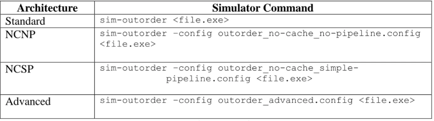
In this thesis, sim-outorder is used to generate the estimated WCET and BCET of a training program in various architectures (i.e. no cache no pipeline, no cache simple pipeline, advanced and standard). It has used four different settings to represent standard architecture (standard), no cache no pipeline architecture (NCNP), no cache simple pipeline architecture (NCSP) and advanced architecture (advanced) as configuration executable files. The <file.exe> given in every command is a file produced after compiling c file using sslittle-na-sstrix-gcc which is a SimpleScalar compiler.

Architecture Simulator Command

Standard sim-outorder <file.exe>

NCNP sim-outorder –config outorder_no-cache_no-pipeline.config <file.exe>

NCSP sim-outorder –config

outorder_no-cache_simple-pipeline.config <file.exe>

Advanced sim-outorder –config outorder_advanced.config <file.exe> Table 1: Hardware architecture vs. simulator command

2.2 SWEET

SWEET (SWEdish Execution Tool) shown in Figure 3, is a tool which is developed at Mälardalen University, C-Lab in Paderborn, and Uppsala University [1, 11].

Figure 3: Architecture of the SWEET timing-analysis tool [1]

SWEET is developed in a modular fashion in order to allow different analysis and tool parts to work quite independently. It is designed to conform to the scheme of WCET analysis consisting of flow analysis, a processor-behavior and an estimate calculation. SWEET has some functionality that offers as a timing analysis tool:

(16)

16

1. Automatic flow analysis at the intermediate code level 2. Integration of flow analysis and a research compiler

3. The connection between flow analysis and processor-behavior analysis 4. Instruction cache analysis for level-one caches

5. Pipeline analysis for medium-complexity RISC processors

6. A variety of methods to determine upper bounds based on the results of the flow and pipeline analysis

In SWEET, the flow analysis is integrated with a research compiler in previous version. But the current version of SWEET instead uses the ALF language for its analysis, rather than the internal format of the compiler. The use of ALF makes SWEET compiler-independent; if there is a translator into ALF, then SWEET can analyze the code. The flow analysis is performed on the intermediate code (IC) of the compiler, after the structural optimizations is done. To find timing effects across sequences of two or more blocks in a code consecutive simulation runs is done starting with the same basic block of the code. The analysis in SWEET assumes that there is a known upper bound on the length of the block sequences that can exhibit timing effects [1].

SWEET uses the language ALF as input for its flow analysis. ALF is a language mainly intended to be used in conjunction with WCET analysis [5]. ALF will be discussed in detail in the next section.

2.3 ALF (ARTIST2 Language for WCET Flow Analysis)

ALF is a language used for flow analysis for WCET calculation. It is an intermediate language which was mainly developed for flow analysis instead of code generation. It is also designed to represent a code on source-level, intermediate-level and binary-level through direct translation. It maintains the information in the original code while performing a precise flow analysis. ALF is a sequential imperative language which has a fully textual representation which makes it seems as an ordinary programming language though it is generated using a tool rather than written by hand [4].

2.3.1 Syntax

The syntax of ALF is similar to the LISP programming language which makes it easy to parse and read. ALF uses the same prefix notation as in LISP, but with curly brackets “{”, “}” as parentheses as in Erlang. An example is

{dec_unsigned 64 0}

which denotes the unsigned 64-bit constant 0 [4].

ALF is an imperative language with standard semantics based on state transitions. The state consists of the contents in data memory, a program counter (PC) holding the label of the current statement to be executed, and some representation of the stacked environments for function calls [4].

(17)

17 Example of ALF program

The following C code: if (x>y) z = 42;

Equivalently it can be translated into ALF as follows:

{ switch { s_le 32 { load 32 { addr 32 { fref 32 x } { dec_unsigned 32 0 } } }

{ load 32 { addr 32 { fref 32 y } { dec_unsigned 32 0 } } } } { target { dec_unsigned 1 1 }

{ label 32 { lref 32 exit } { dec_unsigned 32 0 } } } } { store { addr 32 { fref 32 z } { dec_unsigned 32 0 } } with { dec_signed 32 42 } }

{ label 32 { lref 32 exit } { dec_unsigned 32 0 } }

The if statement of the C program is translated to a switch statement, jumping to the exit label if the (negated) test becomes true (return one). The test uses the s_le operator (signed less-than or equal), taking 32 bit arguments and returning a single bit (unsigned, size one). Each variable is represented by size 32-bit frame.

ALF AST is an abstract Syntax tree, is a tree representation of the abstract syntactic structure of source code after translated to ALF statement, built by parsers and additional information is added to the AST by semantic analysis. The syntax is known as abstract as it does not give all details as in a real syntax.

2.3.2 ALF and SWEET

ALF is used as input to the WCET analysis tool SWEET. The figure shown below describes the uses of ALF in conjunction with SWEET.

Figure 4: The use of ALF with the SWEET tool [4]

First the input program code is read, which is represented in different formats and levels. Then the output is given in the generic ALF format. Then the ALF code is used as an input to the flow analysis in SWEET which outputs the results as flow constraints on the ALF code entities. Using the mapping information created earlier, these flow facts can be mapped back to the input formats [4].

(18)

18 2.3.3 C to ALF Conversion

SWEET cannot perform its analysis directly on C source or executable files. In order to achieve its analysis SWEET uses the ALF format. As ALF is the only input to SWEET, there are a number of translators to ALF being developed. All three types of sources (i.e. source code, intermediate code and binary code) are covered in those translators. The C to ALF translator which has been used in this thesis can be found on the MELMAC website [33]. MELMAC is a tool that translates C source code to the ALF format. A shell script1has been used in this thesis to make easy the conversion of C to ALF when it is run in a Linux environment (i.e. OPENSUSE). The shell script takes a C source file and generates the corresponding converted ALF file as output [4, 6].

2.4 WCET Benchmarks

In recent years a number of WCET analysis tools have emerged: both fully-fledged commercial tools, and research tools. In order to compare these tools the associated methods and algorithms, require common set of benchmarks. The crucial evaluation metric is accuracy of the WCET estimates but there are other evaluation metrics which are equally important such as performance (i.e. scalability of the approach) and general applicability (i.e. ability to handle all code constructs found in real-time). In order to enable comparative evaluation of different algorithms, methods, and tools, it is very important to have easily available, thoroughly tested, and well documented common sets of benchmarks [7].

2.4.1 Mälardalen WCET Benchmarks

The Mälardalen benchmarks are small (all except two are less than 900 LOC) and assembled with the same goal as mentioned above in mind. All these benchmarks are written in C and were collected in 2005 from several researchers within the WCET field. The benchmarks contain a broad set of program constructs to support testing and evaluation of WCET tools. The complete set of Mälardalen benchmarks can be found in Mälardalen WCET Benchmarks web page [8]. The main categories of benchmarks are well-structured code, unstructured code, Array and matrix calculations, Nested loops, input dependent loops, inner loops depending on outer loops, switch cases, nested if-statements and floating-point calculations, bit manipulation, recursive code and automatically generated code. Some Mälardalen benchmarks used in this thesis are given below in Table 2.

Program Description Comments

bs Binary search for the array of 15 integer elements. Completely structured

cover Program for testing many paths. A loop containing many switch cases.

edn Finite Impulse Response (FIR) filter calculations A lot of vector multiplications and array handling

fdct Fast Discrete Cosine Transform A lot of calculations based on integer array elements fibcall Iterative Fibonacci, used to calculate

fib(30)

Parameter-dependent function, single-nested loop

fir Finite impulse response filter (signal processing algorithms) over a 700 items long sample

Inner loop with varying number of iterations, loop-iteration

(19)

19

dependent decisions janne_complex Nested loop program The inner loops number of

iterations depends on the outer loops current iteration number ns Search in a multi-dimensional array Return from the middle of a

loop nest, deep loop nesting (4 levels)

nsichneu Simulate an extended Petri net Automatically generated code with more than 250 if-statements

Table 2: Some Mälardalen benchmark programs [7]

Single-path/multi-path benchmarks and inputs to the benchmarks: If a program runs the same path regardless of the inputs then it is a single-path program while multi-path program is a program where the execution path can differ for different inputs. But in reality most programs are run with different inputs in different invocations. During analysis of WCET, it is important to know the possible values of the input variables. In general, in order to obtain tight program flow constraints from the flow analysis, the input value needs to be constrained as much as possible. The possible input variables for an embedded program or task (possibly written in C) can be:

 Values read from the environment using primitives such as ports or memory mapped I/O,

 Parameters to main() or the particular function that invokes the task, and

 Data used for keeping the state of tasks between invocations or used for task communication, such as external variables, global variables or message queues.

In order to be able to test and evaluate such input dependency, multiple input values have been defined for some of the benchmarks. The inputs are provided as intervals i.e. limits to the inputs. The inputs are stored on the Mälardalen WCET Benchmarks web page [8] as “input annotations” (.ann files) in SWEET format [7].

2.5 Mathematical Equations

In this section the most important mathematical formulas, used to develop the timing model that will predict the BCET/WCET of a program, will be briefly discussed. Section 2.5.1 presents the linear equation followed by least-square methods in Section 2.5.2 and finally simulated annealing in Section 2.5.3 is discussed.

2.5.1 Linear Equation

A Linear equation is “an algebraic equation in which each term is either a constant or the

product of a constant and the first power of a single variable” [13]. It is an equation in the

form of

where is unknown [16]. The name “linear” comes from the set of solutions of such an equation which forms a straight line in the plane [13].

(20)

20

and can be also written as a weight for a column vector in a linear combination:

The vector equation is equivalent to a matrix equation of the form

where is an

x

matrix, is a column vector with entries, and is a column vector with entries [12].

2.5.2 Least-squares method

The Least-squares method is one of the standard mathematical approaches to approximate solution of sets of equations in which there are more equations than unknowns. It is the simplest and most commonly used form of linear regression. The most significant application is in data fitting where the best fit is found when the sum of squared residuals (i.e. the difference between an observed value and the fitted value provided by the model) is minimized [14, 17].

Figure 5: Data fitting using least-square [17]

The Least square method is categorized into linear and non-linear least squares, depending on whether or not the residuals are linear in all unknowns. There is a close-form solution which

(21)

21

can be evaluated in a finite number of standard operations for linear least-squares problem [14].

As mentioned above, the objective of the least-square method is to adjust the parameters of a model function to best fit a data set, or a technique applied in the form of linear regression through a set of points that provide a solution to the problem of finding the best fitting straight line, . A simple data set can have points of data pairs ,

where an independent variable, while is is a dependent variable whose value is found by observation. The fitting curve has a deviation (error) from each data point, i.e.,

, , …, . Then the best fitting curve has the property

that minimizes the sum of squares as shown:

Detailed information about least-squares method can be found in [14, 17, 18 and 21].

2.5.3 Simulated Annealing

Simulated annealing (SA) is a probabilistic technique which can find an optimal solution of a cost function that may possess several local minima [15]. In SA, when the physical process is emulated, the solid part gradually cools down and reaches “frozen” stage which happens at a minimum energy configuration.

Each iteration of SA algorithm randomly generates a new point. The distance between the new point and the current point is determined by the probability distribution with a scale proportional to the temperature. The SA algorithms collects all the new points that lower the objective including certain probability that raise the objective, but SA tries to avoid a local minima in early iteration by exploring a better solution globally [20].

The probability of taking a step is determined by the Boltzmann distribution as,

if , and when

Temperature T is inversely proportional to the energy difference . The temperature T is initially set to a high value and a random walk is carried out at that temperature. According to the cooling schedule, for example: where is slightly greater than 1 [25]. This method is an easy-to-implement, probabilistic approximation algorithm, (even though the structure of the problem might not be fully understood) which is able to produce good solutions for an optimization problem [19].

(22)

22

3. TIMING MODELS

In this section, the identification of linear timing model is done is going to be discussed in detail in order to grasp the idea behind the work of this thesis from the RNTS2011 paper [2]. Moreover, this thesis is the evaluation and extension of the result of this paper and some results of this thesis has been used in the RNTS2011 paper.

3.1 Identification of Linear Timing Models

The linear timing model identification is done assuming that the source language is emulated by an abstract machine which leads to tracing the virtual instruction in the source language of a program.

For each virtual instruction , the trace then contains occurrences of (the execution count of ). The linear timing model for the abstract machine computes the execution time

for a trace as

(1)

is a constant startup time, and , k =1,…,n are constant execution times for the respective virtual instructions. If we assume that is a virtual “startup” instruction, which occurs once in each trace, then (1) can be simplified as

(2)

The linear timing model for a code compiled with non-optimizing compilers executed on a simple hardware without features like pipelining or cache is expected to be more accurate than a code executed with more complex hardware architectures containing varying instruction execution times. Moreover, a code that has been heavily changed by using an optimizing compiler has a less accurate timing model. The goal is to find the best model which produces minimized deviation of predicted execution times from the real ones having the same number of observations. There is a measured execution time for each observation for the compiled binary and an array of execution counts for the emulated source code executed with the same inputs as the compiled binary. If we assume that we have made observations, the model predicts an array of execution times, where is an -matrix whose rows are the observed arrays of the execution count, and is an array of virtual instruction execution times. Let be the array of measured execution times for the different observations. The best model then amounts to finding a , that minimizes the overall deviation of from [2].

There are various ways to define the overall deviation and the Euclidean distance is used for this purpose:

(23)

23

The least-square method (LSQ) will find a that minimizes . The minimization of the overall deviation can also be heuristically done using SA which is applied in the

experiments.

3.2 Early Timing Analysis Approach

After training programs were designed, they were compiled and executed on target hardware or a simulator for it. As mentioned earlier, the SimpleScalar simulator is used in this thesis in order to ease the task. SimpleScalar was configured to simulate required architecture with a variety of different features, and it records the number of cycles needed to execute the program on the virtual hardware. The number of cycle values forms a vector [2].

Following that the training programs were translated to an intermediate format ALF language using the C-2-ALF translator as mentioned in Section 2.3.3, which provides the virtual instruction set. The execution counts for the ALF instructions were produced after SWEET interprets the ALF code which forms the matrix [2]. Then the model has been identified, i.e. the vector was determined using the LSQ method and SA (see Section 2.5). The last step is to use the model for timing analysis which could be done either through simulation or a static timing analysis. SWEET has been used to do both simulation and approximate static WCET analysis on source level using the timing models. ALF timing models are used to extend the interpretation mode of SWEET to provide timing estimates during simulation as shown in Figure 6.

Figure 6: Early-Timing analysis approach [2]

3.3 How are training programs constructed?

One important aspect of timing model identification is selecting good and an adequate number of training programs. The training programs used are synthetic program suites which allow more control over the virtual instruction traces by avoiding problems either with linear dependency or highly correlated execution counts. In this thesis, training program suites for three scenarios are designed; simple architecture, advanced architecture and floating-points.

(24)

24 3.3.1 Training programs for Simple Architecture

The training program suites for simple architecture are constructed as follows

 The first program is the “empty” program. Execution yields the startup time for a program (i.e. the time for a virtual RUN_PROG statement):

int main() {}

First this program is put in the suite, as every emulation of virtual instructions for a source program will execute RUN_PROG.

 Any nonempty C program must contain an assignment. Such a program must execute at least one virtual STORE instruction. Thus, the next program executes exactly one STORE:

int main() {int j=17;}

 Correspondingly, a third program executes along with STORE and RUN_PROG a LOAD instruction. Until the full set of instructions is executed the program suite continues with a series of simple programs executing each remaining instruction. For example, INT_MULT instruction:

int main() {int j=42; j=j*3}

The number of function calls was equal to the number of executed RETURN instructions. In order to avoid this dependency, which can occur due to RETURN instruction, it is replaced by a superinstruction carrying their added execution times which will help to yield a lower-triangular execution count matrix with nonzero diagonal entries. There were no linear dependencies between the column vectors of such matrices. As there was exactly one program execution per instruction, becomes a quadratic matrix. Furthermore, the absence of linear dependency causes to be invertible and the linear system can be solved directly to yield such that .

3.3.2 Training programs for Advanced Architecture

The advanced architecture, having caches and pipeline features, will cause instructions to have highly context-dependent execution times. In order to have the model capturing the influence of the context on the execution time, the “real” instructions must be executed in a variety of contexts when identifying the timing model. Moreover, in order to capture the cache and pipelining influence, longer instruction sequences must be executed. One way of accomplishing this is to introduce loops in the code. The advanced architecture test suite is built up on simple architectures and extends the programs with loops executing the instruction under test a number of times. This extension gives reasonably good results even though it does not capture more complex timing effects involving several different instructions [2].

Some instructions were invariably needed during the loop introduction in the code; a

(25)

25

the loop counter, some test instruction to decide the exit condition, and a JUMP to return to the entry point of the loop. This resulted in a matrix without lower triangular execution count. But the execution counts made linearly independent by introducing several loops executing different arithmetic operations to increment/decrement the loop counter, and different test instructions to break the loop. In order to break the possible linear dependencies to instructions (like JUMP) that appear in all loops, a third part of the code executes the loop body outside any loop. The linear dependencies between any instructions has been broken and also the correlation minimized if the training program has been executed a number of times, with different loop bounds set in a linearly independent fashion.

An example of a training program for INT_MULT, consisting of two independent loops and a section with straight-line code:

int main () {

int max1 = …; int max2 = …; int i,j;

for (i=1; i<=max1; i++) { j = I; j = j*3;

}

for (i=max2; i>0; i--) J = I; j = j*3; }

J = i; j = j *3; }

INT_MULT would always been executed as many times as the ADD that increments i, and the test operation that compares i with max1 if only the first loop was present. As a result, linear dependency would have been created between these execution counts. A different test operation is created using a second loop which uses SUB to decrement the loop counter.

Using max1 and max2 a number of executions could be made in such a way that the resulting execution counts for the involved virtual instructions are linearly independent. But both loops had a single JUMP each and INT_MULT will still be the same no matter what max1 and max2 are and in order to break linear dependency, the third appearance of the loop body has been added. This is automated to generate training programs automatically and the constant max1 and max2 can be varied [2].

3.4 Model Identification

There have been different approaches tried to the problem of choosing such that predicts the execution time well for the compiled binary, running on the chosen target platform. Even though LSQ (see Section 3.1) gave best fit for the set of programs by selecting real-valued weights to minimize distance, it can yield models that did not predict the execution time well for programs outside the training set. For example, it could yield negative cycle counts for instructions which are unrealistic. Moreover, it may yield very poor predictions for programs that execute instructions frequently as compared to other

(26)

26 instructions.

They have used also a more general search method that allows more freedom in specifying constraints and objective function. The SA approach has been used, in which each step of the SA algorithm replaces the current solution by a random solution from the neighborhood. If the result of SA is better, it is accepted or else it may still be accepted with a probability that depends both on the difference between the subsequent objective function values, and on a global parameter (the “temperature”). As the temperature is decreased during the process, jumps leaving the local solution space will become less and less likely, so eventually the result will stabilize.

Adapting SA to minimize is easy, and it is done according to the following:  All elements in are initialized to zero

 For producing a solution in the neighborhood of , its elements will be randomly incremented or decremented by one, or kept as is (while upholding any imposed constraints on the solution).

SA has been executed several times with varying parameters to get the best result since SA is very sensitive to its steering parameters like temperature.

3.5 Experiment done by Mälardalen WCET group

The MDH WCET group has already made an evaluation on the precision of the identified models, as well as the influence of the training program suite. They have used two sets of training programs for advanced architecture and simple architecture and they have tried both LS and SA as shown in Table 4. Using a distinct set of programs consisting of fifteen programs from the Mälardalen WCET Benchmark Suite, the models were evaluated as shown in Table 3. Table 3 gives some basic data about the programs, including lines of C code (#LC), the number of functions (#F), loops (#L), and conditional statements (#C).

Program #LC #F #L #C bs 114 2 1 3 cover 640 4 3 6 edn 285 9 12 12 Esab_mod 3064 11 1 292 fdct 239 2 2 2 fibcall 72 2 1 2 fir 276 2 2 4 inssort10 92 1 2 2 inssort15 92 1 2 2 inssort20 92 1 2 2 inssort30 92 1 2 2 jcomplex 64 2 2 4 loop3 76 1 150 150 ns 535 2 4 5 nsichneu 4253 1 1 253

Table 3: Benchmark Programs [2]

First a comparison was done between predicted and real running time result generated by running each benchmark with its specified input (all these benchmarks have their

(27)

hard-27

coded inputs). From the results, estimations are taken how well the derived timing models predict real running times. Then, by removing the hard-coded inputs for some selected benchmarks, they changed the hard-coded inputs into programs having different paths through the code for different inputs. Later possible input values were defined for each selected benchmark. Finally, a static BCET/WCET analysis for these benchmarks was performed, so as to evaluate the precision of static timing analysis based on the timing models. The real best/worst case obtained using an exhaustive search over the possible inputs and compared with the static BCET/WCET estimates [2].

SWEET has been used for both single runs and the static analysis and it has a “single-path

mode” that can be used to emulate ALF code. SWEET is turned into a source-level

simulator estimating execution times using ALF timing models in extension of the single-path mode. Moreover, SWEET’s static analysis has been extended so as to perform BCET analysis on top of WCET analysis [2].

Both the training programs and benchmarks have been compiled using sslittle-na-sstrix-gcc with no optimization and for sim-outorder executes with its standard configuration in SimpleScalar. Sim-outorder simulates a processor with out-of-order issues of instructions, main memory latency 10 cycles for the first access and 2 cycles for the next accesses, memory access bus width 64 bytes, 1KB L1 instruction cache (1 cycle, LRU), no data cache, no L2 cache, no TLB’s, 1 integer ALU, 1 floating point ALU, and fetch width 4 instructions. The branch prediction is 2-level with 1 entry in the L1-table, 4 entries in the L2-table and history of size of 2.

The experiment done in [2] had selected benchmark programs that did not use floating-point instructions which make ALF use 31 different ALF instructions that has formed the virtual instruction set for the experiment. These instructions included program flow control instructions, LOAD/STORE, and arithmetic/logical instructions excluding floating-point arithmetic.

3.5.1 Training Programs

The “simple” training program suite has been used from Section 3.3.1. The average deviation obtained for the set of benchmark programs in Table 4 is 29%. This result showed that this suite is not well suited to identify models for architecture like sim-outorder.

In order to see the influence on precision of the predicted execution, the “advanced

architecture” suite tried by executing loops with varying number of iterations. As it has

been noted, architectural features like cache and branch predictors tend to yield shorter instruction execution times within loops which seemingly influence the identified model and its resulting precision. To estimate the influence a program suite instantiation “small” (loop iterating 7-17 times), “medium” extending “small” with instances of the programs iterating up to 29 times, and “big” extending “medium” with instances iterating up to 61 times is used. Furthermore, to see the influence on the precision they tried adding the “simple” training program suite. As a result a total of six test cases with different variations of the training program suite produced [2].

3.5.2 Model Identification Method

The LSQ and SA have been tried with different variations. For LSQ, both direct solution and with instruction execution times rounded to the closest integer, has been tried. The

(28)

28

outcomes showed that in both cases, there was no restriction on the instruction execution times: therefore, e.g., negative execution times were possible and would indeed appear sometimes.

The Euclidean deviation is used as an objective function for SA with three variations. In the first variation, SA was run without any constraints on the final solution and in the second run, with constraints that all virtual instruction execution times enforced to be non-negative. This was done to observe whether it would yield a better prediction when the constraints were added. In the third variation, the search space size was restricted for SA by enforcing an upper limit on virtual instruction execution times. This was created to shorten search times for SA; it was interesting and important to see whether the identified model precision was affected by it.

All these variations of LSQ and SA were tested with all six different training program suite combinations as shown in Table 4. The result shows the relative average deviation of predicted running times from measured running times.

Training suite LSQ LSQ rounded SA SA≥0 0≤SA ≤2× small 39% 34% 10% 10% 10% medium 50% 45% 14% 12% 12% big 64% 63% 16% 13% 13% small + simple 18% 17% 15% 10% 20% medium + simple 19% 15% 16% 10% 10% Big + simple 17% 14% 16% 10% 10%

LSQ: standard least squares method, LSQ rounded: LSQ rounded to closest integer SA: Simulated Annealing with no constraints on the solution

SA≥0: SA restricted to nonnegative instruction times, 0≤SA≤2×: SA additionally restricted from above

Table 4: Average deviation of predicted vs. real execution times for benchmarks with different model identification methods [2]

As shown in the above table, SA has much better result for all examples compared to LSQ but LSQ gave improved results when a simple training suite was added. Even rounding the LSQ result did not bring a significant change, whereas SA consistently gave the best results when restricted to nonnegative values. The restriction has a significant effect for the small + simple training suite which resulted in faster convergence in SA solutions in all cases.

The result obtained in [2] shows deviation between the measured and the predicted running time for the individual benchmark programs as shown in Table 5. All the programs have a deviation from close to zero up to about 20% except for cover which has an extreme outlier with more than 50% underestimation.

A subset of benchmark codes has been used to evaluate the approximate source-level timing analysis. Since the programs are multipath, in which execution times vary with inputs and their worst- and best-case input are known. Therefore, by running SimpleScalar with proper input, the real BCET and WCET could be approximated.

The result of the analysis is shown in Table 6 of [2], along with BCET and WCET recorded for SimpleSacalar. The result obtained is reasonable BCET and WCET estimate

(29)

29

as compared to the precision measured by the single execution times.

In [2], the model identification method was tried for advanced architecture, in which sim-outorder is configured to simulate a processor with some characteristics like out-of-order issues instruction, main memory latency 18 cycles for first access and 2 cycles for next accesses, 8KB L1 data and instruction caches, respectively (1 cycle), 256KB L2 data and instruction cache (6 cycles), all caches LRU, no TLB, 2 integer ALU's, 2 floating-point ALU's, fetch decode, issue, and commit width all 4 instructions, perfect branch prediction. Then the model identification was rerun for this hardware configuration and the best model obtained was by SA>=0 and evaluated the precision of the timing model using a single benchmark program run. The deviation obtained was 0-30% and the average deviation is 15%.

Program Model Measured Diff Rel. diff

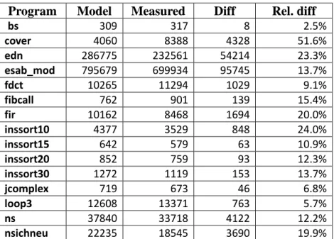
bs 274 317 43 13.6% cover 3515 8388 4873 58.1% edn 244189 232561 11628 5.0% esab_mod 698848 699934 1086 0.2% fdct 9250 11294 2044 18.1% fibcall 788 901 113 12.5% fir 6973 8468 1495 17.7% inssort10 3674 3529 145 4.1% inssort15 549 579 30 5.2% inssort20 729 759 30 4.0% inssort30 1089 1119 30 2.7% jcomplex 671 673 2 0.3% loop3 11999 13371 1372 10.3% ns 31897 33718 1821 5.4% nsichneu 19744 18545 1199 6.5%

Table 5: Predicted vs. measured times for single benchmark program runs [2] Program Model Measured Diff Rel. diff

bs 130 184 54 29.3% cover 1837 3605 1768 49.0% edn 140136 119291 20845 17.5% esab_mod 368743 408076 39333 9.6% fdct 4998 3940 1058 26.9% fibcall 283 377 94 24.9% fir 3923 4035 112 2.8% inssort10 2094 1678 416 24.8% inssort15 284 303 19 6.3% inssort20 379 395 16 4.0% inssort30 569 568 1 0.2% jcomplex 282 307 25 8.1% loop3 5017 6290 1273 20.2% ns 18758 18725 33 0.2% nsichneu 10969 10129 840 8.3%

(30)

30

4. PROBLEM DESCRIPTION, PROJECT SETUP and METHODS

The objective of this thesis is to evaluate the method used to build timing models, by evaluating the accuracy of the resulting timing models for a number of combinations of hardware architecture. The models have been built using predefined suites of test programs, using both the LSQ method and some variations of SA. To ease the task of measuring execution times, the hardware simulator SimpleScalar has been used as target hardware rather than real hardware. The thesis project started with analyzing the result that has been produced and published by the WCET group in RTNS11 paper [2].

The main hardware used in this thesis was a PC with Opensuse 11.4 version. To ease the task of measuring execution times is carried out by using SimpleScalar version 3.0e simulator. SimpleScalar can be configured to simulate a variety of processor architectures, and there exist a version of gcc that compiles C code to the SimpleScalar instruction set. This version of gcc allows using a number of different optimization levels. There have been four different configurations of SimpleScalar that simulated the NCNP architecture, NCSP architecture, Standard architecture and advanced architecture mentioned in Table 1. Moreover, alongside with SimpleScalar, SWEET has been used as one of the main software or tools in this thesis. So far, no version has been set on SWEET because it is a research prototype. SWEET was modified several times throughout the thesis by fixing bugs found in it. Some shell scripts has been used during the project setup and analysis because SWEET is a command based tool without any GUI. Firstly, the platform was set up after installing SimpleScalar and tried out with some Mälardalen benchmarks that have been used in Table 5. The next step was to install SWEET and attempt to execute some Mälardalen benchmarks in order to make sure that SWEET was installed properly. In both these startups of the project, only single-path mode was taken into account.

4.1 Virtual Instructions

The first step to identify a source-level timing model for a given combination of hardware configuration is to select a set of virtual instructions (such as arithmetic/logic operations, branching, function calls/returns etc). An abstract machine that can execute source code has been defined using the set of virtual instructions.

4.2 Analysis timing models using SimpleScalar

The following steps were involved for analyzing timing models with SimpleScalar.

i) The training program generator was an executable file and it has been executed to generate specific c-file training programs. The training program generator should be set according to the matter at hand to produce the specific training suite (for example, if floating-point benchmarks were used, we have to use the proper combination in order to identify the corresponding model).

ii) Then the training programs c files are compiled using this command: sslittle-na-sstrix-gcc $file.c –o $file.exe

in which $file is replaced with respective c file and outputs an $file.exe file. iii) Then it is executed using sim-outorder with different combinations of

(31)

31

SimpleScalar processor configurations and it produced the cycle counts for each exe file:

sim-outorder –config outorder_<processor configuration>.config $file.exe

where <processor configuration> is replaced by a specific SimpleScalar processor configuration of the hardware architecture and produces cycle counts for each training program suite.

4.3 Analysis timing models using SWEET

The following steps were involved for analyzing timing models with SWEET.

i) For SWEET, the first step was done to transform all the training program suite c-files to an intermediate format, ALF, which provides virtual instruction using a shell script. The c_to_alf_using_christers_machine.sh was a shell script that would run the C-2-ALF translator melmac on a machine where it was installed during the thesis project and written as follows:

c_to_alf_using_christers_machine.sh $file.c where $file.c is replaced with training program suite c-file

ii) Then the ALF file is executed to produce the count of statements occurrences (statements are like store, call… etc.)

sweet –i=file.alf –ae pu tc=st

where –i option represent input-files, which file.alf are the particular ALF files and –ae is used to give abstract execution to produce flow facts. The option pu is used when –ae should be run on code containing imports (i.e. undefined).

Both steps done in 4.1 and 4.2 are written together in a shell script2. The shell script is executed as follows:-

./produce-input-data.sh

which gives a matrix to produce a result line for an equation file in the form of , where is the result generated in 4.3 using SWEET and is generated in 4.2 using SimpleScalar. These results are written to Axb.csv file as an output of the shell script2.

4.4 Identification of Linear model

The output produced in Section 5.3, named Axb.csv, is fed to the file which is an equation solver, as input, in order to identify a linear timing model with an execution time for each virtual instruction from the measured execution times and recorded instruction counts.

./EquationSolver.sh –i58 Axb.csv

(32)

32

As mentioned in Section 3.4, the model identification is summarized into a shell script3 which takes Axb.csv and solves equations of the form A*x=b using three different algorithms, namely LU decomposition, linear regression and SA. The –i58 option is used to remove column 58 in Axb.csv which is a “RETURN” statement in order to avoid dependency as explained in Section 3.3.1. This will also create several CSV files in which all output files are summarized in overview.csv where the best vector is to the left of a corresponding CSV file with the same name as a headline of the left-most column in the directory [26].

4.5 Source Level Timing Analysis

A source level timing analysis is done based on the best vector produced in Section 4.4 using SWEET.

4.5.1 Single path timing estimates

i) An alf file is executed using SWEET

sweet -i=$file.alf -ae pu css vola=i tc=st,op

where –i

,

-ae and pu options has already been explained in Section 4.3. The css option is used to check if a single state is generated, i.e., it throws run-time error if more than one state is generated during the abstraction execution. $file.alf is replaced by a particular Mälardalen WCET benchmark. Moreover, tc=st,op is a type counting which counts the number of occurrences for each type during an execution. In this particular situation, it counts the occurrence of statements (i.e. store, call... etc) and operators. This produces predicted times for single benchmark programs, similar to Table 5 and 6.

ii) The same procedures as Section 4.2 is done using SimpleScalar except that $file is replaced by a benchmark file and produces measured times for single benchmark programs.

Both i) and ii) are summarized in a shell script4. The shell script is executed as follows: - ./produce-output-data.sh <bestvector.csv> <benchmarks>

where bestvector.csv is produced in Section 4.4. <benchmarks> is replaced by a directory containing all benchmarks selected to be used for single path estimates. A for-loop is iterated throughout the whole benchmarks. The output of this shell script is written to compare.csv file containing measured and predicted timing estimates into two different columns.

4.5.2 Multi-path timing estimates

The source level timing analysis is also evaluated using a subset of benchmark codes which are multipath programs. The BCET and WCET can been known for such programs since BCET and WCET of the inputs are known. This thesis has only worked to estimate BCET and WCET of proper benchmarks using SWEET. The measured BCET/WCET using SimpleScalar is not included since it is not a priority in this thesis.

During this thesis, some benchmarks, which has been evaluated using multi-path source level

3

EquationSolver.sh