Weather data for building simulation
New actual weather files for North Europe combining
observed weather and modeled solar radiation
Lukas Lundström
School of Sustainable Development of Society and Technology Subject: Building Technology
Advanced level 15 credits
Master program in Energy Optimization for Buildings BTA305
Supervisor: Robert Öman Examiner: Adel Karim
Västerås, Sweden, 2012-12-07
DEGREE PROJECT, 15 ECTS
School of Sustainable Development
of Society and Technology, HST
2
Summary
Dynamic building simulation is increasingly necessary for accurately quantifying potential energy savings measures in retrofit projects, to compliant with new stricter directives from EU implanted into member states legislations and building codes. For good result the simulation model need to be accurately calibrated. This requires actual weather data, representative for the climate surrounding the given building, in order to calibrate against actual energy bills of the same period of time. The main objective of this degree project is to combine observed weather (temperature, humidity, wind etc.) data with modeled solar radiation data, utilizing the SMHI STRÅNG model system; and transform these data into AMY (Actual Meteorological Year) files to be used with building simulation software. This procedure gives actual weather datasets that will cover most of the urban and semi urban area in Northern Europe while still keeping the accuracy of observed weather data. A tool called Real-Time Weather Converter was developed to handle data retrieval & merging, filling of missing data points and to create the final AMY-file.
Modeled solar radiation data from STRÅNG had only been validated against a Swedish solar radiation network; validation was now made by the author with wider geographic coverage. Validation results show that STRÅNG model system performs well for Sweden but less so outside of Sweden. There exist some areas outside of Sweden (mainly Central Europe) with reasonable good result for some periods but the result is not as consistent in the long run as for Sweden.
The missing data fill scheme developed for the Real-Time Weather Converter does perform better than interpolation for data gaps (outdoor temperature) of about 9 to 48 hours. For gaps between 2 and 5 days the fill scheme will still give slightly better result than linear interpolation. Akima Spline interpolation performs better than linear interpolation for data gaps (outdoor temperature) in the interval 2 to about 8 hours.
Temperature uncertainty was studied using data from the period 1981-2010 for selected sites. The result expressed as SD (Standard Deviation) for the uncertainty in yearly mean temperature is about 1˚C for the Nordic countries. On a monthly basis the variation in mean temperature is much stronger (for Nordic countries it ranges from 3.5 to 4.7 ˚C for winter months), while summer months have less variation (with SD in the range of 1.3 to 1.9 ˚C). The same pattern is visible in sites at more southern latitudes but with much lower variation, and still lower for sites near coast areas. E.g. the cost-near Camborne, UK, has a SD of 0.7 to 1.7 ˚C on monthly basis and yearly SD of 0.5 ˚C.
Mean direct irradiance SD for studied sites ranges from 5 to 19 W/m2 on yearly basis, while on monthly basis the SD ranges from 40 to 60 W/m2 for summer months. However, the sample base was small and of inconsistent time periods and the numbers can only be seen as indicative.
The commonly used IWEC (International Weather for Energy Calculations) files direct radiation parameter was found to have a very strong negative bias of about 20 to 40 % for Northern Europe. These files should be used with care, especially if solar radiation has a significant impact of on the building being modeled. Note that there exist also a newer set of files called IWEC2 that can be purchased from ASHRAE, these files seems not to be systematically biased for North Europe but haven’t been studied in this paper.
3
The STRÅNG model system does catch the trend, also outside of Sweden, and is thus a very useful source of solar radiation data for model calibration.
Keywords: Energy, Building, Simulation, Model, Weather, Data, Actual, Historic, AMY, STRÅNG, Solar, Radiation, Missing data, Data gaps, Fill scheme, Interpolation, Akima
4
Table of content
Summary ... 2
Table of content ... 4
Terms and abbreviations ... 6
Introduction ... 8 1 Objectives ... 8 1.1 Limitations ... 9 1.2 Methods ... 9 1.3 1.3.1 Formulas used to estimate prediction power ... 10
Background ... 12
2 Weather data and energy balance calculation ... 12
2.1 2.1.1 Hourly weather data files ... 13
Solar radiation data by STRÅNG ... 14
3 Validation ... 14
3.1 3.1.1 Geospatial validation ... 15
3.1.2 Temporal validation ... 16
3.1.3 Correlation: direct, global and diffuse ... 17
“Real-Time Weather Converter”-software ... 19
4 Data retrieval ... 19 4.1 Data conversion ... 20 4.2 4.2.1 Interpolation ... 21
4.2.2 Longer data gaps ... 21
4.2.3 Testing interpolation and fill schemes ... 22
4.2.4 Time shift ... 23
4.2.5 Diffuse radiation ... 24
4.2.6 EnergyPlus and IDA ICE weather files ... 24
Weather data impact and uncertainty ... 26
5 Temperature ... 26
5.1 Solar radiation ... 27
5.2 Testing on an IDA ICE model ... 31
5.3 ASHRAE IWEC weather files ... 33
6 Conclusions ... 35 7 Discussion ... 36 8 References ... 38
5
Appendix A C# sample codes ... 40
Appendix A.1 C# method for filling missing data gaps ... 40
Appendix A.2 Part of the method used to load STRÅNG-data from file ... 41
Appendix B Tables ... 42
Appendix B.1 Geospatial validation results ... 42
Appendix B.2 Descriptive statistics: mean monthly temperatures [˚C] ... 44
6
Terms and abbreviations
Global radiation The total of direct and diffuse solar radiation received by a unit horizontal surface. Also known as total radiation
Direct radiation Solar radiation received directly from the solar disk on a surface perpendicular to the sun's rays, also known as beam radiation
Diffuse radiation Solar radiation energy falling on a horizontal surface from all parts of the sky apart from direct radiation. Also known as sky radiation.
Irradiance Incident radiation energy per unit time and area [W/m2] Irradiation Time integrated irradiance [Wh/m2]
AMY Actual Meteorological Year. Actual (historic) weather data for a specific location and specific year.
TMY Typical Meteorological Year. Weather data for a specific location artificially generated from a much longer period of time than a year. Selected so that it presents the range of weather phenomena, while still giving annual averages that are consistent with the long-term averages.
SMHI Swedish Meteorological and Hydrological Institute
IWEC International Weather for Energy Calculations weather data files, available for free. Refers to the IWEC files created in 2000
IWEC2 A new set of International Weather for Energy Calculations weather data files that can be purchased from ASHRAE
STRÅNG Model system by SMHI that produces instantaneous fields of solar radiation related parameters
ISD Integrated Surface Database consists of global hourly and synoptic observations compiled from numerous sources into a single database.
WRDC The World Radiation Data Centre
BSRN Baseline Surface Radiation Network
eKlima Web portal which gives free access to the climate database of the Norwegian Meteorological Institute
MBD Mean Bias Difference
RMSD Root Mean Square Difference
7
SD Standard Deviation
BIM Building Information Modeling is a digital representation of physical and functional characteristics of a facility
8
Introduction
1
The buildings sector accounts for approximately 40 % of the total energy consumption in the European Union (EU). Therefore, reduction of energy consumption and the use of energy from renewable sources in the buildings sector are central measures needed to reduce the EU energy dependency and greenhouse gas emissions. Increased energy efficiency in the EU is emphasized in order to achieve a 20 % reduction in the EU energy consumption by 2020. In 2010 the EU adopted the Energy Performance of Buildings Directive (EPBD) 2010/31/EU which is the main legislative instrument that aims to reduce the energy consumption of buildings. In Sweden it is implemented in the Swedish building code BBR where BBR 19 was adopted on 1 of January 2012.
In connection with the energy requirement in the Swedish building code a general advice was issued (Swedish Building Regulation BFS 2011:26) that an energy balance calculation shall be made during the design of a building, as to verify that the proposed building will meet the requirements. Any uncertainty in the calculations should be handled by an appropriate safety margin applied so that there is no risk that the energy requirements are exceeded. With reduced energy consumption due to stricter legislation and regulation the necessary safety margin increases relatively. This in turn leads to a need for more accurate energy balance calculations.
Building simulation software are tools that can be used to achieve the higher accuracy demand. To get good results these software requires accurate weather data. Actual Meteorological Year (AMY) files are needed for calibration of the building model. This weather data need to accurately represent the climate surrounding the building during the time that data was collected.
This degree project studies how to obtain AMY-files by combining observed weather data from the Integrated Surface Database (ISD) with modeled solar radiation data from the modeling system called STRÅNG developed and run by SMHI (Swedish Meteorological and Hydrological Institute). The degree project is made as a proof of concept: where a tool called Real-Time Weather Converter was developed, consisting of following features:
Retrieving data from ISD and STRÅNG databases Data extraction and merging of data
Data editing in tabular form
Interpolation and a fill scheme for missing data
Creation of AMY-files, supporting IDA ICE and EnergyPlus weather file formats
Generally temperature is the weather parameter with strongest impact on building simulation while solar radiation has less impact. Observed temperature data exists for most urban locations while ground observation of solar radiation, particularly direct radiation, is sparse. Using ISD for
temperature data and STRÅNG data for solar radiation gives weather files that will cover most of the urban and semi urban area in Northern Europe while still keeping the accuracy of observed
temperature data compared to using interpolated values.
Objectives
1.1
The main objective is to combine observed weather (temperature, humidity, wind etc.) data with modeled solar radiation data (from SMHI STRÅNG model system
)
, and to create AMY-files to be used with building simulation software. To achieve this, following interim targets are set up:9
Develop a prototype of a tool able to produce AMY-files from observed weather data and modeled solar radiation from STRÅNG.
Test the tool.
Validate solar radiation data from STRÅNG modeling system for the whole covered geographic area.
Study uncertainty and impact of weather data parameters on dynamic building energy simulation.
Limitations
1.2
This paper study hourly weather data that are required by dynamic building simulation software, with focus laid on AMY-files. Other methods for calculating weather data impact on an energy balance are not considered.
Validation is done on global radiation data from STRÅNG, direct radiation is not validated as there are too few sources available of observed direct radiation. Validation is done on daily data because of the “time shift” problem (Chapter 4.2.4) in the hourly data and because there are more sources of observed daily data available than for hourly data. It is expected that the quality of the daily data also reflects the quality of hourly data. There are many sources for error in the validation procedure:
Measured solar radiation data used for the validation origin from different sources, there can be difference in how measurements are performed and how the data are processed.
The measured value is taken as the actual value, but the difference between a measured and an actual value can in reality be significant. A radiation measurement can be erroneous e.g. because of incorrect sensor leveling, complete or partial shading, electric field near cables, station shut-down as well other uncertainty sources like dust, snow, dew and bird droppings. The modeled values represent an average value of grid area (about 120 km2), while ground
observations are point values.
Other weather parameters from ISD are assumed to be of good quality and are not tested in any way.
The Real-Time Weather Converter tool is developed as a prototype, meaning that many methods can/need to be further developed.
Methods
1.3
First the tool Real-Time Weather Converter was developed in the Visual Studio 2010 environment using C# code. This tool was later used to acquire data from STRÅNG and ISD. A “fill algorithm” for longer data gaps was developed and tested together with three interpolation schemes to determine which method was best suited for different length of data gaps (Chapter 4.2.3).
For the validation of STRÅNG (Chapter 3.1) global radiation was chosen as there was most data available for this solar radiation component. But building simulation software use the direct and diffuse solar components, therefore the relationship between the different solar radiation
components were determined by a correlation study (Chapter 3.1.3). Building simulation software usually use hourly weather data. But daily mean values were used for the validation because of the “time shift” problem (Chapter 4.2.4) in the hourly data and because there are more sources of observed daily data available than for hourly data. The year 2007 was chosen for the geospatial
10
validation as it was the year where there was most data available from all sources. Observed solar radiation data was gathered from four sources:
Most of the global daily radiation origin from the World Radiation Data Centre (WRDC, u.d.) using the html web archive for 2007 and earlier and the Java applet for data after 2007 . The data is given as daily irradiation [J/cm2] and was transformed to daily irradiance [W/m2] by ( ) ( ) ( ) ( ). Quality flags were not considered, meaning that also data of uncertain quality were included.
For Norway the eKlima (Norwegian Meteorological Institute, u.d.) web portal was used. The data is given in hourly irradiation [Wh/m2]. Transformation to daily irradiance was done by summing up all positive values per day and dividing with 24 [h]. Quality flags were not considered.
For direct radiation component the Baseline Surface Radiation Network (BSRN, u.d.) was used. Data was retrieved using the PANGAEA (PANGAEA, u.d.) Open Access library’s Data Warehouse service, where data can be retrieved in minutely, hourly, daily, monthly or yearly mean values [W/m2].
SMHI provided hourly solar radiation data for Norrköping for the period 2006 to 2007. Daily and monthly STRÅNG data are arithmetic mean of hourly data acquired by using the Real-Time Weather Converter tool. The validation calculation was done using formulas described in Chapter 1.3.1, within a Visual Studio C# Excel Workbook, which allowed automation of the otherwise quite tedious procedure. Only data points where data existed for both observed and modeled data were included.
As to establish the degree of significance of accurate actual solar radiation and temperature in a building simulation calibration an uncertainty study was undertaken (Chapter 5), the IBM SPSS Statistics software was used do acquire the descriptive statistics. Also a study of impact was started but the real energy consumption data for the used IDA ICE model (Chapter 5.3) was too unreliable to draw any general conclusion and should more be seen as a test.
In the progress of the work it was recognized that the ASHRAE IWEC files have strong negative bias, to determine to what degree a short study was undertaken (Chapter 6).
1.3.1 Formulas used to estimate prediction power
Mean Bias Difference (MBD), more commonly known as Mean Bias Error (MBE). The word difference is used instead for error as the measured (observed) value is not necessary a perfect reference.
∑( )
(1)
Mean Absolute Difference (MAD),
∑| |
11
Root Mean Square Difference (RMSD) is used to measure accuracy of the model. The difference (error) occurs because of randomness or because the model doesn't account for information that could produce a more accurate estimate. Since the difference ( ) is squared, large errors will have a stronger impact.
[ ∑( )
]
⁄
(3)
Relative MBD, MAD and RMSD are defined as normalized to the mean of the measured values.
̅ [ ∑( )
] [ ∑
] (4)
Calculated (modeled) value Measured (observed) value Number of counts
12
Background
2
Calculations of the energy balance of buildings require a lot of input data that can be classified in three groups1:
Technology. Building technology with thermal insulation, air tightness, heat capacity, size & shape of the building etc. Heating and ventilations technology with air flows, heat recovery, heat pump, time control, demand control, utilization of solar energy, waste heat, natural heat etc. Efficiency regarding the use of electricity for different purposes in the building. Human behavior. Has a very strong influence in many ways with different use of hot water
and electricity, different settings for the indoor temperature, different maintenance etc. Weather data. Outdoor temperature, solar radiation, humidity, wind etc.
When calculating the energy balance there are a lot of uncertainties regarding input data within all these three groups. This means that the difference can be significant when comparing the results from calculations with the actual energy use from measurements (readings) of electricity and for example district heating. All the three groups of input data are important for differences between calculated and actual energy use.
Weather data and energy balance calculation
2.1
There exist several methods to calculate an energy balance for a building that don’t require hourly weather data. Two methods commonly used in Sweden, heating degree day and a method
developed at KTH (Royal Institute of Technology), are shortly described below:
Heating degree days are defined relative to a base (also called limit) temperature (17˚C is commonly used the Nordics). This value refers to an imagined “limit” between active and passive heating where active heating is assumed to reach 17 °C indoor temperature while passive heat on average adds 3 °C so that 20 °C is achieved indoors. To account for the fact that solar radiation reduces the degree days a threshold value for the outdoor temperature can be used, this value represents the temperature above which no heating is needed. In Sweden following threshold values are commonly used: April +12° C, May – July +10° C, August +11° C, September +12° C and October +13° C (SMHI, 2011). The monthly heating degree days is calculated as the sum of the difference of the daily mean
temperature and the base value (17˚C), but just for days for which the mean temperatures reaches below the threshold values.
A method developed at KTH to calculate solar radiation gain through windows by categorizing days into three groups: clear, semi-clear and overcast days. Tables, based on 30 years of data, give the amount of each type of day for every month. Expected solar radiation values for the three day types are given in tables with a resolution of 2 latitude degrees, and for different angles and orientations. These values are then multiplied with the amount of day type in question, which result in an estimate of the solar radiation gain through windows in kWh/m2. (Höglund, et al., 1985). The same approach is utilized in the Consolis Energy+ excel tool developed by Gudni Jóhannesson in 2005.
These two methods are fairly straight forward to use and give reasonable good result. But with demand for reduced energy consumption in buildings, advances in computer technology and the
13
implementation of BIM the building industry is moving towards using building simulation software for energy calculation more and more.
2.1.1 Hourly weather data files
Dynamic building simulation software (e.g. IDA ICE and EnergyPlus) uses weather files consisting of parameter describing the weather, with a temporal resolution of at least one hour. Such a file would then consist of 8760 rows for every hour of the year, and a number of columns with parameters describing the weather. An IDA ICE weather file consist of following parameters: time, outdoor air temperature, humidity, wind direction, wind speed, direct radiation and diffuse radiation. An EnergyPlus weather file consists of 35 parameters, but not all are actually used and the parameters above are enough for creating a usable weather file.
In the Nordics temperature is regarded as the weather parameter with strongest influence on an energy balance followed by solar radiation (Jylhä & et.al., 2011). Humidity has impact mainly if the outdoor air needs to be cooled under the dew point temperature, which seldom is the case in north Europe. Local wind speed and wind direction around a building can be different from that of the nearest observation station, but their influence on whole are considered relatively low2.
Whether data files can be classified in three main classes:
Typical Meteorological Year (TMY). Typical weather data representative of some specific site over a longer period of time (e.g. 30 years) and consists of months selected from individual years, concatenated to form a complete year. These weather data files are used for design and performance conditions over the life of a building. For north Europe so called IWEC files, produced by AHRAE in 2000, are commonly used.
Actual Meteorological Year (AMY). Actual weather data of a specific location and specific year (also other time spans can be used). These are used for model calibration to actual energy bills for the same period of time.
Future (forecast) weather data used for adaptive control of buildings.
This paper focus on AMY-data. There exist many stations observing temperature, humidity and wind parameters but ground observation of solar radiation (particularly direct radiation) are limited to a few station. Solar radiation data for a location that lack observed data can be acquired by:
Using data from a nearby station. Often nearest station is far away and/or at a site with different geographical conditions.
Interpolate data from nearby stations. Difficult to account for differences in geographical conditions.
Modeled using ground observation of cloudiness. Station network observing clouds have been denser than solar radiation station networks.
Modeled using satellite data.
The STRÅNG model system calculates radiation by using cloud information acquired from ground observation and satellite data, see Chapter 3 for more details.
14
Solar radiation data by STRÅNG
3
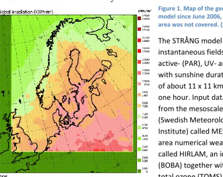
Figure 1. Map of the geographic area covered in the STRÅNG model since June 2006, prior to that the deep green colored area was not covered. (SMHI, u.d.)
The STRÅNG model system produces
instantaneous fields of global-, photosynthetically active- (PAR), UV- and direct radiation together with sunshine duration at a horizontal resolution of about 11 x 11 km and a temporal resolution of one hour. Input data to the model are retrieved from the mesoscale analysis system at SMHI (Swedish Meteorological and Hydrological Institute) called MESAN, a high resolution limited area numerical weather prediction model (NWP) called HIRLAM, an ice model for the Baltic Sea (BOBA) together with satellite measurements of total ozone (TOMS). Before 1 of June 2006 the area coverage was smaller (colored area in Figure 1) and the spatial resolution was about 22 x 22 km. Clear-sky condition is modeled with the spectral clear-sky model SMART2. The output is then
multiplied by a neural network function which captures the influence of clouds and precipitation. The cloud information from MESAN is a synthesis of data from both polar (NOAA) and geostationary (METOSAT) satellites as well as ground based observations. For more information about the STRÅNG model readers are referred to (Landelius, et al., 2001) and (SMHI, u.d.)
Validation
3.1
Table 1 shows the mean validation values for the period 1999 to 2009 at the 12 of the stations in the SMHI radiation network, as presented on the STRÅNG homepage (SMHI, u.d.).
Table 1. Normalized relative MBD, MAD and RMSD at the 12 of the stations in the SMHI radiation network, for the period 1999-2009 (SMHI, u.d.)
Global radiation Direct radiation Hourly MBD -0.2 % -0.4 % Hourly MAD 2.1 % 3.5 % Hourly RMSD 30 % 57 % Daily MBD -0.2 % +0.5 % Daily MAD 2.1 % 3.2 % Daily RMSD 16 % 31 % Monthly MBD +1.3 % +1.3 % Monthly MAD 2.3 % 3.3 % Monthly RMSD 8.9 % 14 %
To validate the model outside Sweden, a study was conducted comparing modeled data from STRÅNG with observed data. Source of for the observed data are The World Radiation Data Centre (WRDC, u.d.), Baseline Surface Radiation Network (BSRN, u.d.) and eKlima (Norwegian
15
3.1.1 Geospatial validation
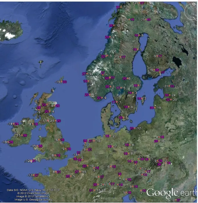
Daily global radiation from the STRÅNG model was compared with observed values; the year 2007 was selected as there was most data available for this year. To visualize the variation due to geographical difference the result was mapped to Google Earth. Figure 2 shows relative MBD and RMSD. The validation data are also available in more detail in Appendix B.1. The maps clearly shows that there the accuracy and bias varies quite much geographically. Sweden got the best result considering both MBD and RMSD. There are some areas (most of central Europe, east England and south of Finland) where the model performs quite well when looking on the RMSD but with a negative bias. Stations near the coast of the Atlantic and North Sea all show high RMSD values and significant negative bias. The Baltic countries and northern part of Finland show the worst result with all stations strongly negatively biased and a RMSD over 30%. High altitude stations also show worse result.
Figure 2. Daily global radiation validation figure, year 2007. Relative MBD represented by white numbers and relative RMSD by purple. All values are in percentage. Note that some labels are overlapping resulting in that all values aren’t visible. The validation data are available in more detail in Appendix B.1.
16
3.1.2 Temporal validation
A few stations were selected for a long term validation. The selection was done based on data availability and with the aim of getting a geographic spread.
Figure 3. Upper: Relative MBD for daily global radiation normalized on yearly basis. Lower: Relative RMSD for daily global radiation normalized on yearly basis. Both: Stations with similar geographical condition (subjectively considering both local conditions and in-between station distance) have same “line appearance” in the figure.
As can be seen in Figure 3 there’s a quite decrease in performance around year 2010, according to Tomas Landelius3 at SMHI there was a problem with the analysis of cloud related parameters for the period 2009 to 2011 (30/3). If this period is not considered it is clear that the Swedish station of Stockholm shows the most consistent and reliable result. Also the Finnish stations of Jokionen and
3 Personal communication, August 28, 2012 0% 5% 10% 15% 20% 25% 30% 35% 40% 45% 50% 1999 2000 2001 2002 2003 2004 2005 2006 2007 2008 2009 2010 2011 2012
Stockholm Helsinki Jokioinen Særheim Praha Wien Lerwick Aberdeen Cabauw De Bilt Toravere
-30% -25% -20% -15% -10% -5% 0% 5% 10% 15% 20% 1999 2000 2001 2002 2003 2004 2005 2006 2007 2008 2009 2010 2011 2012
17
Helsinki shows reasonable consistent result but with an allover negative bias. In about 2005 the bias seems to get more negative, especially for the Central European and British stations.
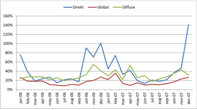
3.1.3 Correlation: direct, global and diffuse
Building simulations software like IDA ICE and EnergyPlus uses the direct and diffuse components of solar radiation. But as there are few source of observed direct radiation the validation was conducted on global radiation. A correlation study was made on a few stations with data available for all three solar radiation components: direct, global and diffuse radiation.
Figure 4. Relative RMSD normalized on yearly basis for direct, global and diffuse radiation for Toravere. Visualizing how the solar radiation components correlate.
Figure 5. Relative RMSD normalized on yearly basis for direct, global and diffuse radiation for Lerwick and Cabauw. As can be seen in Figure 4 and Figure 5 there’s a correlation between RMSD results of the different radiations components. The correlation coefficient for global and direct radiation is 0.90, 0.72 and
0% 10% 20% 30% 40% 50% 60% 70% 1999 2000 2001 2002 2003 2004 2005 2006 2007 2008 2009 2010 2011 2012
Direct Global Diffuse
0% 10% 20% 30% 40% 50% 60% 70% 2000 2001 2002 2003 2004 2005 2006 2007 2008 2009 2010 2011 2012 2013
Cabauw direct Cabauw global Cabauw diffuse
18
0.24 for the stations Toravere, Cabauw and Lerwick respectively. And for global and direct radiation it is 0.37, 0.76 and 0.56 in same order as above.
Figure 6. Relative RMSD normalized on monthly basis for direct, global and diffuse radiation for Norrköping. The Norrköping station was studied by normalizing the RMSD on monthly basis. The correlation coefficient for global and direct radiation is 0.73 for the studied period 2006 to 2007. And for global and diffuse radiation the correlation is 0.43. It can also be seen in Figure 6 that the relative RMSD gets much higher during the winter, which is expected as the monthly mean value used for normalization gets lower during winter leading to a higher relative error.
0% 20% 40% 60% 80% 100% 120% 140% 160% ja n -06 fe b -06 m ar-06 ap r-0 6 m ay -06 ju n -06 ju l-0 6 au g-0 6 se p -0 6 o ct-06 n o v-06 d ec -06 ja n -07 fe b -07 m ar -07 ap r-0 7 m ay -07 ju n -07 ju l-0 7 au g-0 7 se p -0 7 o ct-07 n o v-07 d ec -07
19
“Real-Time Weather Converter”-software
4
As part of this degree project a tool was developed to demonstrate how locally observed weather data can be merged with modeled solar radiation data to create AMY-files. The tool retrieves weather data from Integrated Surface Database (ISD) and modeled solar radiation data from STRÅNG. Supported weather file formats are EnergyPlus EPW and IDA ICE PRN formats. The tool is programmed in C# making use of the .NET Framework. The tool features:
Retrieving data from ISD and STRÅNG databases Data extraction and merging of data
Data editing in tabular form
Interpolation and a fill scheme for missing data
Creation of AMY-weather files, supporting IDA ICE and EnergyPlus weather file formats
Figure 7. Main user interface of the Real-Time Weather Converter tool. Tool version 1.6.
Data retrieval
4.1
Actual metrological data are retrieved from ISD: air dry-bulb temperature, dew point temperature, wind speed, wind direction and atmospheric pressure. ISD consists of global hourly and synoptic observations compiled from numerous sources, into a database supported by The National Climatic Data Center of USA. ISD data have been quality checked by algorithms checking for: proper data format for each field, extreme values/limits, consistency between parameters, and continuity between observations. (National Climatic Data Center, 2012).
3198 stations from the ISD are included, but not all of these stations have enough information to make a useful weather file. There are differences from country to country; stations from some
1. Select ISD station
8. “Additional" data according to WMO resolution 40. For some countries this might make data allowable for commercial use.
2. Select station by WMO number
3. End date for available data according to last update
4. Link to interactive station map 5. Choose dates to retrieve, edit and convert data for
6.Starts retrieving STRÅNG using selected station geographic coordinates. This is time consuming, so be patient
7. Retrieves weather observation data from ISD for selected station
9. Start automatic conversion to IDA ICE or EnergyPlus weather file format.
10. Loads ISD and STRÅNG data for selected period for viewing, editing and conversion to desired format.
20
countries (e.g. Germany) lack recent data while other (e.g. Sweden and UK) have data from most available stations. Stations are very roughly filtered with following criteria’s:
Geographic area (Figure 1 shows area that is included).
Only stations that have data in-between 1999 to current date are included.
Stations with missing information on longitude, latitude, date, WMO-number and FIPS are excluded.
Modeled solar radiation data are retrieved from STRÅNG, see chapter 3 for more details. Figure 7 shows the main user interface of the tool (version 1.6) where the retrieval of data are handled, Figure 8 shows the user interface where the merging and interpolation of data are done and AMY-weather files created. The data are presented as tables and can be copied and pasted, allowing for extraction of data insertion of data from other sources. Data can also be shown as monthly or daily mean values.
Figure 8. User interface for data editing and creation of AMY-weather files.Tool version 1.6.
Data conversion
4.2
Raw data from the ISD and STRÅNG is loaded into the software, adjusted to local time determined by information from selected station. STRÅNG data can be loaded either raw as “on the hour” or shifted (interpolated) half an hour backwards.
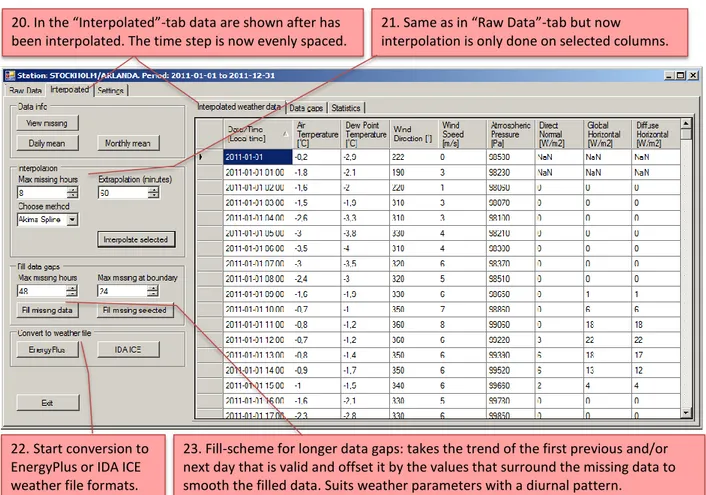
20. In the “Interpolated”-tab data are shown after has been interpolated. The time step is now evenly spaced.
21. Same as in “Raw Data”-tab but now interpolation is only done on selected columns.
23. Fill-scheme for longer data gaps: takes the trend of the first previous and/or next day that is valid and offset it by the values that surround the missing data to smooth the filled data. Suits weather parameters with a diurnal pattern.
22.Start conversion to EnergyPlus or IDA ICE weather file formats.
21
4.2.1 Interpolation
Data gaps are identified and interpolated by selected method. Supported methods are Linear Spline, Cubic Spline and Akima Spline. For the actual interpolation algorithms the open source Math.NET Numerics library is used (Math.NET, 2012).
Interpolation also serves the purpose of getting data to wanted timestamp (re-sampling). For example if you have data for 12:20 and 12:50 (which often is the case for airports) you could interpolate this to 12:00 or to 12:00 and 12:30.
4.2.2 Longer data gaps
If there are longer periods of missing data, these are filled by taking the trend of the first previous or next day that is valid and offset it by the values that surround the missing data to smooth the filled data, see equation (5). A similar method is used by EnergyPlus Real-Time Weather Data website (Long, 2006). The idea is that many meteorological parameters have a diurnal pattern that this method is able to catch thus giving better result than simple interpolation.
( ) ( ) ( ( ) ( ))
(( ( ) ( )) ( ( ) ( ))) (5)
( ) is the time step to fill.
( ) ( ) are the values around the missing data points.
d is the offset back to or forward to previous valid day, that’s a …,-48, -24, 24, 48,… hour offset. n is actual position.
Appendix A.1 shows the C# method used for filling data gaps taking the trend from the previous day. Both forward and backward methods are run and then the result is mixed together to get one final estimate. If one of the forward or backward methods fail due to missing data, the result from the other one is used. Three different methods to mix (and no mixing) the values were tested and the result is presented in Table 2, mixing 50/50 gives the best result and is therefore used in the tool. Hard mixing: ( ) ( ) ( ) ( ) ( ) ( ) (6) Soft mixing: ( ) ( ) ( ) ( ) ( ) (7) 50/50 (linear interpolation):
22
( ) ( ) ( )
(8)
N is the number of missing data points. Table 2. Result from testing different mixing methods. Data gap (hours) N Hard, MBD Soft, MBD 50/50, MBD Non, MBD Hard, RMSD Soft, RMSD 50/50, RMSD Non, RMSD 7-12 10651 0.0% 0.0% 0.0% -0.1% 20.19% 19.75% 19.3% 20.9% 13-24 17375 -0.5% -0.4% -0.3% -0.2% 27.8% 27.0% 26.3% 30.6% 25-48 25075 -1.3% -1.3% -1.1% - 41.1% 38.3% 37.8% - 49-72 19540 0.8% 0.8% 0.9% - 55.6% 52.2% 47.8% -
4.2.3 Testing interpolation and fill schemes
Three interpolation schemes from the Math.NET Numerics (Math.NET, 2012) open source library were tested: Linear, Cubic and Akima Spline. Also the fill-scheme described in chapter 4.2.2 was tested. Figure 9 shows graphically how the different schemes fill data gaps of 7 to 12 hours.
Figure 9. Missing data point filled by different interpolation and fill scheme methods. Data gaps are 7 to 12 hours. Original data is air dry-bulb temperature from springtime 2007 Stockholm/Arlanda.
Date used for the test was air dry-bulb temperature for Stockholm-Arlanda for the period 2007 to 2011. The testing was done by estimating artificial created data gaps, which were randomly distributed over the dataset so that there was 25-28 hour of real data between the gaps, following Mathlab function was used for the purpose:
function [Out,NaNs]= FillWithNaNs(Table,n1, n2) Out=Table; i=2; NaNs=0;
while i<43824-(n2+3)
% random number between n1 and n2
r=round(n1 + (n2-n1) * rand(1)); Out(i+1:i+r)=NaN; i=i+r; 0 5 10 15 20 25 Tem p e ratu re ( ˚C) Time (hour) Linear Cubic Akima Fill Real temp
23
NaNs=NaNs+r;
% random number between 25 and 28
r=round(25 + (28-25)*rand(1)); i=i+r;
end end
Table 3 shows result of the first test, where data gaps are randomly selected between specified intervals. In Table 4 data gaps are not varied in size, the purpose is to find the limits where different schemes give best result. The result implicate that the Akima Spline interpolation is best suited for temperature data gaps in the interval 2 to about 8 hours. For gaps of about 9 to 48 hours the fill scheme clearly gives best result. For gaps between 2 and 5 days the fill scheme will still give slightly better result than simple linear interpolation. As the fill scheme will preserve the diurnal
characteristics of meteorological parameters, e.g. temperature, it will most likely give a more accurate result when used for dynamic building simulations than linear interpolation. Table 3. MBD and RMSD for different schemes tested on artificially created data gap intervals
Data gap (hours) N Linear, MBD Cubic, MBD Akima, MBD Fill, MBD Linear, RMSD Cubic, RMSD Akima, RMSD Fill, RMSD 2-6 4512 0.4% 0.5% 0.5% 0.5% 12.1% 11.6% 10.7% 12.3% 7-12 10651 0.1% 0.0% 0.1% 0.0% 24.8% 21.4% 19.6% 20.2% 13-24 17375 -1.2% -0.4% -0.9% -0.5% 46.6% 46.2% 42.7% 27.8% 25-48 25075 -1.6% -2.6% -2.0% -1.3% 50.7% 99.4% 63.0% 41.1% 49-72 19540 -2.0% -7.5% -2.6% 0.8% 55.9% 153.7% 88.8% 55.6% 73-96 33207 1.1% -3.7% -0.6% -0.9% 56.2% 198.1% 107.8% 52.6% 97-120 35200 -3.5% - - -0.7% 58.7% - - 58.9% 121-144 36442 -2.0% - - 5.1% 62.1% - - 64.2%
Table 4. MBD and RMSD for different schemes tested on artificially created data gaps. Data gap (hours) N Linear, MBD Cubic, MBD Akima, MBD Fill, MBD Linear, RMSD Cubic, RMSD Akima, RMSD Fill, RMSD 2 1594 0.1% 0.1% 0.1% 0.1% 6.5% 6.7% 6.2% 6.5% 3 3074 -0.4% -0.4% -0.3% -0.4% 8.1% 8.7% 7.7% 8.9% 8 10152 - - -0.5% -0.6% - - 18.5% 18.7% 9 10168 - - 0.0% 0.1% - - 18.6% 18.0% 11 12010 - - 0.0% -0.3% - - 22.5% 21.3% 4.2.4 Time shift
STRÅNG values are in irradiance [W/m2], with other words instantaneous, and refer to the full hour (Landelius, et al., 2001). For weather data files used in building simulation software time integrated irradiation [Wh/m2] values are used: amount of solar radiation during the number of minutes preceding the time indicated (EnergyPlus, 2011). In other words the value for 14.00 o’clock refers to the average value of the interval from 13.00 to 14.00 o’clock.
If trapezoidal integration is applied, and linear interpolation is used for getting the ( ) term, it will turn out as a simple linear interpolation as can be seen in equation (9).
24
( ) ( ) ( ( ) ( ) ( )) ( ) ( ( ) ( ( ) ( )) ( )) ( ) ( ) ( )
(9)
The effect of the time shift was tested on hourly global data from Wien Hohe Warte for the year 2007, source WRDC. The relative MBD was not affected by the time shift, relative RMSD changed from 41.9 % to 36.3 %, the relative RMSD between shifted and unshifted (on the hour) STRÅNG data was 27.0 %. Also using Akima Spline interpolation instead of linear interpolation in equation (10) was tested, but did not give better result than linear interpolation. Table 5 shows the result as the correlation between the tested methods.
Table 5. Correlation values of tested methods Measured WRDC STRÅNG On the hour STRÅNG Shifted (linear) STRÅNG Shifted (Akima) Measured WRDC 1 STRÅNG On the hour 0.9675 1 STRÅNG Shifted (linear) 0.9754 0.9864 1 STRÅNG Shifted (Akima) 0.9754 0.9864 0.9999 1 4.2.5 Diffuse radiation
At present STRÅNG provides direct and global radiation, the diffuse horizontal radiation needed for energy simulations is calculated by using the equation (10).
( ) (10)
The elevation of the sun is calculated from information about the local time, longitude and latitude. Appendix A.2 shows a part of the C# method used to calculate diffuse horizontal irradiation, also the linear interpolation to shift solar data with a half hour is included in that code sample. There will be some error introduced at this point due to difference in methods for calculating the solar elevation. The STRÅNG model does model the diffuse irradiance parameter as well but it’s not available at the data extraction webpage at present time.
4.2.6 EnergyPlus and IDA ICE weather files
When data have been interpolated to right timestamp (re-sampled) and data gaps are filled, conversion to EnergyPlus or IDA ICE weather files format is possible. For conversion to EnergyPlus EPW file format the library file EPlusWth.dll supplied by EnergyPlus is used. Conversion to IDE ICE PRN file format is done in the software. To calculate the relative humidity from dry-bulb and dew point temperature following C# code, based on the Clausius-Clapeyron equation, is used:
public static double Humidity(double T, double Tdp) {
25
// T = dry-bulb temperature in Celsius // Tdp = dew-point temperature in Celsius
double E = 6.11 * Math.Exp(5417 * (0.003653 + 1 / (Tdp + 273.15))); double Es = 6.11 * Math.Exp(5417 * (0.003653 + 1 / (T + 273.15))); double RH = (Es / E) * 100;
if (RH > 100) return 100; else if (RH < 0) return double.NaN; else
return Math.Round(RH, 1); }
26
Weather data impact and uncertainty
5
In Nordic countries outdoor air temperature is the most important factor for common building energy simulations, but during summertime solar radiation has an equal influence (Jylhä & et.al., 2011). Other parameters like humidity, atmospheric pressure and wind have much smaller impact on the simulation result and therefore only temperature and solar radiation were studied.
Temperature
5.1
Long timeseries of monthly mean temperatures were extracted from the ISD using the Real-Time Weather Converter tool. Figure 10 shows the monthly and yearly mean temperatures and 2* Standard Deviation (SD) for selected stations for the period 1981-2010. For northern stations Kevo-Utsjoki, Stockholm and Tartu-Toravere the yearly SD is around 1˚C which is in line with what Lars Jensen’s study (Jensen, 2010) resulted in using temperature data from 25 Swedish stations. These northern stations also show the large monthly variation, especially for winter months. For the southernmost stations Payerne, Camborne and Cabauw the yearly SD is much lower (0.5 to 0.8 1˚C) and the monthly variation smaller.
A SD of 1˚C means that in two of three years the mean temperature will be in the interval Tmean ± TSD.
Using Tmean ± 2*TSD gives the mean temperature interval with a 95 % confidence, assuming normal
distribution around the mean value. With other words: to predict the mean temperature for January for Tartu with a 95 % confidence would give -4.5 ± 8.2˚C, assuming normal distribution around the mean value (which is not the case as the Skewness is -1.56 and Kurtosis is 2.28 indicating a long and thin left tail in the distribution). While predicting January mean temperature for the coast near Camborne with 95 % confidence would give 6.9 ± 3 ˚C, again assuming normal distribution (which is almost the case with Skewness of -0.9 and Kurtosis of 0.1)
Appendix B.2 contains more descriptive statistics in tabular form for the selected stations. From this table more trends can be seen. For example Skewness tends to be positive (right tailed) during summer months and negative (left tailed) during winter months for all stations. This indicates that there are winters when the mean temperature drops much under the mean and summers when the mean temperature is much higher than the long term mean.
The outdoor temperature (or more exactly the difference between outdoor and indoor temperature) is the driving force for heat transfer occurring in a building, and therefore outdoor temperature is one of the parameters having the strongest impact on a dynamic building energy simulation. How strong the impact is depends on what kind of building that is being modeled and of course of the outdoor temperature itself. For example a residential house with low internal gains and high
envelope area volume ratio (Aenvelope/Vbuilding) the outdoor temperature will have large impact while a
large commercial building with high internal gains and low envelope area volume ratio the impact will be relatively smaller.
27
Figure 10. Monthly and yearly mean temperatures (circles) and 2*standard deviations (bars) for the period 1981-2010.
Solar radiation
5.2
Using measured solar radiation data from the BSRN, extracting monthly means using the PANGAEA web portal (PANGAEA, u.d.), a study was made on a few stations with longer period of data. Figure 11 to Figure 15 shows the result as error charts giving the monthly mean and 2*SD values for all three radiation components. The period studied is constrained to data availability and differs from station to station, therefore making comparisons between stations problematic. Appendix B.3 contains a more detailed table with descriptive statistics for selected stations.
It can clearly be seen from the figures that the variation is much smaller for diffuse than for direct radiation. The yearly SD for studied stations is in the range 1.0 to 1.9 W/m2 for the diffuse radiation and 5.0 to 17.9 W/m2 for the direct radiation component, given in Relative Standard Deviation (RSD)
28
the values are 1 % to 4 % and 5 % to 9 %. In absolute values the SD is larger for summer month, as expected as solar radiation is stronger during summer. But the relative SD (RSD) is actually slightly larger for winter months, as can be seen in Figure 11 showing RSD for the direct radiation
component.
Figure 11. Monthly and yearly mean direct radiation RSD.
To predict the mean July direct radiation for Tartu with a 95 % confidence would give 223 ± 114 W/m2. While on yearly basis the direct radiation for Tartu can be predicted as 120 ± 11 W/m2 with 95 % confidence. With other words uncertainty is high on monthly basis while the yearly mean radiation don’t vary that much.
Looking at Skewness and Kurtosis for all studied stations indicates that the solar fits a normal distribution reasonable well, even though a slight tendency to negative Kurtosis on yearly basis for direct radiation can be seen indicating that the observation cluster less and have thicker tails until the extreme values of the distribution.
0% 10% 20% 30% 40% 50% 60% 70%
Jan Feb Mar Apr May Jun Jul Aug Sep Oct Nov Dec Year
29
Figure 12. Monthly and yearly mean solar radiation (circles) and 2*standard deviations (bars). Tartu-Toravere 1999-2011.
30
Figure 14. Monthly and yearly mean solar radiation (circles) and 2*standard deviations (bars). Cabauw 2005-2012.
Figure 15. Monthly and yearly mean solar radiation (circles) and 2*standard deviations (bars). Payerne 1993-2009. Impact of solar radiation on dynamic building simulation depends on what kind of building (i.e. window area, solar energy applications, building heat capacity) is being modeled and at what outdoor temperature the solar radiation occurs. Depending on the outdoor temperature the solar radiation either contributes to the heating of the building, cause need for cooling or neither. Figure 16 shows the cumulative sum of yearly irradiation as a function of temperature for three selected sites.
31
Figure 16. Cumulative sum of yearly irradiation [kWh/m2] as a function of temperature. Based on data for the period 2006-2007.
Testing on an IDA ICE model
5.3
The IDA ICE model used for testing is based on a three story 1450 m2 office building located in Västerås, Sweden. The building was built in 1982 and renewed in 1990 and is quite typical Swedish office building with energy consumption in the lower end compared to other Swedish offices. It has district heating, air-to-air cooling, central ventilation with heat recovery and 60 h/week operation time. The building and the model is described in more detail in the report “Energy simulation of a mid-sized office building” (Lundström, 2012).
Table 6. Comparison between climate files. The relative difference towards the TMY-file is given in the brackets. Weather file Air
tempera-ture [˚C] Relative humidity [%] Direction of wind [deg] Wind speed [m/s] Direct radiation [W/m2] Diffuse radiation [W/m2] TMY Stockholm (Arlanda), ASHRAE 6.5 78 - - 89 59 Stockholm-77 (Bromma) 6.2 (-5%) 78 178 3.3 106 (20%) 58(-3%) AMY-2010 Stockholm (Arlanda) 5.1 (-22%) 81 192 3.1 131 (47%) 46 (-22%) AMY-2011 Stockholm (Arlanda) 7.8 (20%) 79 202 3.4 135 (52%) 56 (-5%) AMY-2010 Västerås 4.6(-29%) 80 186 3.0 113 (27%) 48 (-17%) AMY-2011 Västerås 7.5 (15%) 76 200 3.6 120 (36%) 58 (-2%)
IDA ICE provides two weather files for Stockholm (about 80 km east of Västerås). A TMY based on weather data from Arlanda airport, source being ASHRAE IWEC weather files which are the same files
32
that are provided by EnergyPlus. And a so called typical reference year weather file for Bromma airport, the reference year being 1977. Four AMY-files were made with the Real-Time Weather Converter tool, for the years 2010 and 2011. Table 6 shows mean yearly values for the weather parameter in the files. From the STRÅNG-model validation chapter 3.1 it’s clear that the model has a slight negative bias (especially for year 2010), so the real solar radiation will much likely be
somewhat larger than presented in the table. Note that the ASHRAE IWEC TMY weather file has a very low direct radiation value. It’s clearly some fault with this file, Chapter 6 studies the IWEC weather files in more detail.
Table 7. Comparison of results from simulations with different climate files. The relative difference towards the TMY-file is given in the brackets.
Electricity for cooling [kWh/m2] Total electricity [kWh/m2] District heating [kWh/m2] Total energy Consumption [kWh/m2] TMY Stockholm (Arlanda), IWEC 5.4 67.9 61.3 129.2 Stockholm-77 (Bromma) 5.5 (1.9%) 67.8 (-0.1%) 60.1 (-2.0%) 127.9 (-1.0%) AMY-2010 Stockholm (Arlanda) 7.3 (35.2%) 69.6 (2.5%) 71.4 (16.5%) 141.0 (9.1%) AMY-2011 Stockholm (Arlanda) 8.0 (48.1%) 70.3 (3.5%) 51.6 (-15.8%) 121.9 (-5.7%) AMY-2010 Västerås 6.0 (11.1%) 68.3 (0.6%) 74.4 (21.4%) 142.7 (10.4%) AMY-2011 Västerås 7.2 (33.3%) 69.5 (2.4%) 53.1 (-13.4%) 122.6 (-5.1%)
Table 7 shows results from simulations with different climate files. If we look at the simulations done with the TMY and Stockholm-77 weather file we can see that the heating need is slightly less for Stockholm-77, which most likely is caused by the slightly lower mean temperature. But the cooling need is higher which most likely is caused by the lower mean solar radiation for the TMY file. The differences in result for the AMY-file vs. the TMY-files are large, which to most extent can be deduced to the fact that the year 2010 was an unusually cold year and 2011 was an unusually warm year. Comparing result from the “AMY-2011 Västerås”-file with the “AMY-2011 Stockholm”-file shows that heating demand was 3% higher and the cooling need 10% lower for Västerås. This shows the impact the weather has, as the yearly mean temperature was 4% lower and the yearly mean solar radiation was 10 % lower in the “AMY-2011 Västerås”-file. The total energy consumption, however, stays quite the same as the two weather parameters in this case work in different directions.
It’s difficult to draw general conclusion of the impact on the energy consumption from climate parameters as they are interlinked and impact energy consumption in many ways depending on circumstances. Impact will vary for building to building depending on design, location and season.
33
ASHRAE IWEC weather files
6
The building simulation software IDA ICE and EnergyPlus provides so called IWEC4 (International Weather for Energy Calculations) weather files and were produced by AHRAE in 2000. These are TMY-files derived from up to 18 years of hourly weather data. The weather data are supplemented by solar radiation estimated on an hourly basis from earth-sun geometry and hourly weather elements. (EnergyPlus, 2011).
The radiation components of the IWEC files were compared against STRÅNG data because observed direct radiation data sources are rare. Sites that are selected for the comparison are stations that showed good bias- and RMSD-values in the validation made in Chapter 3.1. Comparison against observed BSRN radiation data was also done for two sites, and also against the TRY2012 file for Helsinki-Vantaa.
Table 8. Comparison of ASHRAE IWEC weather files yearly mean radiation with radiation from STRÅNG and BSRN. *1 BSRN data for Paris-Palaiseau 2004-2006. *2 BSRN data for Lindenberg 1995-2005, 50 km east of berlin. *3 TRY2012 for Helsinki-Vantaa (Jylhä, et al., 2011). *4 This weather file don’t include all diffuse radiation (Jylhä, et al., 2011)
Site Difference ASHRAE STRÅNG 2007 STRÅNG
global MBD Direct Diffuse Direct Diffuse Direct Diffuse
Stockholm -33% 5% 88.9 59.6 132 57 1% Helsinki -26% 16% 81.3 64.7 110 56 -8% Göteborg -28% 12% 84.3 66.3 117 59 -1% Karlstad -20% 10% 107 58.2 134 53 -5% Östersund -26% 6% 88.9 58.2 120 55 -1% Paris-Orly -25% 3% 77.5 76.3 103 74 -5% Oostende -17% -5% 85.1 69.5 103 73 -2% Berlin -24% -6% 80.3 66.8 105 71 Wien -30% -12% 93.1 71.6 133 81 5% Hamburg -22% 7% 70.6 69.7 91 65 -3% Aberdeen -37% 17% 55.1 70.3 87 60 -8%
Site Difference ASHRAE Other STRÅNG
global MBD Direct Diffuse Direct Diffuse Direct Diffuse
Paris-Orly*1 -39% 3% 77.5 76.3 127 74 -5%
Berlin*2 -27% 3% 80.4 66.9 110 65 -9%
Helsinki*3 -37% 32%*4 81.3 64.7 129 49
Table 8 shows the result from the comparison. Recall the STRÅNG validation in Chapter 3.1 that showed that STRÅNG data also are somewhat negatively biased. STRÅNG data are only validated against global radiation but as result presented in chapter 3.1.3 demonstrates there is a strong correlation between errors occurring in STRÅNG global and direct radiation data. The STRÅNG data are only for one year while the IWEC is TMY file constructed from 18 years of data which also affects the result. The comparison against BSRN data is more reliable and shows even higher negative bias.
4
Note that there exist also a newer set of files called IWEC2 that can be purchased from ASHRAE, these files seems not to be systematically biased for North Europe but haven’t been studied in this paper. See Chapter 8 for a short description of the IWEC2.
34
Taking all above mentioned in consideration it’s apparent that the IWEC files direct solar radiation component has a strong negative bias, roughly ranging in-between 20 to 40 % for selected sites.
35
Conclusions
7
The main conclusion is that solar radiation data from the STRÅNG modeling system are suitable for calibration of building simulation models. For some areas the data would also be suitable for creation of TMY-files and for other energy engineering applications.
For Sweden STRÅNG data are accurate and have low bias, both in long term and geospatially.
Outside of Sweden the STRÅNG accuracy is in general poorer and bias higher. There exist some sites (mainly in Central Europe) with reasonable good result for some time periods but the result isn’t as consistent in long term as for Sweden.
It’s difficult to draw general conclusion of the impact on the energy consumption from climate parameters as they are interlinked and impact energy consumption in many ways depending on circumstances. Impact will vary for building to building depending on design and location. Weather data uncertainty is, however, easier to study:
Uncertainty, expressed as SD, in yearly mean temperature is about 1˚C for the Nordic countries. The SD gets smaller for sites at more southern latitudes and for coast-neat sites: 0.6 ˚C for Payerne, Switzerland, and 0.5 ˚C for Camborne, UK.
On monthly basis the variation in mean temperature is much stronger, especially for
northern and inland sites. The Nordic countries mean temperature SD ranges from 3.5 to 4.7 ˚C for the winter months, while the summer months are more consistent with SD in the range of 1.3 to 1.9 ˚C. The same pattern is visible in site at more southern latitudes but with much lower variation, the cost near Camborne has a SD of 0.7 to 1.7 ˚C on monthly basis. Mean direct irradiance SD for studied sites ranges from 5 to 19 W/m2 on yearly basis. While
on monthly basis the SD ranges from 40 to 60 W/m2 for summer months. However the
sample base was small and of inconsistent time periods and the numbers can only be seen as indicative.
The fill scheme described in Chapter 4.2.2 is a fairly straight forward approach for dealing with longer data gaps and gives reasonable good result. A few longer data gaps will not affect the quality of the data too much if the data are to be used for model calibration against utility bills (usually done on monthly or daily basis).
The fill scheme performs significantly better than interpolation for data gaps (outdoor temperature) of about 9 to 48 hours. For example the 25-48 hour gap test with fill scheme in Table 3 has 57 % of its temperature data taken away but still the average temperature of 6.99 ˚C for the whole period is just affected by -0.053 ˚C.
For gaps between 2 and 5 days the fill scheme will still give slightly better result than linear interpolation.
Akima Spline interpolation performs better than linear interpolation for data gaps (outdoor temperature) in the interval 2 to about 8 hours.
The commonly used and freely available IWEC files direct radiation parameter has a very strong negative bias of about 20 to 40 % for Northern Europe. These files should be used with care, especially if solar radiation has a significant impact of on the building being modeled.
36
Discussion
8
The use of ISD data outside of the US might be restricted with respect to the WMO Resolution 40, quoting the NOAA Policy:
“The following data and products may have conditions placed on their international commercial use. They can be used within the U.S. or for non-commercial international activities without restriction. The non-U.S. data cannot be redistributed for commercial purposes. …” (NOAA, 2012)
Norway, Spain, Netherlands, Slovenia, UK (ECOMET, u.d.) and soon Sweden (Morus konsult AB, 2012) are European countries that have similar unrestricted data policy to that of US NOAA. Other
European countries do however restrict (to varying degree) the usage of their weather data. As long as ISD data are utilized the resulting AMY-files should be used for research, education, and other non-commercial activities. It is possible to insert data from other sources or from own local measurements and then the resulting weather files can be used for commercial purposes.
Validation of the STRÅNG model system shows some inconsistence in accuracy outside of Sweden, both in temporal and geospatial dimension. If these issues would be addressed it would be a very interesting source of modeled solar radiation data to be used for different kinds of energy
engineering applications, requiring better quality on solar radiation data than calibration of building simulation models does.
There are now IWEC2-files available from ASHRAE, covering over 3000 international stations. The underestimation (for direct solar radiation) present in the old IWEC-files is not present in the IWEC2-files for Stockholm and Helsinki5. Both the old IWEC and IWEC2 used the Zhang-Huang model that derives global horizontal solar radiation from cloud cover, change in dry-bulb temperature over the past three hours, relative humidity, wind speed and a set of regression coefficients. In the old IWEC a single set of regression coefficients where derived using measured solar data for two Chinese cities. In IWEC2 Köppen-Geiger climate classifications was used to group IWEC2 stations, using different sets of regression coefficients for the Köppen-Geiger zones. Also a new model for splitting the global horizontal to diffuse and direct normal solar radiation was used in the IWEC2-files.6
Deviation in STRÅNG values correlate quite well with nearness to ocean (UK, Norway and west coast of Europe) and altitude (e.g. stations Poprad-Ganovce, Sonnblick and Löken i Volbu). Also vicinity to mountains seems affect the STRÅNG model system negatively, e.g. Norwegian station Kise. The strong underestimation at the Baltic stations is harder to explain as caused by climate differences, the Baltic climate don’t deviate that much from the Swedish. The same goes for the two north Finnish stations. This deviation at the Baltic and North Finnish stations need to be studied further. Apart from the Baltic and North Finnish stations it seems very likely that adding one more input parameter, describing the local climate/geography, to the STRÅNG “cloud function” would be
5
Personal communication, November 8, 2012, with Joe Huang contractor of the IWEC2 project. Reference:
AMY-weather files for North Europe. [Discussion Group]. Available at:
http://tech.groups.yahoo.com/group/EnergyPlus_Support
6
37
beneficial for the STRÅNG model accuracy. The “cloud function” would also then need to be trained (tuned) with solar data from stations outside of Sweden, so that all types of climate present in the area covered by STRÅNG would be represented. For example a station at the Norwegian west coast would most likely also represent the climate (from cloud formation point of view) of the west coast of France, or at least does it better than a Swedish station do.
This paper has focused on creation of AMY-weather files. As the time span of the STRÅNG database is growing (soon reaching 13 years) it would be possible to use a similar approach for creating TMY-weather files with a good coverage rate of the urban and semi urban parts of North Europe.
38
References
BSRN, n.d. Baseline Surface Radiation Network. [Online] Available at: http://www.bsrn.awi.de/
[Accessed 9 2012].
ECOMET, n.d. ECOMET. [Online]
Available at: http://www.ecomet.eu/index.php [Accessed 24 10 2012].
EnergyPlus, 2011. Auxiliary EnergyPlus Programs, s.l.: Ernest Orlando Lawrence Berkeley National Laboratory.
Höglund, I., Girdo, V. & Troedsson, C. G., 1985. Solinstrålningstabeller för helklara, halvklara och mulna typdagar, Stockhom: Inst. för byggnadsteknik, Kungliga Tekniska Högskolan.
Huang, J., n.d. (under review) ASHRAE Research Project 1477-RP. s.l.:s.n. Jensen, L., 2010. Utetemperaturens osäkerhet. Lund: Lunds tekniska högskola.
Jylhä, K. & et.al., 2011. Rakennusten energialaskennan testivuosi 2012 ja arviot ilmastonmuutoksen vaikutuksista, Helsinki: Ilmatieteen laitos.
Jylhä, K., Kalamees, T., Tietäväinen, H. & Ruosteenoja, K., 2011. Rakennusten energialaskennan testivuosi 2012 - ja arviot ilmastonmuutoksen vaikutuksista, Helsinki: Finnish Meteorological Institute.
Landelius, T., Josefsson, W. & Persson, T., 2001. A system for modelling solar radiation parameters with mesoscale spatial resolution, Norrköping, Sweden: SMHI.
Long, N., 2006. Real-Time Weather Data Access Guide, Colorado: NREL.
Lundström, L., 2012. Energy simulation of a mid-sized office building, Västerås: Mälardalens högskola. Math.NET, 2012. Math.NET Numerics. [Online]
Available at: http://numerics.mathdotnet.com/ [Accessed 8 2012].
Morus konsult AB, 2012. SMHI öppnar data – intervju med Marcus Flarup. [Online] Available at: http://morus.se/2012/10/smhi-oppnar-data-intervju-med-marcus-flarup/ [Accessed 24 10 2012].
National Climatic Data Center, 2012. Integrated Surface Database. [Online] Available at: http://www.ncdc.noaa.gov/oa/climate/isd/index.php
[Accessed 8 2012].
NOAA, 2012. WMO Resolution 40 NOAA Policy. [Online]
Available at: http://cdo.ncdc.noaa.gov/pls/plclimprod/poemain.accessrouter?datasetabbv=DS3505 [Accessed 24 9 2012].
39 Norwegian Meteorological Institute, n.d. eKlima. [Online] Available at: eklima.met.no
[Accessed 9 2012].
PANGAEA, n.d. PANGAEA - Data Publisher for Earth & Environmental Science. [Online] Available at: http://www.pangaea.de/
[Accessed 2012].
Peel, M., Finlayson, B. & McMahon, T., 2007. Updated world map of the Köppen-Geiger climate classification, s.l.: Hydrol. Earth Syst. Sci 11, 1633-1644..
SMHI, 2011. Normalårskorrigering under vår, sommar och höst med SMHI Graddagar. [Online] Available at:
http://www.smhi.se/Professionella-tjanster/Professionella-tjanster/Fastighet/normalarskorrigering-under-var-sommar-och-host-med-smhi-graddagar-1.18575 [Accessed 22 10 2012].
SMHI, n.d. STRÅNG - a mesoscale model for solar radiation. [Online] Available at: http://strang.smhi.se/
[Accessed 8 2012].
WRDC, n.d. The World Radiation Data Centre (WRDC). [Online] Available at: http://wrdc.mgo.rssi.ru/