The value of time from subjective data on life satisfaction and job satisfaction:
An empirical assessment
Gunnar Isacsson* Anders Karlström** Jan-Erik Swärdh*** April 21, 2008 AbstractThis paper compares estimates of the value of commuting time, working time and household working time from empirical models of subjective assessments of life satisfaction and job satisfaction, respectively, to the corresponding estimates obtained from an empirical search model of the labour market. The results indicate that all three variables produce rather high estimates of the value of commuting time. The results regarding the value of working time differ more between the different outcome variables and it is only significantly different from zero in the model of life satisfaction. Perhaps less surprisingly, the estimate of the value of household working time is also only significantly different from zero in the model of life satisfaction in contrast to the models of job satisfaction and job durations where it is insignificantly different from zero.
*
National Road and Transportations Research Institute, P.O. Box 760, S-781 27 Borlänge, Sweden, email:
gunnar.isacsson@vti.se
**
KTH Stockholm, Sweden, email: andersk@infra.kth.se
***
National Road and Transportations Research Institute, P.O. Box 55685, S-171 06 Stockholm, Sweden, email: jan-erik.swardh@vti.se
1. Introduction
In recent years the use of data on happiness, subjective well-being or life satisfaction has increased in economics (see Layard, 2005, or Frey and Stutzer, 2002, for references).1 Van Praag and Baarsma (2005) suggest, for example, that such data may be useful to estimate economic trade-offs that are relevant for public policy. More specifically, they estimate the economic trade-off between money and airport noise. Frey et al. (2004) argue along similar lines and demonstrate the usefulness of similar data to estimate the value of public goods. The basic idea of these papers is that answers to questions on subjective well-being (life satisfaction) correlate with the experienced utility of respondents.2 In other words, data on subjective well-being may be useful to estimate economic trade-offs that are central to investment in the transport infrastructure and public policy in general.
A potential limitation of this approach is, however, that such estimates may suffer from some kind of ‘subjective bias’. In economics real choices and observed actions are usually considered the primary source of information on preferences, and actions are not necessarily correlated with subjective reports on well-being. In other words, although some aspect of life may have a negative effect on reported well-being it is not certain that the individual is prepared to pay the monetary costs needed to change this aspect of life. Thus, it may be informative to compare estimates of economic trade-offs from data on subjective well-being to those obtained from real choices to assess the usefulness of data on subjective well-being to estimate economic trade-offs.
The basic purpose of the present paper is therefore to produce such a comparison. We focus primarily on the trade-off between commuting time and money.3 The estimates are obtained from data on subjective assessments of life satisfaction and job satisfaction which we compare to those
1
One reason for economists’ previous scepticism regarding the use of data on happiness or subjective well-being has been the potential problem of interpersonal comparisons of subjective well-being.
2
We will use the terms ‘subjective well-being’ and ‘life satisfaction’ interchangeably in the paper.
3
Blanchflower and Oswald (2007) provide a different type of validation study that pertain to cross-country differences in subjective reports of well-being (or happiness) building on the inverse relationship between blood-pressure and psychological well-being. They find that happier nations tend to report fewer blood-pressure problems.
obtained from duration data on job spells.4 To this end we use a data set, the Swedish Level of Living Survey (Eriksson and Åberg, 1987, and Fritzell and Lundberg, 1994), containing all three variables.
The reason for using job durations is the idea outlined by Gronberg and Reed (1994) who suggest that compensating wage differentials for job attributes may be obtained in empirical search models.5 They argue that whenever individuals search for new jobs to improve their situation in the labour market, static wage equations may produce seriously biased estimates of compensating wage differentials (see also Hwang et al., 1998). An empirical search model is, instead, based on a relationship between the hazard rate and the various job attributes including the wage rate. Thus, jobs characterized by higher wages and shorter commuting times will tend to survive longer than other jobs. This conclusion is corroborated by the results in van Ommeren et al. (2000) and Isacsson and Swärdh (2007) where wages tend to correlate positively and commuting time tend to correlate negatively with job durations in the Netherlands and Sweden, respectively. This is the primary motivation for the focus of this paper on job durations as the outcome of observed actions.
Related to our investigation are also the papers by Stutzer and Frey (2004) and Böckerman and Ilmakunnas (2006) who use data on life satisfaction and job satisfaction, respectively, to test the theory of compensating wage differentials. More specifically, they investigate whether labour markets compensate workers for commuting time and work-related disamenities through higher wages.6 The idea of these papers is that if wages compensate for work-related disamenities, job-attributes like noise and commuting should not be correlated with the level of life satisfaction/job satisfaction. Both papers reject this conclusion from the theory of compensating wage differentials, since commuting time and work-related disamenities reduce individuals’ life satisfaction and job satisfaction, respectively. However, in contrast to the suggestion by Gronberg and Reed (1994) and
4
Hensher and Brewer (2001) note that usually some 70 percent of total user benefits of investments in the transport infrastructure are related to time savings.
5
See Rosen (1986) for an earlier survey of research on compensating wage differentials.
6
the approach taken in the present paper, Stutzer and Frey (2004) and Böckerman and Ilmakunnas (2006) both rely on a static wage-equation framework of the labour market.7
We also test the models in a number of ways to see whether the estimated models produce ‘reasonable’ results. First, we include time devoted to other activities in the model, such as working and working in the household, to assess whether the empirical models produce reasonable relationships between life and job satisfaction and time use.8 Secondly, we expect commuting time and working time to be related to both life satisfaction and job satisfaction but household work should probably have no major effect on job satisfaction. Furthermore, an important issue for cost-benefit analyses regarding investments in the transport infrastructure concerns potential geographic differences in the value of commuting time. Since commuting may be more stressful in cities due to congestion, the required wage compensation for commuting may also be higher in cities. We therefore also investigate this issue.
The rest of this paper is organized as follows. Section 2 outlines a theoretical framework and the associated empirical frameworks for estimating the value of time. Section 3 presents the data. Results are presented in section 4 and section 5 concludes.
2. Theoretical and empirical framework
We define an individual’s utility function (u) over goods (G), leisure (L), hours of commuting time (C), working hours (H) and hours of work in the household (D):
)
(
G L C H D u U = , , , , . (U1) 7Ahn (2007) presents an analysis that includes the effect of commuting time on life satisfaction and job satisfaction in a sample of Spanish workers. His results indicate negative effects of commuting time on life satisfaction and negative although weaker effects on job satisfaction. He does not, however, relate these results to data from a model of revealed preferences.
8
Interest in the effect of working hours on life satisfaction is by no means a novelty of the present paper. A number of papers include hours of work as a control variable in the model for life satisfaction (see, for example, Clark, 1997) and a number of papers investigate the relationship between part-time work and life satisfaction (see for examples Booth and van Ours, 2007, and therein for further references).
We assume that goods consumption equals wage earnings; that is, G=wHwhere w denotes the after tax hourly wage rate. There is also a maximum amount of time available to allocate between the four time consuming activities; τ =L+C+H +D where τ is the maximum amount of time. We expect that commuting time and hours of work are perceived as ‘bads’ that need to be compensated through the wage rate.
Assume, furthermore, that the individual continuously search for new jobs and that job offers arrive exogenously from some distribution.9 Here jobs are characterized in terms of wage earnings net of tax, working hours and commuting time (cf. Gronberg and Reed, 1994). The individual chooses to change job if the utility associated with the job offer is larger than the utility associated with the current job. Hence, we expect that the individual will tend to stay longer on the current job the higher are wage earnings, the lower is commuting time and the lower are the hours of work. In other words, the individual will tend to be more satisfied with his/her life and job the higher are wage earnings, the lower is commuting time and the shorter are the hours of work. Furthermore, conditional on w, H and C, the individual chooses the time devoted to household work (D). This choice may be subject to individual restrictions resulting from negotiations in the household.
The value of commuting time (VoCT) is defined as the marginal rate of substitution between commuting time and goods consumption or wage earnings; that is,
( )
wH U C U G U C U VoCT ∂ ∂ ∂ ∂ = ∂ ∂ ∂ ∂ = / / / / .The value of working hours (value of household work) is defined correspondingly as the marginal rate of substitution between hours of work (hours of household work) and wage earnings.
9
It is worth noting an alternative to assuming that jobs are characterized by w, H and C, and that is to assume that they are only characterized in terms of w, and C only, If we also assume that the individual chooses H optimally, conditional on w, and C, we would have the conventional approach of modelling the supply of working hours in a static framework. In this case the value of working time will simply equal the net hourly wage rate.
In the rest of the paper we assume a simple linear specification for the utility function; that is,
(
w H C D)
wH C H DU , , , =
β
0+β
1 +β
2 +β
3 +β
4So the value of commuting time, for example, is simply obtained as
1 2
β β
.
We also assume that the utility function depends on a set of individual characteristics. In the following, we therefore write the utility function as:
( )
x =x'βU ,
where x includes weekly wage earnings net of taxes, hours of work (per week), commuting time (hours per week), household working time (hours per week), age, age squared, years of schooling, the number of children of age 0-10 years, subjective health status, dummy variables for being male, married and living in a city, respectively.
We also estimate some extensions of this basic utility model. First, we note a potential restriction of including working time and household working time in the model when we are primarily interested in estimating the value of commuting time. The reason is that when we condition on time allocated to these other activities, we effectively force the model to estimate the trade-off between commuting time and money when commuting time is transferred between commuting and ‘pure’ spare time (including sleeping time). However, a reduction in travel time may well be transferred
to household work or work in the market place. For these reasons we also estimate the models excluding the variables for working hours and household working hours. Secondly, we also use a set of specifications where we have interacted commuting time with the dummy variable for living in a city, since commuting is likely to be more stressful in cities. Sections 2.1 and 2.2 outline the empirical frameworks for estimating the model of individual utility.
2.1 Search framework
The search model suggested by Gronberg and Reed (1994) is based on a relationship between the hazard rate and the variables of interest, which may be summarized as
( )
x =δ +θs*(
U( )
x)
[
1−F(
U( )
x)
]
φ ;
where φ
( )
x is the hazard rate, i.e. the probability of an individual quitting or being laid off from his/her job in time t conditional on the job lasting up until t; δ is the exogenously determined job separation rate, θ is a market determined search efficiency parameter, is the optimal search effort and is the cumulative distribution function of jobs faced by a worker. Thus, the last term on the right-hand side of the above equation is simply the product between the probability of receiving a job offer and the probability of accepting the job offer.(
( ) * x U s)
)
(
U(x) FFrom this model it follows that the VoCT is given by the ratio
( )
( ) ( )
wH C VoCT ∂ ∂ ∂ ∂ = x x φ φ ,and the value of working hours and household working hours may be obtained in a similar fashion. Van Ommeren et al. (2000) also investigate the potential limitations of the approach suggested by Gronberg and Reed (1994) through a number of extensions of a basic on-the-job search model. Although the basic result remains even after relaxing several assumptions of the basic model, they
do note that whenever the utility function is nonlinear in the job attributes search intensity must be assumed to be exogenously determined.
The data on job durations used here are sampled from the stock of ongoing jobs. This implies that the observed durations are length-biased; i.e. the probability of including longer spells of employment is larger than the probability of including shorter spells. Lancaster (1990) shows that when employment is in a stationary equilibrium and the durations of completed job spells are exponentially distributed, the expected value of observed ongoing spells will equal the expected value of complete spells (see Lancaster, 1990, sections 5.3 and 8.3). This is, however, only true when the spells are exponentially distributed. In addition, we only observe the backward recurrence times for the individuals in the sample; that is, the duration of the current job up until the point in time when the sample was taken. Flinn (1986) shows how to recover the distribution of completed spells in the population with this type of data when the spells are not exponentially distributed.
Although there are empirical caveats of using stock sampled backward recurrence times to estimate the distribution of completed spells, it should be noted that we are interested in estimating the effect of covariates on the hazard rate rather than recovering the distribution of completed spells in the population. Furthermore, Yamaguchi (2003) shows that when the completed spells follows an accelerated failure time process, the backward recurrence times also follows an accelerated failure time process with the same acceleration/deceleration parameter as that of the process for the completed spells. Hence for our purpose, using backward recurrence times to estimate the effects of the covariates seems less problematic (cf. also Chen and Wang, 2005, and Keiding et al. 2005). We therefore choose to assume an accelerated failure time model to estimate the parameters of the covariates; that is, we formulate the following empirical model relating the natural logarithm of the observed durations to the set of covariates
i i i
t = βx +ε
where i indexes individual i = 1, 2, …, N and t refers to the observed backward recurrence time of the individual. We estimate this model by ordinary least squares.
2.2 Life- and job satisfaction
Now, assume that we can measure the individual’s utility through questions about the individual’s satisfaction with his/her life or job. In the data set used here, life satisfaction is measured in terms of five levels ranging from ‘Very good’ to ‘Very bad’. This is also true of the information regarding job satisfaction which is recorded on a five-level-scale ranging from ‘Very satisfied’ to ‘Very dissatisfied’.
Let y denote the variable on life satisfaction, for example, and define four threshold-values of the utility function Uj (j=1, 2, 3, 4) such that Uk < Uk+1 (for k=1, 2, 3) and assume that
y=1 if U < U1
y=2 if U1 < U < U2
y=3 if U2 < U < U3
y=4 if U3 < U < U4
y=5 if U4 < U
Then we can estimate the following empirical model
(
yi j i)
i uiP = x =x β~+ , (M2)
where j = ‘Very good (satisfied)’, ‘Fairly good (satisfied)’, ‘Neither good (satisfied) nor bad (dissatisfied)’, ‘Fairly bad (dissatisfied)’, ‘Very bad (dissatisfied)’; xi includes the same variables
in section 2.1 but the vector of the parameters include also additional intercepts due to the discrete number of outcomes of the dependent variable; ui is an error term assumed to be logistically
models. We also estimated the models under the assumption of normally distributed errors; that is, we used an ordered probit. But the results were basically the same so we only report the results from the ordered logit in the following.
3. Data
As noted in the introduction, we use data from the Swedish Level of Living Survey (Eriksson & Åberg, 1987, and Fritzell and Lundberg, 1994) which is a panel data set that consists of representative samples of the Swedish population in 1968, 1974, 1981, 1991 and 2000. Here we use data from the 1991 wave.
The information is mostly obtained from face-to-face interviews that last, on average, for about an hour and a half. The question on life satisfaction is made at the end of the interview whereas the question on job satisfaction is asked earlier in the interview. As noted in the previous section, life satisfaction is assessed on a scale with five levels: ‘Very good’, ‘Fairly good’, ‘Neither good nor bad’, ‘Fairly bad’ and ‘Very bad’. The same is true of the variable for job satisfaction which allows for the following responses: ‘Very satisfied’, Fairly satisfied, ‘Neither satisfied nor dissatisfied’, ‘Fairly dissatisfied’ and ‘Very dissatisfied’. The job duration variable is obtained from a biography of the individuals’ employment positions.
The three variables on time allocation are constructed as follows. Commuting time per week is obtained from information on total commuting time the week preceding the interview. Working hours are obtained from information on usual weekly working hours. Hours of household work per week is the sum of weekly hours allocated to buy food, to cook, to clean up dishes, to do the laundry, to iron the laundry, and to clean the house. The net weekly wage is obtained from an answer to the question: “How much do you usually get per month as wage earnings from your usual employment position after the tax has been deducted?”. We divide this information by four to arrive at an assessment of the net weekly wage. These are our four central explanatory variables.
As noted in section 2, we also use control variables for age, years of schooling, and dummy variables for being male and married, respectively. Furthermore, we use control variables for subjective health status, number of younger kids in the household and a dummy variable for living in a city. Subjective health status is obtained from answers to the question: “How would you rate your general health condition?” and the individual can choose between ‘good’, ‘bad’ or ‘something in between good and bad’. Younger kids in the household refer to kids below an age of 10 and city equals one if the individual lives in one of Sweden’s three metropolitan areas (Stockholm, Goteborg or Malmo) and it equals zero otherwise.
We exclude observations with missing values on any of the included variables in the analysis. Furthermore, individuals with zero commuting time and zero net monthly wage earnings are excluded from the estimation sample. Individuals with an age above 64 are also excluded since the mandatory age of retirement in Sweden is 65.10 We also exclude individuals who report no years of schooling.
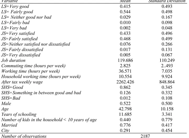
The resulting sample consists of 2187 observations for which descriptive statistics are presented in Table 1. Here we see that almost 96 percent of the individuals in the sample find their life to be very good or fairly good and some 90 percent are very satisfied or fairly satisfied with their job. So the distributions of these two subjectively derived variables are both rather skewed. We also see that the average job duration in the sample is almost 10 years (119 months). Individuals spend on average some 3 hours on commuting and about 36.5 hours working per week. The average hours spent on household work is around 10.5 hours. The average net weekly wage amounts to some 2262 SEK.
We also see from Table 1 that 86 percent find their health to be good. Slightly more than half of the sample is male and the average age is 43 years. The average individual has some 12 years of schooling and 0.4 younger kids in the household. Some 78 percent are married and 29 percent live in a city.
10
/Table 1 about here/
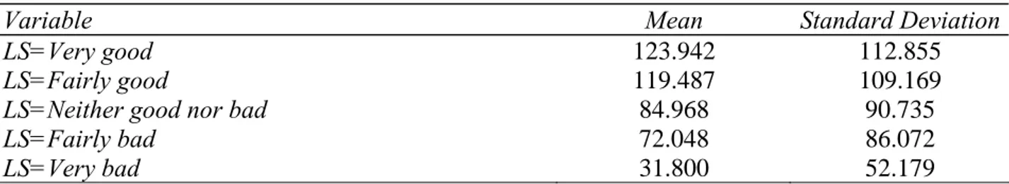
Table 2 outlines the relationship between the variables on life satisfaction and job duration. The relationship is strikingly monotonic. The more satisfied an individual is with life the longer has he/she been working in the current workplace (or ‘establishment’). Hence, there appears to be a relatively strong relationship between a choice variable like job duration that is supposedly correlated with the utility of an individual, and a variable on subjectively reported life satisfaction. Hence, even though many economists still may be sceptic about subjective assessments to measure an individual’s utility, it seems to correlate fairly well with observed choices which are usually taken as an accepted way to reveal preferences in main stream economics.
/Table 2 about here/
A similar picture pertains to the relationship between job satisfaction and job durations that tend to be longer the more satisfied an individual is with his/her job, although the relationship is not entirely monotone in this case. Thus, employment relations that are characterized by satisfied employees tend to survive longer than relations with non-satisfied employees. This is completely in line with Akerlof et al (1988) who argue that job satisfaction is negatively related to job switching.
/Table 3 about here/
4. Results
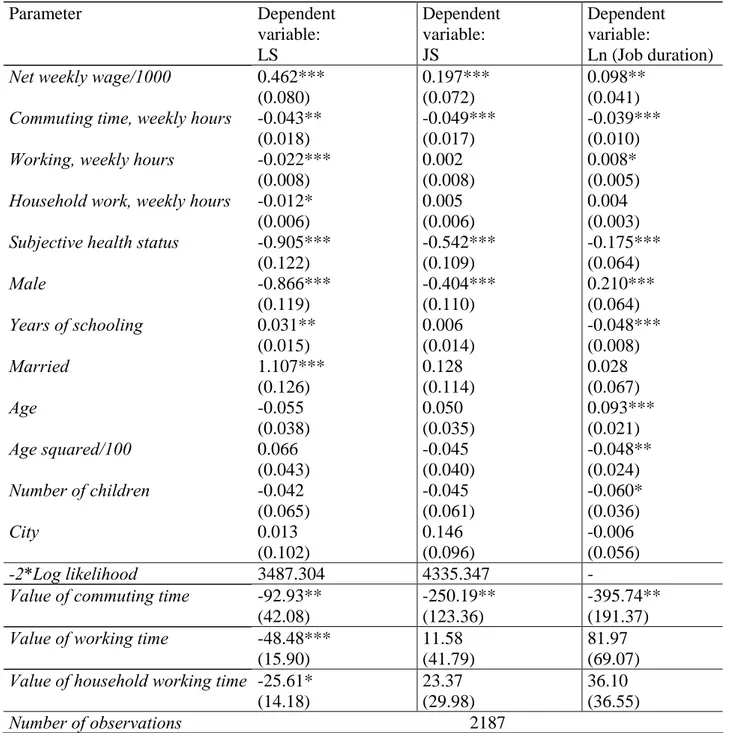
Table 4 presents the estimated models. Here we see that the effect of the net weekly wage on utility is positive according to all three models. Thus, the higher the wage, ceteris paribus, the higher is life satisfaction, job satisfaction and the longer is the job duration of the individual. Similarly, commuting time has a negative effect on the dependent variable in all three models, i.e. the longer the individual has to commute the less satisfied is he/she with his/her life and job, and the longer
the commute, the shorter is the duration of his/her job (The results of the job duration model are in line with those reported by Van Ommeren et al., 2000 and Isacsson and Swärdh, 2007).
However, working time has a significantly negative effect on life satisfaction but it has no significant effect on job satisfaction and job durations. One interpretation regarding the difference between the life satisfaction and job duration models is that an individual’s job offers are all constrained in terms of working hours, so the hours-restriction does not affect the duration of the current job. An alternative interpretation is, of course, that subjective assessments and revealed actions are different. Thus, although some aspect of life may reduce life satisfaction it is not certain that this leads to an action for improving the situation. We also note that time allocated to household work seems to affect life satisfaction in a negative way but it has neither an effect on job satisfaction nor on job durations, which may seem reasonable.
At the bottom of Table 4 we report the estimated values of time for each of the three dependent variables. First, we see that the value of commuting time is significantly different from zero at the five percent level of significance in all three models. It equals 93 SEK when the dependent variable is life satisfaction whereas it is more than twice as large, 250 SEK, when using job satisfaction as the dependent variable. The job duration model produces an even higher value, 396 SEK. Hence, all three estimates are well above the average net hourly wage rate which is about 62 SEK in the current sample and above the average gross hourly wage which is 84 SEK (these figures are not reported in Table 1).11 So the estimated values of time seem rather high considering the summary presented by Small (1992) who notes that a reasonable interval for the value of commuting time is around 20 to 100 percent of the gross hourly wage rate with a preferred estimate being some 50 percent of the gross hourly wage rate. But Isacsson and Swärdh (2007) also report a rather high estimate of the value of time in an empirical search model applied to a much larger sample of Swedish males. These ‘high’ estimated values may also be viewed in the light of the problem with hypothetical bias and studies showing that values of time tend to be higher in revealed preference studies than in stated preference studies (Brownstone and Small, 2005, and Isacsson, 2007).
Furthermore, another recent Swedish study that might support this argument is Vredin Johansson et al. (2006), who also estimate comparatively high values of commuting time from data on revealed preferences pertaining to mode choice.
/Table 4 about here/
We note, secondly, that the value of working time in the model of life satisfaction is surprisingly close to the average net hourly wage rate in the sample. Thus, according to the measures on life satisfaction, the average individual values changes in working time to be close to the net hourly wage rate which would correspond to the prediction in a conventional static labour supply model. The models based on job satisfaction and job durations indicate, however, no significant value of working time. Thirdly, according to the model based on life satisfaction, the average individual values household work to less than half of the average hourly net wage rate. The two other models indicate no willingness-to-pay for reducing time working in the household, which may be less surprising since these models are based on dependent variables related to the current job.
The effects of the control variables on the dependent variables exhibit some variation between the models. Subjective health status indicates that life satisfaction increases with the health of the individual. This is also the case with job satisfaction and job durations. Males seem to be less happy with their lives and less satisfied with their jobs than females but they tend to have longer job durations than women. Schooling increases life satisfaction but has no significant effect on job satisfaction and a negative effect on job durations. Married individuals tend to be more content with their lives than unmarried individuals. But marriage has no effect on job satisfaction or job durations. Age does neither affect life satisfaction nor job satisfaction but job durations are increasing on average, but at a diminishing rate, with the individual’s age. Number of young kids does neither raise life satisfaction nor job satisfaction but seem to decrease job durations. City dwellers are no more satisfied with their lives and jobs than people outside cities. In addition, the conditional mean for job durations do not differ between cities and outside cities.
11
As noted in section 2, a potential restriction of using the models in Table 4 to estimate the value of commuting time is the inclusion of hours of work and household working time as controls in the models. For this reason we re-estimated the models in Table 4 excluding working hours and household working time from the estimation equations. The results of this exercise are presented in Table 5. Although the differences compared to the models in Table 4 appear to be rather small, we note that the differences in the estimated value of commuting time are now somewhat smaller between the three models. More specifically, the estimated value of commuting time in the model of life satisfaction in Table 5 is around 113 SEK. It is some 251 SEK in the model of job satisfaction and some 304 SEK in the model based on job durations.
We also performed some sensitivity tests of the estimated models. These tests are not reported in any separate tables. Instead, they are discussed in the following. First, and as mentioned previously, we used an ordered probit rather than an ordered logit to estimate the models of life satisfaction and job satisfaction. But this did not alter the conclusions from the ordered logit model in any substantial way.
Secondly, we estimated a set of models where we included interactions between the commuting time and the city dummy variable, since commuting is likely to be more stressful in cities than outside of cities. The interacted variable was, however, not significantly different from zero at the 10 percent level of significance in any of the three models.
Finally, we included a set of dummy variables to control for working environment. These controls were based on information regarding stress, noise, physical and psychic demands, the degree to which the job is performed at a computer screen and whether the job involves repetitive work. The effect of including these controls was primarily to reduce the parameter for the net weekly wage in the three models, which tends to increase the estimated values of time. Inclusion of these variables also reduced the parameter for household work in the model of life satisfaction. An additional
effect was an increase of the standard errors of the estimated values of time in the three models. Hence, the value of household working time in the model of life satisfaction and the value of commuting time in the model of job satisfaction were insignificantly different from zero at the 10 percent level of significance when including controls for working environment. The value of commuting time in the models of life satisfaction and job durations was still significantly from zero at the 10 percent level of significance, however. Furthermore, the value of working time in the model of life satisfaction was significantly different from zero at the 5 percent level of significance even after adding the additional controls for working environment.
5. Conclusions and discussion
The most striking of our results is that although the estimated models are very different regarding the dependent variable used to measure the individual’s utility, they produce estimates of the value of commuting time that are all on the high side compared to previous estimates (cf. Small, 1992). In other words, no matter which variable we use to estimate the parameters of the utility model, they all do produce high estimates of the value of commuting time. In addition, the differences between the estimated values of commuting time were smaller when excluding working hours and household working time from the models. This might be good news for proponents of using subjective assessments to obtain policy relevant estimates of economic trade-offs, although the estimated value in the model based on job duration data was found to be higher than in the other two models.
In addition, the three models do not produce so similar results regarding the value of working time. We note, however, that the estimated value of working time from the life satisfaction model was rather close to the average net hourly wage rate in the sample, which is expected from a simple static model of labour supply. We also found that household working time affected life satisfaction but had no effects on job satisfaction and job durations. This may seem reasonable since household working time is not an attribute of the individual’s job. Both of these findings might suggest that data on life satisfaction are useful for estimating economic trade-offs. However, we did not find
that commuting had a larger negative effect on life satisfaction in cities than outside of cities. This seems counterintuitive, but may be the result of the rather small number of observations that identify the city-commuting time interaction.
Even though Kahneman et al. (2004) use data from the day reconstruction method (DRM) where individuals report the time allocated to different activities along with how they felt during each activity and we use data obtained from a global evaluation of life satisfaction (cf. Kahneman et al., 2006), we believe their results are useful for a final assessment of our results. They report that morning commutes are associated with the lowest ‘net affect’, or mood, among a large set of activities. They also find that individuals’ net affect is rather low when working and when commuting in the evening. Furthermore, household work seems to be associated with higher net affect than commuting and working. Hence, if general assessments of life satisfaction are related to more elaborate surveys like the DRM, it seems reasonable to find commuting to have a larger negative effect on life satisfaction than work and household work. This is consistent with the results of our model of life satisfaction. It may also seem reasonable to find working to have a stronger negative effect on life satisfaction than household work, which is also the case regarding the point estimates provided by our estimated model of life satisfaction. In sum, in spite of the caveats of using global evaluations of life satisfaction discussed by Kahneman et al. (2006), the estimated parameters of the various time related activities in our model of life satisfaction seem to be more or less in line with the results reported by Kahneman et al. (2004).
Acknowledgments
We are grateful for financial support from the Swedish National Road Administration and VINNOVA (the Swedish Governmental Agency for Innovation Systems). Seminar participants at the Swedish Institute for Social Research and at Dalarna University provided valuable comments on a previous draft of this manuscript. The usual disclaimer applies, of course.
References
Ahn, Namkee (2007), “Value of Intangible Job Characteristics in Workers’ Job and Life Satisfaction: How much are they worth?”, Documento de Trabajo 2007-10, Serie Nuevos consumidores, Cátedra Fedea-BBVA.
Akerlof, G.A., Rose, A.K. and Yellen, J.L. (1988), “Job Switching and Job Satisfaction in the U.S. Labor Market,” Brookings Papers on Economic Activity, Vol. 1988, No. 2, pp. 495-594.
Blanchflower, D.G. and Oswald, A.J. (2007), “Hypertension and Happiness across Nations”, Warwick Economic Research Papers No 792.
Booth, A. L. and van Ours, J.C. (2007), “Job Satisfaction and Family Happiness: The Part-time Work Puzzle”, IZA Discussion Paper No. 3020.
Brownstone, D. and Small, K. A. (2005), “Valuing time and reliability: assessing the evidence from road pricing demonstrations,” Transportation Research Part A, 39
Böckerman, P. and Ilmakunnas, P. (2006) “Do Job Disamenities Raise Wages or Ruin Job Satisfaction?”, International Journal of Manpower 27 (3), pp 290-302.
Chen, Y.Q. and Wang, Y. (2005), “Linear Regression of Censored Length-biased Lifetimes,” UW
Biostatistics Working Paper Series, Paper 258, The Berkeley Electronic Press.
Clark, A.E. (1997), “Job Satisfaction and Gender: Why are Women So Happy at Work?”, Labour
Economics, 4, pp. 341-372.
Devine, T. J. and Kiefer, N. M. (1991), Empirical Labor Economics - The Search Approach, New York: Oxford University Press.
Erikson, R. and Åberg, R. (1987), Welfare in Transition - Living Conditions in Sweden 1968-1981, Oxford: Clarendon Press.
Flinn, C.J. (1986), “Econometric Analysis of CPS-Type Unemployment Data,” Journal of Human
Resources XXI 4, pp. 456-484.
Frey, B.S., Luechinger, S. and Stutzer, A. (2004), “Valuing Public Goods: The Life Satisfaction Approach”, Center for Research in Economics, Management and the Arts, Working Paper No. 2004-11.
Frey, B.S. and Stutzer, A. (2002), “What can Economists Learn from Happiness Research?”,
Fritzell, J. and Lundberg, O. (1994), “Income distribution, Income Change and Health: On the Importance of Absolute and Relative Income for Health Status in Sweden”, World Health Organization Regional Publications - European Serie 54, 37-58.
Gronberg, T. J. and Reed, W. R. (1994), “Estimating Workers Marginal Willingness to Pay for Job Attributes Using Duration Data”, The Journal of Human Resources XXIX (3), 911-931.
Hensher, D. A. and Brewer, A.M. (2001), Transport: An economics and management perspective, Oxford: Oxford University Press.
Hwang, H, Mortensen D. T. & Reed (1998) W. R., “Hedonic Wages and Labor Market Search”,
Journal of Labor Economics, Vol. 16, No. 4, pp. 815-847.
Isacsson, G. (2007), “The trade off between time and money: Is there a difference between real and hypothetical choices?”, Swopec working paper, VTI series 2007:3.
Isacsson, G. and Swärdh, J-E. (2007), “An Empirical on-the-job Search Model with Preferences for Relative Earnings: How High is the Value of Commuting Time?”. Swopec working paper, VTI series 2007:12.
Kahneman, D., Krueger, A.B., Schkade D., Schwarz, N. and Stone, A. (2004), “Toward national well-being accounts”. American Economic Review, 94 (2), pp. 429-434.
Kahneman, D., Krueger, A.B., Schkade D., Schwarz, N. and Stone, A. (2006), “Would You Be Happier If You Were Richer? A Focusing Illusion”. Science, 312 (5782), pp. 1908-1910.
Keiding, N, Fine, J.P., Carstensen, L. and Slama, R. (2005), “Accelerated Failure Time Regression for Backward Recurrence Times and Current Durations,” Mimeo.
Lancaster, T. (1990), The Econometric Analysis of Transition Data, Cambridge University Press. Layard, R. (2005), “Happiness: Lessons From a New Science”, New York and London: Penguin. Rosen, S. (1986), “The Theory of Equalizing Differences”. in Handbook of Labor Economics, Editors O. Ashenfelter and R. Layard, Elsevier Science Publishers.
Small, K. A., (1992), Urban transportation economics, Harwood Academic Publishers: Philadelphia, Pennsylvania
Stutzer, A. and Frey, B.S. (2004), “Stress That Doen’t Pay: The Commuting Paradox”, IZA Discussion Paper No. 1278.
Van Ommeren, J., van den Berg, G. J., and Gorter, C. (2000), “Estimating the Marginal Willingness to Pay for Commuting” Journal of Regional Science 40(3), 541-563.
Van Praag, B.M.S. and Baarsma, B.E. (2005), “Using happiness surveys to value intangibles: The case of airport noise”. Economic Journal, 115 (500), pp. 224-246.
Vredin Johansson, M, Heldt, T. and Johansson, P. (2006), “The Effects of Attitudes and Personality Traits on Mode Choice,” Transportation Research Part A 40, pp. 507-525.
Yamaguchi, K. (2003), “Accelerated Failure-Time Mover-Stayer Regression Models for the Analysis of Last-Episode Data”, Sociological Methodology 33(1) pp. 81-110.
Table 1. Descriptive Statistics
Variable Mean Standard Deviation
LS=Very good 0.415 0.493
LS= Fairly good 0.544 0.498
LS= Neither good nor bad 0.029 0.167
LS=Fairly bad 0.010 0.098
LS=Very bad 0.002 0.048
JS=Very satisfied 0.433 0.496
JS=Fairly satisfied 0.468 0.499
JS=Neither satisfied nor dissatisfied 0.076 0.266
JS=Fairly dissatisfied 0.017 0.131
JS=Very dissatisfied 0.005 0.067
Job duration 119.686 110.249
Commuting time (hours per week) 2.825 2..493
Working time (hours per week) 36.571 7.035
Household working time (hours per week) 10.554 9.924
After tax weekly wage 2262.426 848.864
SHS=Good 0.862 0.345
SHS=Something in between good and bad 0.126 0.332
SHS=Bad 0.012 0.108
Male 0.522 0.500
Age 42.798 10.158
Years of schooling 11.685 3.341
Number of kids in the household < 10 years of age 0.440 0.779
Married 0.776 0.417
City 0.291 0.454
Number of observations 2187
Table 2. Job duration by level of life satisfaction
Variable Mean Standard Deviation
LS=Very good 123.942 112.855
LS=Fairly good 119.487 109.169
LS=Neither good nor bad 84.968 90.735
LS=Fairly bad 72.048 86.072
LS=Very bad 31.800 52.179
Table 3. Job duration by level of job satisfaction
Variable Mean Standard Deviation
JS=Very satisfied 116.476 111.167
JS=Fairly satisfied 128.230 111.012
JS=Neither satisfied nor dissatisfied 98.275 101.144
JS=Fairly dissatisfied 80.895 84.363
Table 4. Estimated models Parameter Dependent variable: LS Dependent variable: JS Dependent variable: Ln (Job duration)
Net weekly wage/1000 0.462*** (0.080)
0.197*** (0.072)
0.098** (0.041)
Commuting time, weekly hours -0.043**
(0.018)
-0.049*** (0.017)
-0.039*** (0.010)
Working, weekly hours -0.022*** (0.008)
0.002 (0.008)
0.008* (0.005)
Household work, weekly hours -0.012* (0.006)
0.005 (0.006)
0.004 (0.003)
Subjective health status -0.905*** (0.122) -0.542*** (0.109) -0.175*** (0.064) Male -0.866*** (0.119) -0.404*** (0.110) 0.210*** (0.064) Years of schooling 0.031** (0.015) 0.006 (0.014) -0.048*** (0.008) Married 1.107*** (0.126) 0.128 (0.114) 0.028 (0.067) Age -0.055 (0.038) 0.050 (0.035) 0.093*** (0.021) Age squared/100 0.066 (0.043) -0.045 (0.040) -0.048** (0.024) Number of children -0.042 (0.065) -0.045 (0.061) -0.060* (0.036) City 0.013 (0.102) 0.146 (0.096) -0.006 (0.056) -2*Log likelihood 3487.304 4335.347 -
Value of commuting time -92.93** (42.08)
-250.19** (123.36)
-395.74** (191.37)
Value of working time -48.48*** (15.90)
11.58 (41.79)
81.97 (69.07)
Value of household working time -25.61*
(14.18) 23.37 (29.98) 36.10 (36.55) Number of observations 2187
Notes: Standard errors in parentheses. The life satisfaction and job satisfaction models also include 4 alternative specific constants (intercept terms) and the job duration model includes an intercept. * denotes significantly different from zero at the 10 percent level, ** denotes significantly different from zero at the 5 percent level, and *** denotes significantly different from zero at the 1 percent level of significance.
Table 5. Estimated models, excluding working hours and household working hours Parameter Dependent variable: LS Dependent variable: JS Dependent variable: Ln (Job duration)
Net weekly wage/1000 0.381*** (0.069)
0.119*** (0.063)
0.133*** (0.036)
Commuting time, weekly hours -0.043**
(0.018)
-0.050*** (0.017)
-0.039*** (0.010)
Subjective health status -0.910*** (0.122) -0.541*** (0.109) -0.173*** (0.064) Male -0.807*** (0.104) -0.442*** (0.097) 0.197*** (0.056) Years of schooling 0.034** (0.015) 0.005 (0.014) -0.049*** (0.008) Married 1.046*** (0.117) 0.159 (0.106) 0.043 (0.062) Age -0.068* (0.037) 0.054 (0.035) 0.098*** (0.020) Age squared/100 0.083* (0.043) -0.050 (0.040) -0.053** (0.023) Number of children -0.044 (0.064) -0.039 (0.060) -0.060* (0.035) City 0.015 (0.102) 0.146 (0.096) -0.006 (0.056) -2*Log likelihood 3496.570 4335.997 -
Value of commuting time -113.062** (50.30) -250.92** (111.91) -303.58*** (112.09) Number of observations 2187
Notes: Standard errors in parentheses. The life satisfaction and job satisfaction models also include 4 alternative specific constants (intercept terms) and the job duration model includes an intercept. * denotes significantly different from zero at the 10 percent level, ** denotes significantly different from zero at the 5 percent level, and *** denotes significantly different from zero at the 1 percent level of significance.