Sports arenas in Sweden:
An economic analysis
A study investigating the impact of sports arenas on net migration and amenity
premiums.
MASTER THESIS WITHIN: Economics NUMBER OF CREDITS: 30 credits
PROGRAMME OF STUDY: Urban, Regional & International Economics AUTHOR: Andrew Gambina
Master Thesis in Economics
Title: Sports arenas in Sweden: An economic analysis Authors: Andrew Gambina
Tutor: Charlotta Mellander Date: 2018 – 05 – 21
Key terms: sports arenas, net migration, amenity premiums, Swedish, municipalities, fixed effects, feasible generalised linear squares
Abstract
This paper examines the impact of the building or renovation of a sports arena on net migration and amenity premiums. Swedish municipal data is collected for 289 municipalities over the period 1999 to 2016. The econometric analysis makes use of fixed effects (FE) and feasible generalised linear squares (FGLS) estimation techniques. This study builds on the growing literature of the intangible benefits of sports arenas and is one of the few Swedish studies of its kind. The results show that a sports arena built in year t, realises a 3.458% increase in net migration in year t + 5, for those sports arenas being used by football and ice hockey teams in the highest and second highest leagues.
Table of Contents
1. Introduction ... 1
Purpose ... 3
Limitations ... 3
2. Literature Review ... 4
Sports arenas as urban catalysts ... 4
Migration studies ... 6
2.2.1 Amenity led migration ... 6
2.2.2 Swedish studies on migration ... 8
3. Hypotheses ... 10
4. Data, Expected Relationships, Empirical Strategy and Model ... 11
Data ... 11 4.1.1 Dependent Variables ... 12 4.1.2 Independent Variables ... 12 4.1.3 Control Variables ... 12 4.1.4 Expected Relationships ... 15 Empirical Strategy ... 15 Empirical Models ... 17 5. Results ... 17 Descriptive Statistics ... 17 Correlation Analysis ... 21 Regression Analysis ... 22 6. Robustness Diagnostics ... 28 7. Analysis of Results... 26 8. Conclusions ... 29 9. References ... 30 10. Appendix ... 37 Appendix A ... 37 Appendix B ... 39 Appendix C ... 40 Appendix D ... 46 Appendix E ... 48
1
1. Introduction
Between 2004 and 2010, 30 arenas, used for sport, culture, and event purposes, were planned to be built across various municipalities in Sweden (SOU 2007:32:187), and since then more arena building projects have been added and completed, not least the 50,000 seating capacity ‘Friends Arena’ in Solna. Sports arenas are funded by several organisations in Sweden, such as municipalities, private companies, and sports associations. Municipalities tend to be heavily involved in both the building and financing process of sports arenas, which often means that taxpayer money is going towards sports arena investment rather than healthcare, education, or transport improvement (Suneson, 2018). But why are municipalities stepping in to fund sports arenas in the first place?
Municipalities are funding sport arenas for two main reasons: (1) Sports arenas are expensive to build and operate, meaning that sports clubs or private investors alone rarely reap enough revenues to cover the costs of construction and operation (Siegfried and Zimbalist, 2000). (2) Municipalities see investment in sports arenas as being important in enhancing and preserving long-term social and cultural activities within the municipality (Jasarovic, 2018; Sandvikens kommun, 2017). Municipalities, therefore, end up either building and owning the sports arena themselves (Kägo, 2014; Bjurner, 2014) or co-financing sports arenas with other investors (Ivarsson, 2015).
Regulations implemented by Swedish football and ice hockey associations on sports arena requirements are causing a great deal of debate within the local media on sports arenas in general and who should be financing them. In a survey done by Sveriges Radio, Sweden’s national publicly-funded radio and news broadcaster, they asked municipality leaders what they think of sports arenas and the requirements demanded by sports federations for elite teams. Out of the seven municipality representatives that answered, six said that they are worried about these demands. Municipality representatives are worried because sports arena standard demands are creating costs for sports teams that they cannot afford. This, in turn, puts pressure on municipalities to find a solution to the sports teams’ financial problems through financial help. Most municipalities are already in financial difficulties with other commitments, therefore subsidizing sports arenas,
2
which rarely make profits, could put the municipality into further financial problems (Sandberg and Lindström, 2011).
The public debate on sports arena funding is not just happening here in Sweden, in the US, for example, sports arena funding is also a highly debated topic. Dorfman (2015), writing in Forbes magazine, claims that the tax revenue collected from sports arenas does not outweigh the cost of public financing. The reason for this, he continues, is because most sports arenas do not attract enough people from outside of the city. Furthermore, in another US media publication, Anzilotti (2016) writing in Citylab claims that “an estimated $12 billion in public money has been used to finance stadiums over the past 15 years, and the Brookings report places the federal tax revenue loss resulting from these projects at $3.7 billion” (Anzilotti, 2016, paragraph 3).
So, if sports arenas do not generate enough tax revenue to cover its costs, how do governments or municipalities justify large sum investments in them? Governmental entities rationalize sports arena investments through economic impact studies. These studies are commonly carried out by consultants or large consulting firms, which attempt to forecast the economic benefits by estimating spending multipliers which typically conclude that investing in arenas will result in large economic benefits. The economic benefits referred to in these studies are additional sums of tax revenue, income, and new job creation (Zimbalist and Noll, 1997). Has this been the case in practice? Past literature has focused on the employment and income effects of sports arena construction (Coates and Humphreys, 2002; Baade, 1996; Baade and Dye, 1990) and the consensus amongst these studies is that there is little or no support for the claim of a positive correlation between sports teams or arenas on job creation and incomes. In addition, researchers studying sports arenas have claimed that “a new sports facility has an extremely small (perhaps even negative) effect on overall economic activity and employment” (Zimbalist and Noll, 1997, paragraph 7).
Then why do sports arenas continue to be built if they aren’t increasing employment and income levels? Professional sports events such as a game of football between two neighbouring cities give people something to talk about and provide opportunities for people of different backgrounds to come together. In doing so, this may result in a greater sense of community, civic pride and consumption benefits to those attending games
3
(Coates and Humphreys, 2003). Furthermore, sports arenas are amenities that have the potential to attract people towards the area where the arena is located and act as urban catalysts (Rosentraub and Cantor 2012; Chapin, 2004).
Amenities are known to be an important factor when one is deciding where to reside and has led to people moving location in search for better city attractions (Fasshauer and Rehdanz, 2015; Clark et al., 2002; Knapp & Graves; 1984). This attraction factor that sports arenas possess will be the focus of this paper. Net migration levels for both municipalities with and without sports arenas are studied. Studies of this kind have not been many, with Värja (2014) being the only author to do so. In the author’s paper, she analyses whether a municipality’s net inbound migration and per capita income are affected when a local football or ice hockey sports team enters or exits the highest or second highest national leagues in Sweden. This paper follows a similar path when it comes to analysing net migration in Sweden, however, focuses on sports arenas rather than sports teams. Moreover, this paper introduces the concept of amenity premiums in a sport arena study, which can be understood as the higher rents paid when taking into account wages. The greater the difference between rents and wages in a municipality, the greater is the amenity premium and therefore the desire to live in the municipality, which is an concept borne out from Glaeser et al.’s (2001) spatial equilibrium equation1.
Purpose
This paper analyses sports arenas in Sweden to find out whether a relationship exists between municipalities with sports arenas and net migration. Furthermore, this paper investigates whether municipalities with sports arenas have positive amenity premiums, which could be also viewed as municipality attractiveness in terms of incomes and housing prices.
Limitations
The economic software used, Eviews 10, is a limitation when considering the spatial data that is collected for this study. Tests such as Moran’s I or Mantel, which measure spatial autocorrelation in a model are not available in the software program. Furthermore, Eviews 10 provides restricted estimation options when spatial dependence is present. Another
4
limitation of this study is the availability of data for some independent variables. Data for some variables are not available for the full time period analysed (1999 to 2016) and therefore creates an unbalanced panel which leads to fewer observations when running regressions. Lastly, the multiple sources needed to collect information on sports arenas means that the data is more subject to measurement error.
2. Literature Review
A common justification for subsidizing sports arenas is that sports arenas lead to positive outcomes that citizens can enjoy by, for example, attending their local football team matches or through civic pride knowing that your favourite team is doing well. Since these benefits are not traded in the market and aren’t given a price, calculating them has been seen to be problematic (Coates and Humphreys; 2003). In this paper, a look at the studies that have highlighted the intangible benefits of sports arenas will be taken. The intangible benefits of sports arenas have been studied in the literature following three main themes:
(1) Sports led urban (re)development studies, that analyse what a certain sports event such as the Commonwealth games or more specifically, what the building of a sports arena has done in terms of economic development for the city or region.
(2) Hedonic price model studies, that try to capture the externalities arising from the construction of sports arenas on housing price values.
(3) Contingent valuation approach studies, that usually use surveys to collect data on the willingness to pay (WTP) for a new sports arena within the area.
A further look at the literature will be taken for sports led urban (re)development studies due to its relevance with the purpose of this study.
Sports arenas as urban catalysts
Studies in sports-led urban (re)development literature often take a descriptive style with little or no empirical work. There is a prevalent focus amongst these studies on the architecture and iconic stature of new sports arenas (Maenning & Plessis, 2009; Ahlfeldt & Maenning, 2010). These authors claim that architectural attributes play an important part in the success of sports arenas. A vast majority of studies in this field do not conclude
5
on whether sports arenas create urban redevelopment benefits large enough to justify sports arena cost. The reason for this is because the benefits of such sports arenas are hard to measure whilst the costs are not.
In a study by Austrian and Rosentraub (2002), the authors examine the implementation of sports policies in four cities, more specifically whether the vitality or centrality of a downtown area was enhanced or sustained by the introduction of a sports arena. They find positive evidence that the focus on the sports and hospitality sector did refocus some level of development activity into the downtown areas of two cities. Furthermore, sports arenas managed to create an excitement about downtown areas which created more jobs in suburban locations. In another study, Ahlfeldt and Maennig (2010), discuss the transition in international arena architecture and review the first empirical evidence of the impact of an arena at the neighbourhood scale. The results show that newly constructed arenas can be a good means of carrying out city development policies at small-scale levels. The authors conclude that at the city level, the primary aim should be an increased influx of mass tourism generated by iconic sporting arenas. Trendafilova et al. (2012), investigate the role that sport played in revitalizing Detroit, Michigan. The authors carry out interviews with an expert panel of economic development stakeholders and find that sport activities are successful when used as a tool to enhance the downtown image of Detroit by creating opportunities for entertainment.
In another US study, Cantor and Rosentraub (2012), examine the effects of the building of a new ballpark on neighbourhood economic development in San Diego. They find an increase in the number of higher income households, a larger proportion of residents fifty years and older eight years after the ballpark was constructed, an increase in the proportion of individuals who are employed in sectors associated with high education levels, and relatively stable house prices shortly after the economic downturn in 2008. The authors conclude that the ballpark district should be considered a success. Buckman and Mack (2012) study two arena development projects in Denver and Phoenix with a focus on the role of urban form the arenas are built around. A figure-ground analysis is utilised five years prior and post arena construction to show the increase or decrease in density for both projects. The authors claim that the goals for both arena construction projects were to revitalize their respective downtown areas by attracting both businesses
6
and residents to the area. However, despite the similar socio-economic and demographic characteristics of both projects, the Denver arena project was more successful, with a bustling hub of shops, restaurants and apartment complexes. The authors conclude that the Denver arena is proof that arenas can have a positive impact on downtown communities when an arena is built in the right context.
In more recent studies, Crompton (2014) analyses the returns on investment in sports arenas from proximate structural development. The author finds that associate developments around an arena are critical ingredients at city level whilst at regional level businesses that feed off sports arenas are vital. Lastly, the author concludes that investments in sports arenas will only be effective if they are part of an integrated coherent master plan involving all parties such as city mayors, local authorities, and sports arena investment owners.
The literature in this field of study produces encouraging results for sports arenas to be used as economic regenerators of downtown areas in cities. For these areas to become a success it involves people and businesses moving towards the area where the arena is being built (Buckman & Mack, 2012; Cantor & Rosentraub, 2012).
Migration studies 2.2.1 Amenity led migration
The definition of amenities is not academically agreed upon by authors within this field of study. Amenities have been described as “anything that shifts the household willingness to locate in a particular location….and includes weather, landscape, public services, public infrastructure, crime, ambience, and so on (e.g., Roback, 1982; Gyourko & Tracy, 1991; Dalenberg and Partridge, 1997; Glaeser, 2007)” (Partridge, 2010, page. 518). Whilst amenity migration has been described as “the movement of people based on the draw of natural and/or cultural amenities” (Abrams and Gosnell, 2009, page. 305) Studies in this field include several papers that are descriptive in nature and often debate which amenities should be included (Abrams and Gosnell, 2009; Storper and Scott, 2009; Greenwood 1985). There are many papers that either focus on cultural amenities (Glaeser et al., 2001; Clark et al., 2002) or natural amenities (Graves, 1980; Rappaport, 2006,
7
Daams and Veneri, 2017). Another clear divide in the literature are those studies that focus specifically on the relationship between amenities and migration (Fabhauer and Rehdenz, 2015; Rupasingha and Goetz, 2004; Knapp and Graves, 1989) and studies that focus on amenities and regional /city development (Glaeser et al. 2001; Florida et al. 2008; Gottlieb 1994).
One of the first studies to highlight the importance of local public goods, (Tiebout, 1956) discusses the Musgrave-Samuelson analysis which formulates ideas on the efficient provision of public goods. The author makes use of this analysis to formulate his own model and come up with a solution for the level of expenditure for local public goods. In another well-cited paper, Roback (1982) discusses the role of wages and rents in allocating workers to locations with various quantities of amenities. The author develops his own theory and argues that the value of an amenity is reflected in both the wage and rent gradients. Furthermore, Roback remarks that the decomposition depends on the influence of the amenity and consumer preferences.
In a US study, Clark and Hunter (1992) integrate economic opportunities, amenities and state and local fiscal factors in determining migration using a life-cycle framework. The authors conclude that amenities, as well as labour market opportunities, are important determinants of migration. Furthermore, they find that amenities are consistently found to influence middle and older aged males to a greater extent than younger males. In an influential paper, Glaeser et al. (2001) claim that the demand for cities stems from the desire to reduce transportation costs for goods, people and ideas. Furthermore, they introduce a spatial equilibrium equation where; urban productivity premium + urban amenity premium = urban rent premium. This equation explains how wages (urban productivity premium) and the quality of life in a city (urban amenity premium) are offset by housing rents (urban rent premium) for the same city. Moreover, this equation implies that amenity premiums for municipalities may be measured by taking the difference between the rent premiums and wage premiums.
In a descriptive study undertaken by Clark et al. (2002), the authors highlight the critical role and political choices of amenities in relation to urban growth dynamics. They conclude that the decision of where to live and enjoy life can play as large if not larger
8
role than job opportunities when deciding on where to locate. In a European study, Buch et al. (2013) investigate the determinants of the migration balance of German cities between 2000 and 2007 with a focus on the mobility of workers. They consider 71 German cities with a population of at least 100,000 inhabitants and find that both local labour market conditions and amenities matter for the residential choice of workers. 2.2.2 Swedish studies on migration
Värja (2014) analyses the success of football and ice hockey teams on net migration and per capita income growth. The reason why the author looks at football and ice hockey teams and not other teams from other sports is due to, she claims, that these two sports have the highest spectator attendance during matches. The author uses a dummy variable to indicate whether a football or ice hockey team is in the highest or second-highest league. Her benchmark model assumes that the explanatory variables effect net migration, the dependent variable, five years later. The author finds no positive correlation between the rate of local average income growth and successful sports teams. Moreover, results for the net migration rate are insignificant when all municipalities are considered, however a small positive effect between ice hockey teams and net migration is found when the 3 major cities, Stockholm, Göteborg and Malmö are taken out from the analysis.
Lundberg (2003) studies the factors that determined municipal net migration and average income growth during the 1980s. The author does this by including:
(1) Economic “opportunity” variables such as the share of people with a university degree, the average income level and the unemployment rate.
(2) Local government policy decisions such as the local income tax rate, local government expenditures and local government investments.
(3) National government policy variables such as intergovernmental grants and university presence
(4) Socio-economic and demographic structure variables such as the share of the local industrial structure, population density, population aged 0 to 15 years, population aged 65 years or above, and a dummy variable indicating whether a municipality is located in the north.
(5) Political composition of local council such as the share of representatives from a particular party and a qualified political majority in the local council.
9
Lundberg finds that initial endowments of human capital have a highly significant positive effect on net migration and a negative relationship between the unemployment rate and net migration. Furthermore, the author highlights the importance of local policy decisions on net migration and claims that local public investments have had a positive subsequent effect of net migration rates.
Nelson and Wyzan (1989) examine the importance of several fiscal and traditional market variables on Swedish local private labour demand and interjurisdictional migration. Their results show, that on a regional level, taxes negatively affect both migration and labour demand, whilst on a municipality level results are negative but more ambiguous. They find destination wages to have a significantly positive impact on municipality level migration but no effect on the regional level. The authors conclude that the disparities between the municipality and the regional results suggest that there are benefits in examining migration at the lowest level of aggregation possible. In another study, Westerlund (1997) analyses the impact of aggregate labour turnover and regional labour market conditions on county net migration using a neoclassical flexible wage model and a fixed wage model. The author finds that regional differences in employment prospects seem to be the key factor when individuals decide where to migrate. In a regional study, Aronsson et al. (2001), analyse regional income and net migration growth rates between 1970 and 1995. The explanatory variables for both dependent variables, the migration rate and growth rate of income, are measured in five year intervals. They find that indicators of future possible earnings and the initial endowment of human capital are positively related to net migration.
In another study, Lundberg (2006) uses spatial econometrics to analyse the average income growth and net migration rate for Swedish municipalities for the years 1981 to 1999. A key finding in this study is the positive correlation found between net migration rates in neighbouring municipalities, which means that net migration tends to spillover to neighbouring municipalities. To tackle this issue, the author uses a spatial lag specification to account for spatial dependence in the net migration model. In a more recent study, Malmberg et al. (2011) examine household gains and losses from migration within the Swedish urban hierarchy. They focus on whether increases in disposable income outweigh changes in housing costs when moving up the urban hierarchy to larger
10
population-growth regions. The authors reveal that the urban hierarchy is important to consider when estimating migrant outcomes. They claim that migrants moving to larger labour markets add approximately double the amount to their nominal income when compared to migrants moving to smaller labour markets. The authors highlight the importance of taking regional housing cost disparities into account when estimating economic outcomes of domestic migration. Gärtner (2014) uses labour market, demographic, and geographic explanatory variables to explain internal county migration in Sweden from 1967 to 2003. The author uses a dynamic panel model and finds that: higher wages correlate with an increase in migration, whilst unemployment encourages people to leave to counties with increasing vacancies, and a higher share of younger people in a county attracts people to migrate to the same county.
3. Hypotheses
Based on the literature review and comprehensive data collection the following hypotheses are drawn:
Hypothesis 1: A sports arena built in municipality i at time t is positively related to net migration in year t + 5 for the same municipality.
Hypothesis 2: A sports arena renovated in municipality i at time t is positively related to net migration in year t + 2 for the same municipality.
Hypothesis 3: Municipalities that have a sports arena built realise positive amenity premiums five years later.
Hypothesis 4: Municipalities that have a sports arena renovated realise positive amenity premiums two years later.
The impact of a sports arena renovated is examined in this paper even though studies on this have been few. Baade (1990) can be given as an example of an author who has investigated sports arenas renovated. The reason this paper investigates sports arenas renovated is mainly due to the Swedish setting, where sports teams entering the highest
11
and second highest divisions in their respective sport are usually required to renovate their sports arenas to meet the arena specification requirements set by the sport association. Furthermore, the time period for a sports arena to influence net migration might take a few years to be realised. It might take time for people to move from one place to another due to financial, family or work reasons. Both Aronsson et al. (2001) and Värja (2014) use a five year time period for their explanatory variables to influence net migration. Furthermore, Buckman and Mack (2012) look at demographic changes five years before and after stadium construction. Therefore, the impact of a sports arena built is examined five years after its construction. Since the renovation of a sports arena involves making adjustments to an existing building that has been used and known by individuals for a number of years, the effects of a sports arena renovation are likely to be realised sooner than a sports arena built. Therefore, a sports arena renovation is assumed to have an effect on net migration two years later.
Amenity premiums, which can be computed by taking the difference between rent premiums (the higher housing cost paid to live in certain areas) and wage premiums (the higher wages earned in certain areas), measures the quality of life of certain areas. This measure is introduced for the first time in a sports arena study. A sports arena, which is an amenity, may increase amenity premiums in the municipality were the arena was built, by making rent premiums increase, it is well documented in the literature that sports arenas increase housing prices in close proximity (Tu, 2005; Ahlfeldt and Maennig, 2008), and wage premiums remaining relatively unchanged.
4. Data, Expected Relationships, Empirical Strategy and
Model
Data
All primary data was gathered from Statistics Sweden (SCB). Annual panel data was collected for the period 1999 to 2016 for Sweden’s 289 municipalities. To avoid including municipalities that have changed borders during the time period analysed, all data related to Knivsta municipality was added back to Uppsala, which was where Knivsta was borne out of. The total observations obtained for a balanced panel is 5202.
12 4.1.1 Dependent Variables
Netmig
To calculate net migration, the internal in and out migrations per municipality is collected separately and later logged. Once logged, the internal in migrations is subtracted from the internal out migrations. Internal here refers to migrations happening within Sweden’s municipalities. Data availability for net migration is available from 1997 to 2017.
Amenitypremium
The amenity premium variable is measured by estimating an OLS regression of income per capita on average purchase house prices in thousand SEK. The unstandardized residuals from this regression represents the desire to live within a municipality, where higher amenity premiums reflect higher levels of willingness to live in the area.
4.1.2 Independent Variables Arenas_built
This is a dummy variable that takes a value of 1 if a new football or ice hockey sports arena is built, for both football and ice hockey teams that are in the highest or second highest division, with post-construction periods also having a value of 1. A value of 0 is given if no new sports arena is built for the same selection of arenas during the time period analysed.
Arenas_ren
This is another dummy variable that takes a value of 1 if a football or ice hockey sports arena is renovated and a value of 0 if no football or ice hockey arena is renovated for both football and ice hockey teams in the highest and second highest division season for the period 1999 to 2016.
4.1.3 Control Variables
Economic “opportunity” variables
Degree_pc
The share of people with a post-secondary education that lasts three years or more is collected as a proxy for human capital within a municipality. Individual high levels of human capital means that a person has spent time and effort in investing in oneself. Therefore a person with a post-secondary education of at least three years is believed to
13
have put in this investment. People with high levels of human capital want to be in municipalities where there are other people with high levels of human capital and thus municipalities that have an initial high level of human capital are attractive to these kind of individuals. Lundberg (2003) uses a similar measure to proxy human capital by measuring the percentage of inhabitants with a university degree and finds a positive relationship between endowments of human capital and net migration. The variable is divided by the total population to obtain per capita measures. Data is available from 1985 to 2017.
Avg_income
Avg_income represents the municipal average earned income for residents sixteen and above in SEK. Municipalities with high average income levels are attractive for an individual who is deciding on where to locate. Lundberg (2003) uses a similar measurement for the average income variable in his net migration model but calculates the average earned income for residents aged twenty and above. Lundberg (2003) assumes a positive relationship between average income and net migration however results show a negative relationship instead. Data available is from the year 1991 to 2016.
Employed_pc
The share of people sixteen and above that are gainfully employed is used as a proxy of employment within a municipality. The more people employed in a municipality the stronger is the labour market in that municipality and thus the more attractive is that municipality to individuals migrating for better work opportunities which from the literature review is seen to be a key reason as to why people migrate. Lundberg (2003) and Gärtner (2014) use the unemployment rate as a variable in their net migration model and find a negative correlation between net migration and unemployment. The variable is divided by the total population to obtain per capita measures. Data available is from the year 2001 to 2016.
Local government policy variables
Taxrate
The local percentage tax rate is collected to give an understanding of the varying tax rates per municipality. High taxes in a municipality can disincentivise people to move into the
14
municipality. Lundberg (2003) uses a similar variable in his net migration model however includes the regional income tax rates in his measure. The author finds a negative relationship between the local income tax rate and net migration in his study. Data is available from 2000 to 2018.
National policy variables
Grants_pc
The Grants variable is collected from the income statement for municipalities by region provided by Statistics Sweden in SEK per capita for current prices. The variable in Swedish is referred to as “utjämningssystem” where poorer municipalities are given support by richer ones. Municipalities that receive high levels of grants are poorer to other municipalities and thus might not be an attractive location for potential migrants. Lundberg (2003) uses the same measure in his study and finds a small and positive relationship between grants and net migration. Data is available from 1998 to 2017.
Socio-economic and demographic variables
Families_pc
The share of families with children and young persons aged zero to twenty-one is collected per municipality and is a proxy. The higher the share of families with children in a municipality the more life and potential the municipality possesses. The variable is divided by the total population to obtain per capita measures. Data is available from the year 2000 to 2014.
Pop65_pc
Pop65 represents the share of people sixty-five years and above. This is a proxy for the share of the population that is retired. The more people sixty-five and above residing in a municipality the less attractive it is for potential migrants to move into the municipality since migrants, who are typically relatively young in age, would want to be in a municipality where there are individuals of approximately the same age. Lundberg (2003) measures the same variable in his study, however his regression models give opposing results for the relationship between the share of the population aged sixty-five and above and net migration. The variable is divided by the total population to obtain per capita measures. Data is available from 1968 to 2017.
15 Popden
Population density per square kilometer represents the popden variable. The closer people are to one another the easier it is to acquire information and knowledge thus making highly dense locations attractive places to live in. Lundberg (2003) uses the same measurement to account for population density in his net migration model. The author finds opposing results in the two models estimated in his net migration benchmark model. Data is available from 1991 to 2017.
4.1.4 Expected Relationships
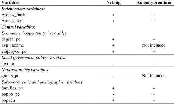
After presenting the dependent and independent variables and going through previous studies, the expected relationship signs for the variables included in the models are presented. Since amenity premiums and net migration are both measures of attractiveness, the same control variables are used except for avg_income, which is taken into account when estimating the amenitypremium measure, and grants_pc, which is assumed to have no effect on municipality attractiveness.
Table 1: Expected relationships between dependent, independent and control variables.
Variable Netmig Amenitypremium
Independent variables:
Arenas_built + +
Arenas_ren + +
Control variables:
Ecomomic ”opportunity” variables
degree_pc + +
avg_income + Not included
employed_pc + +
Local government policy variables
taxrate - -
National policy variables
grants_pc - Not included
Socio-economic and demographic variables
families_pc + + pop65_pc popden - + - + Note: _pc means that variables are in per capita form.
Empirical Strategy
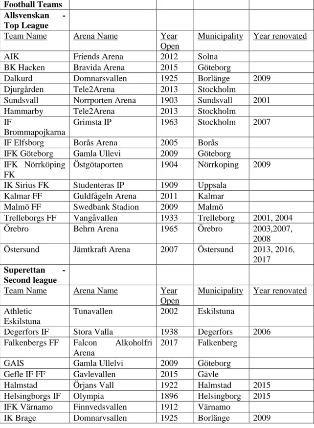
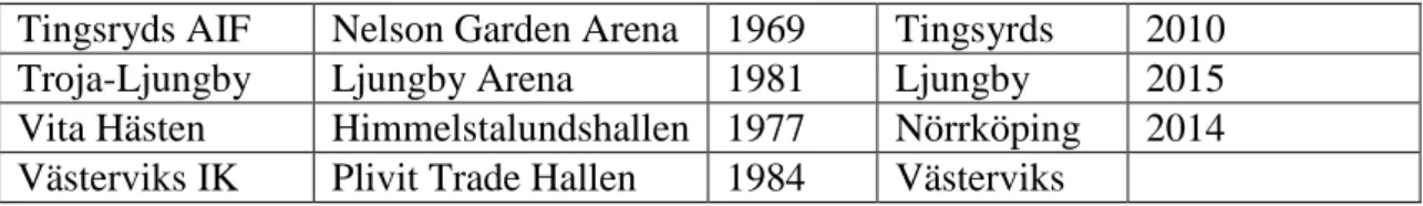
The sports arenas analysed are for those teams that are in the highest or second highest division in football and ice hockey for the season 2017/2018, where a clear list of all
16
sports arenas analysed may be seen in appendix A. Due to the time assumptions made for sports arenas built and renovated to influence net migration and amenity premiums the sports arena presence dummy variables are labelled arenas_built05 and arenas_ren02 reflecting the time periods it takes to impact net migration.
Variables degree, employed, families, and pop65 are divided by total population to obtain per capita measures. In addition, all variables except grants, and sports arena presence dummy variables are logged transformed to linearize the data. The grants variable is not log transformed so that negative value data is not lost. Before any model is run, a Breitung unit root test is made to identify whether variables in the model are stationary (see appendix C, table 1). The advantage of using the Breitung unit root test over other unit root measures is that the Breitung unit root test includes individual fixed effects and individual linear trends as regressors. The results show that some variables are stationary at levels [I(0)] whilst others are stationary at first or second differences. This means that estimating a model using OLS could produce unreliable results. Granger and Newbold (1974) found that estimating an OLS regression for non-stationary data would likely result in misleading estimates of the parameters. This phenomenon is known as spurious regression analysis, where the OLS results show highly significant parameters even if there exists no economic relationship between dependent and independent variables.
Another test is made for serial autocorrelation by looking at the correlograms for all variables. The results show that all variables suffer from first-order correlation (see appendix C, tables 2 to 13). An AR(1) term is included in the regressions to account for this. In addition, a Hausman test is run, to check which model, a fixed or random effect model, would best fit the data. The Hausman test rejects the null hypothesis and shows that the fixed effects model would be the more suitable model to use (see appendix C, tables 14 and 15) and thus a fixed effect model is estimated. As a comparative model to the fixed effects model, a feasible generalised least squares (FGLS), which can produce unbiased estimators even when non-stationary variables are present (Baltagi et al., 2011), is estimated.
17 Empirical Models
For the empirical section of this paper, two main models are used. Model (1) aims to reveal the relationship between a sports arena built or renovated and net migration controlling for economic “opportunity” variables, local government policy variables, national policy variables and socio-economic and demographic variables, thus testing hypothesis 1 and 2. Model (2) tests hypothesis 3 and 4, by using a restricted set of control variables to illustrate the relationship between municipality attractiveness (amenitypremium) and sports arenas built or renovated.
𝑙𝑛𝑛𝑒𝑡𝑚𝑖𝑔𝑖𝑡 = 𝛼𝑖𝑡+ 𝛽𝑖(𝑎𝑟𝑒𝑛𝑎𝑠_𝑏𝑢𝑖𝑙𝑡)𝑡−5+ 𝛾𝑖𝑙𝑛(𝑒𝑐𝑜𝑛𝑜𝑚𝑖𝑐)𝑡 + 𝛿𝑖𝑙𝑛(𝑙𝑜𝑐𝑎𝑙 𝑔𝑜𝑣𝑒𝑟𝑛𝑚𝑒𝑛𝑡 𝑝𝑜𝑙𝑖𝑐𝑦)𝑡+
𝜑𝑖(𝑛𝑎𝑡𝑖𝑜𝑛𝑎𝑙 𝑝𝑜𝑙𝑖𝑐𝑦)𝑡+ 𝜔𝑖𝑙𝑛(𝑠𝑜𝑐𝑖𝑜 − 𝑒𝑐𝑜𝑛𝑜𝑚𝑖𝑐 & 𝑑𝑒𝑚𝑜𝑔𝑟𝑎𝑝ℎ𝑖𝑐)𝑡+ 𝐴𝑅(1) + 𝜀𝑖 (1)
𝑎𝑚𝑒𝑛𝑖𝑡𝑦𝑝𝑟𝑒𝑚𝑖𝑢𝑚𝑖𝑡 = 𝛼𝑖𝑡+ 𝛽𝑖(𝑎𝑟𝑒𝑛𝑎𝑠_𝑏𝑢𝑖𝑙𝑡)𝑡−5+ 𝛾𝑖𝑙𝑛(𝑒𝑐𝑜𝑛𝑜𝑚𝑖𝑐)𝑡+
𝛿𝑖𝑙𝑛(𝑙𝑜𝑐𝑎𝑙 𝑔𝑜𝑣𝑒𝑟𝑛𝑚𝑒𝑛𝑡 𝑝𝑜𝑙𝑖𝑐𝑦)𝑡+ 𝜔𝑖𝑙𝑛(𝑠𝑜𝑐𝑖𝑜 − 𝑒𝑐𝑜𝑛𝑜𝑚𝑖𝑐 & 𝑑𝑒𝑚𝑜𝑔𝑟𝑎𝑝ℎ𝑖𝑐)𝑡+ 𝐴𝑅(1) + 𝜖𝑖
(2) i represents each municipality and t represents each year. Ln denotes those variables that are logged transformed. Renovated sports arenas, (arenas_ren)t-2, replace βi separately in
both models.
5. Results
Descriptive Statistics
Descriptive statistics are presented for the variables used in models 1 and 2 in level form, except for grants_pc where data has been collected from the source as a per capita measure, for municipalities with and without sports arenas as defined in arenas_built. In Table 2 and 3, all variables except tax rate have a higher mean in municipalities with sports arenas. In addition, both netmig and amenitypremium have significantly greater means for municipalities with arenas which are encouraging signs for the hypotheses formulated. The difference between mean and median, maximum and minimum is large and is the reason for the high standard deviations recorded. Taxrate is the only variable in both tables that records a relatively low standard deviation. Due to high standard deviations, the data set is believed to be heterogeneous, and this is another reason in support of log transforming the variables, which decreases skewness. A Jarque-Bera (JB) test is applied at a 5% level of acceptance and all variables follow a non-normal distribution as the null hypothesis of normality is rejected. Observations are recorded for
18
the variables individual samples, hence the reason why variables have different observations which are restricted to data availability.
Table 2 - Descriptive statistics for variables used in model 1 and 2 for municipalities with arenas (as defined in
arenas_built)
Variable Obs. Mean Median Maximum. Minimum Std. Deviation Pr.JB test Netmig 190 66.779 55.000 1873.000 -4000.000 483.510 0.000 Amenitypremium 190 501.255 262.063 6293.119 -1068.169 1109.993 0.000 Degree 190 21102.180 10589.500 236621.000 903.000 37182.290 0.000 Avg_income 190 235135.300 232600.000 338600.000 169900.000 30327.660 0.000 Employed 189 59927.920 41394.000 499995.000 6987.000 80816.500 0.000 Taxrate 190 0.320 0.323 0.339 0.292 0.011 0.000 Grants_pc 190 7301.705 7358.000 16272.000 -7282.000 3712.129 0.000 Families 154 11178.730 8201.500 84315.000 1377.000 12691.560 0.000 Pop65 190 21399.260 16087.000 136559.000 3151.000 22802.300 0.000 popden 190 402.526 75.350 4999.100 8.600 994.467 0.000
Note: All variables are in level form except for grants_pc, which is in per capita form. * rejection of null hypothesis, H0: series normally distributed for JB test.
Table 3 - Descriptive statistics for variables used in model 1 and 2 for municipalities without arenas (as defined
in arenas_built)
Variable Obs. Mean Median Maximum. Minimum Std. Deviation Pr.JB test
Netmig 5012 -2.531524 -27 4408 -3091 241.7138 0.000 Amenitypremium 4723 -20.16483 -33.97543 5488.267 -1883.209 784.4591 0.000 Degree 5012 3258.326 1103 208040 91 10035.56 0.000 Avg_income 5012 211204.7 207400 501100 133200 40868.07 0.000 Employed 4435 13329.25 6783 463062 988 26097.61 0.000 Taxrate 4723 0.319934 0.321 0.3511 0.265 0.01205 0.000 Grants_pc 5012 9165.159 8708.5 33653 -15521 5698.199 0.000 Families 4181 2904.454 1531 81156 156 5040.583 0.000 Pop65 5012 5249.299 3152.5 125458 675 8188.215 0.000 popden 5012 123.938 25.6 5496.4 0.2 426.4287 0.000
Note: All variables are in level form except for grants_pc, which is in per capita form. * rejection of null hypothesis, H0: series normally distributed for JB test.
19
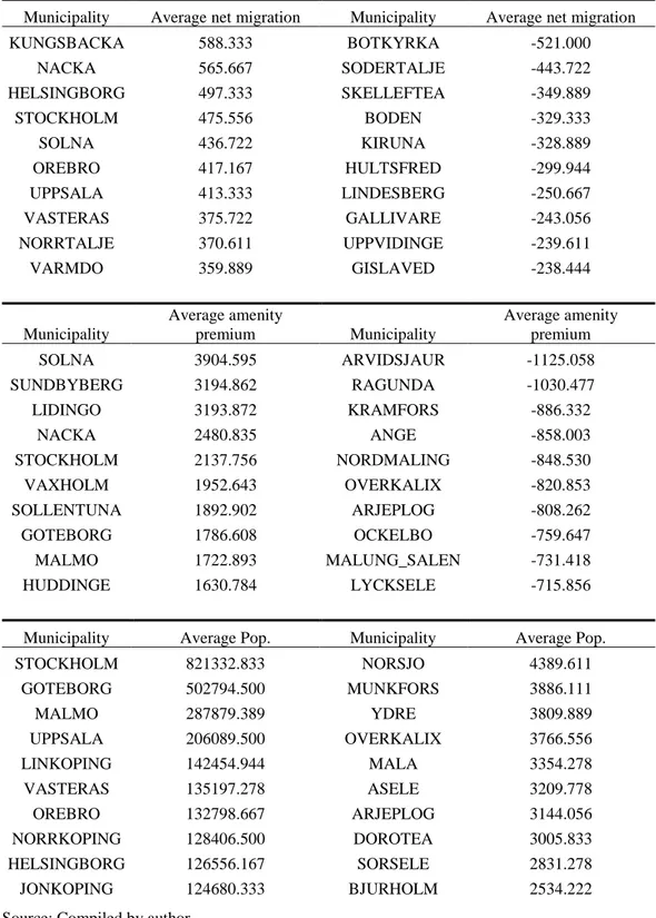
Table 4: Average; net migration, amenity premiums, and population for the period 1999 to 2016 for top
and bottom ten municipalities
Municipality Average net migration Municipality Average net migration
KUNGSBACKA 588.333 BOTKYRKA -521.000 NACKA 565.667 SODERTALJE -443.722 HELSINGBORG 497.333 SKELLEFTEA -349.889 STOCKHOLM 475.556 BODEN -329.333 SOLNA 436.722 KIRUNA -328.889 OREBRO 417.167 HULTSFRED -299.944 UPPSALA 413.333 LINDESBERG -250.667 VASTERAS 375.722 GALLIVARE -243.056 NORRTALJE 370.611 UPPVIDINGE -239.611 VARMDO 359.889 GISLAVED -238.444 Municipality Average amenity premium Municipality Average amenity premium SOLNA 3904.595 ARVIDSJAUR -1125.058 SUNDBYBERG 3194.862 RAGUNDA -1030.477 LIDINGO 3193.872 KRAMFORS -886.332 NACKA 2480.835 ANGE -858.003 STOCKHOLM 2137.756 NORDMALING -848.530 VAXHOLM 1952.643 OVERKALIX -820.853 SOLLENTUNA 1892.902 ARJEPLOG -808.262 GOTEBORG 1786.608 OCKELBO -759.647 MALMO 1722.893 MALUNG_SALEN -731.418 HUDDINGE 1630.784 LYCKSELE -715.856
Municipality Average Pop. Municipality Average Pop.
STOCKHOLM 821332.833 NORSJO 4389.611 GOTEBORG 502794.500 MUNKFORS 3886.111 MALMO 287879.389 YDRE 3809.889 UPPSALA 206089.500 OVERKALIX 3766.556 LINKOPING 142454.944 MALA 3354.278 VASTERAS 135197.278 ASELE 3209.778 OREBRO 132798.667 ARJEPLOG 3144.056 NORRKOPING 128406.500 DOROTEA 3005.833 HELSINGBORG 126556.167 SORSELE 2831.278 JONKOPING 124680.333 BJURHOLM 2534.222
Source: Compiled by author
Table 4 presents the average net migration, amenity premiums, and population for the top and bottom ten municipalities. The top ten positive net migration municipalities are a mix of: municipalities with a high average population (Stockholm, Orebro, Helsingborg,
20
Uppsala, Vasteras), municipalities that are growing in size (Kungsbacka) and municipalities that are relatively close to the capital, Stockholm (Nacka, Solna, Norrtalje, Varmdo). The bottom ten negative net migration municipalities are a mix of municipalities that are: north of Stockholm (Skelleftea, Boden, Kiruna, Lindesberg, Gallivaare), in close proximity to Stockholm (Botkyrka, Sodertalje) and southern Sweden (Hultsfred, Uppvidinge, Gislaved). These results suggest that Stockholm, the capital of Sweden, is an attractive area for people to move to. The high negative migration numbers for Botkyrka and Sodertalje are most likely due to people moving from these areas to other municipalities close to Stockholm.
Five out of the top ten positive net migration municipalities are also found under municipalities with the highest average population numbers. This suggests that municipalities that are initially bigger in size have a greater chance of attracting people towards the municipality. Therefore, if net migration is strongly dependent on population size and arenas are being built or renovated in those municipalities that have an initial high population size, then the correlation found between net migration and sports arenas could be an artificial one shadowing the true correlation between net migration and population size. In fact, five out of the ten top municipalities with positive net migration numbers have built or renovated an arena during the period of analysis (Orebro, Uppsala, Stockholm, Helsingborg, Solna). This means that the results could suffer from reverse causality or simultaneity, where instead of sports arenas having an impact on net migration, net migration could be impacting the building or renovation of sports arenas (reverse causality) or it could be the case that they are causing each other (simultaneity). Municipalities that feature within the top ten average amenity premiums are those that are close to Stockholm and included in their county (Solna, Sundvyberg, Lidingo, Nacka, Vaxholm, Sollentuna, Huddinge), and the three most populated cities in Sweden (Stockholm, Goteborg, and Malmo). These municipalities represent the most attractive places to live in when considering incomes and house prices. The bottom ten in this list, which represent the least attractive places to live, are municipalities north of Stockholm, which are typically sparsely populated, experiencing harsher climates than the rest of Sweden. The top and bottom ten municipalities listed in table 4 are good representations of those locations which have high and low amenities. From the top ten average amenity premium municipalities, three (Solna, Nacka, Stockholm) are also found in the top ten
21
positive average net migration list. This is in line with the literature, where it is has been seen that people move in search of locations with high amenities.
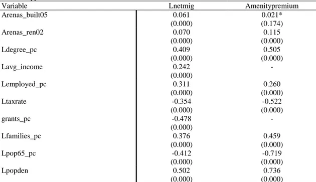
Correlation Analysis
Table 5 presents Pearson´s correlation matrix for the dependent variables, Lnetmig and amenitypremium, with the independent and control variables estimated for both models. Arenas_built05 records a small, positive relationship with Lnetmig but an insignificant relationship with amenitypremium. Arenas_ren02 portrays a relatively small positive relationship with both Lnetmig and amenitypremium.
Net migration’s strongest correlation value is with Lpopden. Net migration is positively correlated with arenas_built05, Ldegree_pc, Lavg_income, Lemployed_pc, Lfamilies_pc, and Lpopden, whilst a negative relationship is realised for Ltaxrate, grants_pc, and Lpop65_pc.
Amenitypremium’s strongest correlation value is with population density, Lpopden. Amenitypremium is positively correlated with Ldegree_pc, Lemployed_pc, Lfamilies_pc, and Lpopden whilst a negative relationship is realised for Ltaxrate and Lpop65_pc. All variables give the expected sign (see section 4.1.4).
The full correlation matrix (see appendix B) portrays high correlations between grants_pc and Lpopden, Ldegree_pc and Lavg_income, and Lfamilies_pc and Lpop65_pc. The greater the multicollinearity present the greater are the standard errors, meaning that it is harder for coefficients to be statistically significant (Alin, 2010).
22
Table 5: Pearson correlation table for variables included in models 1 & 2. Dependent variables are Lnetmig
and amenitypremium
Variable Lnetmig Amenitypremium
Arenas_built05 0.061 (0.000) 0.021* (0.174) Arenas_ren02 0.070 (0.000) 0.115 (0.000) Ldegree_pc 0.409 (0.000) 0.505 (0.000) Lavg_income 0.242 (0.000) - Lemployed_pc 0.311 (0.000) 0.260 (0.000) Ltaxrate -0.354 (0.000) -0.522 (0.000) grants_pc -0.478 (0.000) - Lfamilies_pc 0.376 (0.000) 0.459 (0.000) Lpop65_pc -0.412 (0.000) -0.719 (0.000) Lpopden 0.502 (0.000) 0.736 (0.000)
Note: figures in parenthesis represent probability values for t = 0. * Denotes insignificance at 5% level of acceptance. L refers to variables that are log transformed.
Regression Analysis
The regression analysis section begins with examining hypotheses 1 and 2 by estimating model 1, which is then followed by the estimation of model 2 in examination of hypotheses 3 and 4. Both models 1 and 2 are estimated using white period robust standard errors. White period robust standard errors assume that the errors for a cross-section are heteroscedastic and serially correlated. Since cross-sectional data with large differences between maximum and minimum values are realised (see section 5.1), then it is highly likely that cross-sectional heteroscedasticity is present. Serial correlation, although captured to some extent by including an AR(1) term, is still present in the residuals and thus validifies the use of white period robust standard errors. Furthermore, all FGLS estimations use cross-section weights, which assumes the presence of cross-section heteroscedasticity.
23
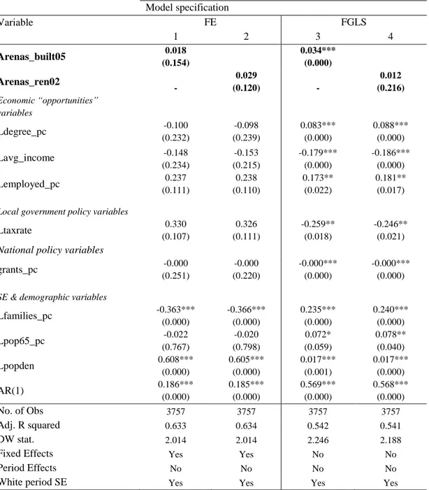
Table 6: Regression results using FE and FGLS estimation techniques. Dependent variable is Lnetmig.
Model specification Variable FE FGLS 1 2 3 4 Arenas_built05 0.018 (0.154) 0.034*** (0.000) Arenas_ren02 - 0.029 (0.120) - 0.012 (0.216) Economic “opportunities” variables Ldegree_pc -0.100 (0.232) -0.098 (0.239) 0.083*** (0.000) 0.088*** (0.000) Lavg_income -0.148 (0.234) -0.153 (0.215) -0.179*** (0.000) -0.186*** (0.000) Lemployed_pc 0.237 (0.111) 0.238 (0.110) 0.173** (0.022) 0.181** (0.017)
Local government policy variables
Ltaxrate 0.330 (0.107) 0.326 (0.111) -0.259** (0.018) -0.246** (0.021)
National policy variables
grants_pc -0.000 (0.251) -0.000 (0.220) -0.000*** (0.000) -0.000*** (0.000)
SE & demographic variables
Lfamilies_pc -0.363*** (0.000) -0.366*** (0.000) 0.235*** (0.000) 0.240*** (0.000) Lpop65_pc -0.022 (0.767) -0.020 (0.798) 0.072* (0.059) 0.078** (0.040) Lpopden 0.608*** (0.000) 0.605*** (0.000) 0.017*** (0.001) 0.017*** (0.000) AR(1) 0.186*** (0.000) 0.185*** (0.000) 0.569*** (0.000) 0.568*** (0.000) No. of Obs 3757 3757 3757 3757 Adj. R squared 0.633 0.634 0.542 0.541 DW stat. 2.014 2.014 2.246 2.188
Fixed Effects Yes Yes No No
Period Effects No No No No
White period SE Yes Yes Yes Yes
Note: figures in parenthesis represent probability values for t statistics. L refers to variables that are logged transformed, _pc refers to variables in per capita form. ***Denotes significance at 1% level, **Denotes significance at 5% level, *Denotes significance at 10% level.
The total number of observations in table 6 is less than 5202 which is the number of observations if the panel were to be balanced. The reason for this is that data for some variables included in model 1 is not available over the full time period which means that observations are lost. The results in table 6 depict different results for arenas_built05 depending on the estimation technique used, whilst arenas_ren02 depicts insignificance regardless of estimation technique. The FGLS estimates in column 3 show a small,
24
positive and significant relationship between arenas_built05 and Lnetmig whilst the FE estimates in column 1 portray an insignificant relationship. Column 3, shows significance for all independent and control variables in the model. Lavg_income and Lpop65_pc depict contrary relationships to what was found in the correlation analysis. These results might be due to the high collinearity present amongst other explanatory variables (see appendix B). To tackle this, Ldegree_pc, Lfamilies_pc, and grants_pc are removed from model 1 and model 1 is re-estimated (see appendix D, table 1). The results show that Lavg_income becomes positive and insignificant in the FGLS regression, and negative and significant in the FE regression, which still means that the variable portrays unexpected results. Lpop65_pc becomes negative and significant using FGLS estimation which is line with the literature and supports the claim of multicollinearity present between the control variables in table 6. Variables arenas_built05 and arenas_ren02 maintain the same relationships after the removal of the collinear variables. Arenas_built05 in column 3 shows a slightly smaller coefficient than in table 6 (see Appendix D, table 1).
The other control variables in table 6, besides grants_pc, give expected results, with Lfamilies_pc showing the highest positive relationship with Lnetmig. Grants_pc depicts no relationship with Lnetmig which is not in accordance with what was found in the Pearson correlation table in table 5 of a relatively high negative relationship.
25
Table 7: Regression results using FE and FGLS estimation techniques. Dependent variable is
amenitypremium. Model specification Variables FE FGLS 1 2 3 4 Arenas_built05 -2.795 (0.905) 8.818 (0.659) Arenas_ren02 - -19.643 (0.547) - -21.953* (0.084) Economic “opportunities” variables Ldegree_pc -603.929*** (0.000) -602.471*** (0.000) 561.302*** (0.000) 562.609*** (0.000) Lavg_income - - - - Lemployed_pc -284.093*** (0.000) -284.135** (0.038) -478.602*** (0.000) -477.598*** (0.000)
Local government policy variables
Ltaxrate 205.972 (0.608) 207.308 (0.605) 1564.535*** (0.000) 1564.230*** (0.000)
National policy variables
grants_pc - - - -
SE & demographic variables
Lfamilies_pc 489.016* (0.056) 489.577* (0.056) 210.605** (0.029) 211.139** (0.029) Lpop65_pc -2493.350*** (0.000) -2492.358*** (0.000) -1768.888*** (0.000) -1777.352*** (0.000) Lpopden 689.754*** (0.001) 690.344*** (0.001) 647.137*** (0.000) 647.055*** (0.000) AR(1) 0.773*** (0.000) 0.773*** (0.000) 0.973*** (0.000) 0.973*** (0.000) No. of Obs 3757 3757 3757 3757 Adj. R squared 0.968 0.970 0.976 0.976 DW stat. 2.238 2.239 2.335 2.334
Fixed Effects Yes Yes No No
Period Effects No No No No
White period SE Yes Yes Yes Yes
Note: figures in parenthesis represent probability values for t statistics. L means that the variable has been log transformed, whilst _pc means that the variable has been divided by total population. ***Denotes significance at 1% level, **Denotes significance at 5% level, *Denotes significance at 10% level
To test hypothesis 3 and 4, model 2 is run. The results in table 7 show no significant relationship in all estimation techniques for arena_built05 whilst a negative significant relationship is recorded for arena_ren02 in column 4 with FGLS estimation. This result suggests that a renovated sports arena decreases the attractiveness of a municipality. Lemployed_pc and Ltaxrate portray opposite relationships to what was expected in section 4.1.4 and what was found in table 5. This again could be due to the multicollinearity present amongst variables (see appendix B). To check whether this is the case, Ldegree_pc is removed from the equation along with Lfamilies_pc and model 2
26
is re-run again (see appendix D, table 2). Lemployed_ pc becomes insignificant using FE estimation but remains unchanged in sign and significance when estimated by FGLS. Ltaxrate becomes positive and significant when employing FE estimation and remains positive and significant in the FGLS regression. This does not support the claim that multicollinearity affects the results in table 7.
6. Analysis of Results
The assessment of empirical results starts with the first hypothesis which stated that a sports arena built in municipality i at time t is positively related to net migration in year t + 5 for the same municipality. Results reported in table 6 show a small, positive and significant relationship between arenas_built05 and Lnetmig using FGLS estimation techniques, however, FE estimation produces an insignificant result. This could either mean that despite the Hausman test suggesting the use of FE estimation the technique does not fit the data or that arena_built05 is truly insignificant and FGLS estimates are biased. Past studies have found that when including a lagged term of the dependent variable, which is indirectly done in the regressions by including an AR(1) term, FE estimation produces asymptotically biased results as the demeaning process of an FE estimation creates a correlation between independent variable and error (Nickell, 1981). This means that one is more inclined to trust the FGLS results in table 6. The positive and significant relationship between arenas_built05 and Lnetmig means that five years after the building of a sports arena in municipality i, net migration is set to increase by 3.45% in year t + 5. This result is important to keep in context, as building an arena in a remote area with no proximate attractions is unlikely to attract people to the municipality where the arena is built. Furthermore, the sports arenas studied in this paper are being used by football and ice hockey teams that compete in the highest and second highest leagues. The fact that football and ice hockey are the two main sports in Sweden and data on sports arenas is collected for teams in the higher echelons of their respective sport requires consideration when interpreting the results. Most municipalities that have had an arena built during the period 1999 to 2016 for the teams analysed in this study are municipalities such as Boras, Malmo, Goteborg, Stockholm, and Solna which are population dense municipalities. Therefore, once again, the notion of reverse causality, where instead of the building of sports arenas having an impact on net migration, net migration could be
27
impacting the building of sports arenas and simultaneity, where the building of sports arenas and net migration cause each other, should also be kept in mind when interpreting the results.
This paper is one of the first to find a significant relationship between a newly built sports arena and net migration. Värja (2014) analyses the relationship between the municipal sports environment and the net migration rate and finds no significant relationship except when the author removes Stockholm, Goteborg, and Malmo from the analysis.
The second hypothesis stated that a sports arena renovated in municipality i at time t is positively related to net migration in year t + 2 for the same municipality. Results in table 6 show no significant relationship between arenas_ren02 and Lnetmig for both estimation techniques (FE and FGLS). This result therefore rejects the hypothesis. Furthermore, this result indicates that renovating a sports arena does not generate enough interest from individuals outside the municipality to consider moving into the municipality where the arena is being renovated. However, a point to note is that due to the lack of data available on renovation cost, both smaller and larger type renovations were included in the analysis. If the renovation cost was known, and one would be able to distinguish between smaller and larger renovations then the analysis for hypothesis 2 could be enhanced.
The third hypothesis stated that municipalities that have a sports arena built realise positive amenity premiums five years later. Whilst the fourth hypothesis stated that municipalities that have a sports arena renovated realise positive amenity premiums two years later. Table 4, in the descriptive statistics, produces encouraging results for the third hypothesis. Four municipalities that feature within the top ten, for municipalities with the highest amenity premiums, have had an arena built during the period 1999 to 2016. The regression results in table 7, however, show insignificant results for arena_built05 and a negative relationship between arena_ren02 and amenitypremium. The third and fourth hypotheses are thus rejected. The very high adjusted R2 in table 7 suggests that the results depicted could be more of an econometric issue rather than an actual insignificant relationship between the two sports arena presence dummy variables and amenitypremium.
28
7. Robustness Diagnostics
As robustness checks for arena_built05 and arena_ren02, the three most populated municipalities, Stockholm, Goteborg, and Malmo are excluded from both dummy variables. Being the three most populated municipalities with large labour markets their attractiveness in drawing people into the municipality is assumed to be greater than other municipalities. Moreover, these three municipalities have had more than one sports arena built during the time period analysed and therefore might attract individuals to a greater extent than a municipality that has only one sports arena. Furthermore, Värja (2014) also removes these three municipalities for similar reasons from her analysis. Models 1 and 2 are re-run again and a decrease in coefficient estimates is expected for both variables due to the positive average net migration flows and the high attractiveness of these cities (see table 4).
The results show (see appendix E, table 1), on the contrary to what is expected, higher coefficient estimates for arena_built_nomajor05 when model 1 is re-run in column 3. When taking a closer look at the data, although these three municipalities have positive average net migration flows, both Goteborg and Malmo record negative net migration flows five years after a sports arena was built whilst Stockholm did not affect the results as ‘Tele2 Arena’ was built in 2013 which means that a time gap of five years does not capture the effects for Stockholm’s arena. Arenas_ren_nomajor02, using FGLS estimation in column 4, depicts a small, positive and significant estimate however the estimate in column 2, using FE estimation, remains insignificant. This result means that sports arenas that have been renovated outside Stockholm, Goteborg and Malmo municipalities experience a small positive net migration flow two years after renovation. When re-running model 2 (see appendix D, table 2), the results show insignificant results for both arenas_built_nomajor05 and arenas_ren_nomajor02.
Another robustness check is made by eliminating the time assumptions for a newly built and renovated arena to realise a relationship with net migration and amenity premiums. A sports arena built or renovated is now assumed to affect net migration and amenity premiums the same year. When estimating model 1, the results (see appendix E, table 3) show insignificant results for both arenas_built and arenas_ren for all estimation
29
techniques except in column 2 using FE estimation. The results in appendix E, table 3 support the assumption of a five year time delay for sports arenas built to realise a relationship with net migration, whilst the justification for the assumption of a two year time delay for sports arenas renovated to have an impact on net migration is more ambiguous. Re-estimating model 2 (see appendix E, table 4) displays insignificant results for both arenas_built and arenas_ren.
8. Conclusions
The purpose of this paper has been to examine the impact of the building or renovation of a sports arena on net migration and amenity premiums by analysing 289 Swedish municipalities for the period 1999 to 2016. To limit the collection of data on sports arenas in Sweden, information has been gathered for sports arenas that were being used by football and ice hockey sports teams in the highest and second highest league. This means that a total of 57 sports arenas have been analysed. Out of those 57 arenas, 21 arenas have been built and 33 have been renovated over the time period 1999 to 2016.
The majority of sports arena studies have focused on post-construction employment and/or income effects (Richardson, 2016; Santo, 2005; Coates and Humphreys, 1999). This study is one of several studies investigating the non-monetary effects of sports arena construction and renovation. Moreover, this paper is one of the few to investigate the relationships between sports arenas and net migration along with sports arenas and amenity premiums.
The results show that a municipality that has a sports arena built in year t, experiences a 3.458% increase in net migration in year t + 5. Furthermore, a small positive significant relationship is found between sports arenas renovated and net migration when Stockholm, Goteborg, and Malmo are removed from the analysis. FE and FGLS estimation techniques produce no significant results for the relationship between amenity premiums and municipalities with sports arenas, whether built or renovated.
Future studies on this topic could build on this study by including each yearly five year lag on the sports arena dummy variable, arenas_built, to find out how and if the relationship between the dependent variables, net migration and amenitypremiums, and arenas_built05 changes. Another suggestion if pursuing this topic is to use different
30
regression estimation techniques such as dynamic panel estimation and to include measures to account for spatial dependence which is a common occurrence in geospatial analysis such as the one undertaken. A different avenue to take would be to investigate the relationship between sports arena construction or renovation on housing prices. There are several authors who have studied this field of research, however, a Swedish study on this topic is yet to be seen.
9. References
Abrams, J. & Gosnell, H. (2009), “Amenity migration: diverse conceptualizations of drivers, socioeconomic dimensions, and emerging challenges”, GeoJournal, Vol. 76, No. 4, pp. 303 – 322.
Ahlfeldt, G. & Maennig, W. (2008) “Impact of sports arenas on land values: evidence from Berlin”, The annals of regional science, Vol. 44, No.2, pp. 205 -227.
Ahlfeldt, G. & Maennig, W. (2010), “Stadium Architecture and Urban Development from the Perspective of Urban Economics”, International Journal of Urban and Regional
Research, Vol. 34, No. 3, pp. 629 – 646.
Anzilotti, E. Citylab. (2016). Should the federal government be funding private sports
stadiums?. Retrieved 2018 February 20 from
https://www.citylab.com/solutions/2016/09/quantifying-the-federal-dollars-spent-on-sports-stadiums/499856/
Alin, A. (2010), “Multicollinearity”, Wiley Interdisciplinary Reviews: Computational
Statistics, Vol. 2, No. 3, pp. 370 – 374.
Aronsson, T. et al. (2001), “Regional Income Growth and Net Migration in Sweden, 1970‐1995”, Regional Studies, Vol. 35, No. 9, pp. 823 – 830.
Austrain, Z. & Rosentraub, M. (2002), “Cities, sports and economic change: a retrospective assessment”, Journal of Urban Affairs, Vol. 24, No. 5, pp. 549 – 563.