J
Ö N K Ö P I N GI
N T E R N A T I O N A LB
U S I N E S SS
C H O O LJÖNKÖPING UNIVERSITY
C o m m u t i n g pa t t e r n s i n S w e d e n
A study of commuting, education and functional regions
Bachelor thesis within Economics Authors: Johanna Eliasson
Michael Ström
Tutors: Professor Charlie Karlsson Ph.D. candidate Lina Bjerke Jönköping February 2008
Bachelor’s thesis within Economics
Title: Commuting patterns in Sweden – A study of commuting, education and functional regions
Authors: Johanna Eliasson Michael Ström
Tutors: Charlie Karlsson, Professor Lina Bjerke, Ph. D Candidate Date: 2008-02-12
Keywords: Commuting, education, human capital, and functional regions JEL-codes: R12, R14, R23, and R40
Abstract
Eurosclerosis is gripping Europe; one suggested remedy is higher mobility of people. That is what this thesis aims to address: Inter-municipality commuting mobility in Sweden. This essay is investigating the Swedish commuting as of 2005. The hypothesis is duly formed as such: High education is significant for the outcome of the commuting decision. The regional pattern of commuting is also considered to a degree. Aggregated data on Swedish commuting between municipalities is used.
The theory used to investigate this is basic agglomeration theory including the simplest form of gravity model. Theories on utility, human capital and distance friction complement the analysis.
Concluding comments include: higher education is significant for the commuting decision, and living in more densely populated areas like “big” cities increases chances of people commuting.
Table of Contents
1
Introduction... 1
1.1 Research problem ...2
1.2 Purpose ...2
1.3 Disposition of the thesis...3
2
Theories of commuting ... 4
2.1 Monocentric model, agglomeration and commuting ...4
2.1.1 Agglomeration and commuting...6
2.2 The utility of commuting...7
2.3 Investing in human capital ...9
2.3.1 Distance friction and time sensitivity of commuting ...9
2.4 Summary ...11
3
Method ... 12
3.1 Gravity model ...12
3.2 Functional regions and commuting...12
4
Empirical findings and analysis... 14
4.1 The data ...14 4.2 Estimation models ...15 4.2.1 Statistical errors...16 4.3 Result ...17
5
Analysis ... 20
6
Conclusion ... 22
References ... 23
Appendices ... 25
1 Introduction
Today it is a fact that emerging economies’ growth outpaces European economies by leaps and bounds. Eurosclerosis seems to be endemic and governments need to look at ways to “snap out of it”. Geographical movement is said to promote economic growth. The geo-graphical movement in Sweden has traditionally been low compared to other developed countries which in turn is likely to have something to do with the population density in Sweden which is, and has historically been, low, a fact which would today probably promote a higher level of geographical movement of people, either through migration or commut-ing.
Everyday some 1.3 million people in Sweden cross a municipal border(s) to a different mu-nicipality than they reside in to go to their job. This constitutes about 30 per cent of the whole Swedish labour force (SCB, 2005). As visible from this number the commuting in Sweden is an extensive phenomenon and reflects the history of Sweden in the sense of ur-banisation and politics. This commuting over municipal borders is possibly a consequence of the late urbanisation which did not take place until long after many other countries in Europe.
The concept used in this thesis is commuting or commuter. This refers to an individual em-ployed by a company or an organisation residing outside the individual’s home region (the individual’s municipality of residence). Sometimes the word household will appear in the text; this term is only used unscientifically as a synonym for more than one person living under the same roof. By commuting furthers refer to the short distance commuting that takes place between municipalities and not long-distance commuting across different LA-regions1. Another concept used in this thesis is geographical labour mobility which can actually be divided into three different dimensions, but this thesis will focus on one of them: the change of workplace (Eliasson et al., 2003). The other two concepts are i) a residential change and ii) a transition between labour market states. The former concept being some-what outside the scope of this thesis because of the limit (the thesis only deals with com-muting, not migration) imposed on the thesis. The latter presents a significant factor on commuting outcomes, and although it is not what is focused on here, it is however men-tioned, for the sake of giving perspective.
There are different ways to approach the topic of commuting; one interesting plan of at-tack is to compare perceived and real differences between the sexes. On the other hand it has been argued in some quarters that the perceived difference between the genders is ac-tually one of education; men tend to be, still, more educated than women of the same age and background. It would be interesting to see if level of education as a variable is influen-tial for the dependent variable of commuting.
Since the infrastructural quality has improved in Sweden over the years, and with that (by logic assumption) the public transportation system, commuting as a viable option has in-creased and is now in some cases a substitute for moving, which in its own way has some beneficial aspects to it, such as avoiding housing market restrictions (Westerlund, 2001). The infrastructure has increased in both kilometres (km) and quality, and the average mo-bility of persons has also increased, from only a half km in 1900 to 45 km in 1999
1 Functional regions in Sweden are often referred to as LA-regions (lokala arbetsmarknader) as specified by
son and Strömquist, 1988 cited in Olsson, 2002). Since 1970 there has been an increase in the commuting from 500 000 people to almost 1 million at the end of the 1990s (Lindgren, Eliasson and Westerlund, 2002). This increase in commuting by 100 percent is one out of a number of interesting facts that make this topic worth looking into since one can see an in-creasing trend in commuting and surely would expect that this trend will continue on in the future. This increase in mobility makes investigating the patterns of commuting important.
1.1 Research problem
Even though the infrastructure has become better, the individual’s upper limit of commut-ing in Sweden is somewhere around 60 minutes, after that, workers will start to think about other possibilities such as weekly commuting (Olsson, 2002) or even migrating to another area. An upper limit clearly exists, and that limit is critical to the decision of migrating or commuting. Olsson’s (2002) dissertation contains 4 articles that discuss commuting in the region of Fyrstad. The effect of education on commuting with a simultaneous change in the infrastructure is addressed in this dissertation. He concludes that there are visible dif-ferences in the commuting patterns of different education groups (classes of low, medium or high education). Olsson also mentions the difference between men and women con-cerning education and distance friction, the latter being lower for men, with no effect of this kind detected for women.
Eliasson et al. (2007) have made a study on both migration and commuting and its effect on the income in Sweden. They have made an analysis of the geographical mobility between the LA-regions in Sweden during the last 30 years and conclude that geographical mobility has increased during that time.
This study limits itself to the commuting patterns in Sweden and there are several reasons, according to Westerlund and Wyzan (1995), why Sweden is a good focus for a study like this. One argument is that the size of the public sector relative to the gross domestic prod-uct (GDP) is one of the largest in the world; there is also a lot of highly detailed data on households. Sweden additionally shows a spatial structure of both large metropolitan areas, such as Stockholm, Gothenburg and Malmö and also areas with some of the world’s lowest population densities, up in the north (in the region of Norrland) this problem is also brought up in the thesis. All these limits contribute well to the thesis’ purpose.
Since commuting is a phenomenon for working people, it puts another limit to the thesis and it also has to limit the analysis to those who are employed. When looking into patterns of commuting, this thesis assumes that the opportunity of migrating has already been thought of and also rejected because of the costs outweighing the benefits. The assump-tions made in this thesis will be in the short-run.
1.2 Purpose
The purpose of this thesis is to analyse certain characteristics of commuting flows in Swe-den, and in particular if there is a difference between urbanized and less urbanized regions, and to what extent the level of education influences the commuting flow.
1.3 Disposition of the thesis
The following chapter is the foundation for the analysis and conclusion with its commuting theories such as agglomeration, utility and distance friction.
Chapter 3 deals with how the data is shaped and fitted into the regression model; there is also a short discussion of the functional regions and its significance.
Chapter 4 is dedicated to the data and how it has been retrieved, and also the empirical re-sult.
Chapter 5 presents the analysis of the result.
The sixth and last chapter is a concluding chapter with some suggestions for further studies within this topic.
2 Theories of commuting
The idea of this chapter is to present some of the most basic ideas and theories concerning commuting and how it can be explained by agglomeration through economies of scale effects and utility maximisa-tion. There are also discussions about how the time and distance will affect the individual in choosing to commute or not. The theory will be discussed and analysed with the help of empirical findings later on in the thesis.
2.1 Monocentric model, agglomeration and commuting
The earliest models concerning commuting hail from the work of, among others von Thünen (Figure 2-1) (1826, cited in Brakman, Garretsen & Marrewijk, 2001). Still a bench-mark model for work in urban and regional economics, the monocentric model primarily describes commuting patterns when there are no increasing returns to scale. Although it was later, by Alonso (1964) modified to incorporate commuting as its main theme, the monocentric model at first focused solely on a so called bid-rent approach with a perfectly homogenous city (cited in Brakman et al., 2001). Farmers living outside of this city would then bid on the rent of living as close to the city as possible (Figure 2-1), being able to pay rent equal to their received income from their respective crop type. Each farmer wants to minimize transport costs, and the model thus represents a trade-off between land rents and transport costs.
2-1 von Thünen model
D is ta n c e fr o m c ity c e n tre B id -r e n t c u rv e s f lo w e r s v e g e t a b le s g r a in A B fl o w e r s v e g e ta b l e s g r a i n
Source: Brakman et al.
Alonso (1964) substituted farmers for commuters living around a city with a Central Busi-ness District (CBD). In this Central BusiBusi-ness District, commuters place value in living closer to the areas closer to the Central Business District, that is, they place utility in living closer to economic activity due to transport costs. On the other hand rents are higher the closer to the centre the commuters live. Commuters must then contend with other
com-muters whose willingness to live close to the centre as well forces a bid-rent scheme where people living closer to the centre pay more than do “outliers”. Just as in the farmer version of the monocentric model, this then leads to an efficient allocation of land, where the commuters most willing to pay for it, decide the use of land (effectively moving there so as to lay claim to their plot of land).
In a utility framework, the perceived utility (U) results in a convex relation where utility is dependent on the consumption of goods (X) and space (S), so the function is U(X, S). The slope of the bid-rent curve in Figure 2-1 is given by t/S where t is the transport cost per good and S is the number of land units for production.
Each individual (be he or she a commuter or a firm) tries to maximise the received and per-ceived utility by moving as close as possible to the centre. This is however subject to a budget constraint. Each commuter thus tries to maximise his utility given this budget con-straint, that is, an effective allocation of land is where the budget constraint is tangent with the slope of the bid-rent curve in the monocentric model.
2-2 simplified von Thünen model
Source: Brakman et al.
This monocentric model also shows how the individual always tries to minimise his/her commuting costs. The monocentric model has, unfortunately, shown not to be in line with empirical studies and they show that people are actually commuting longer and to a higher cost than what is necessary. When the individual chooses where to work and live he/she will most likely pay some attention to the commuting costs. Wasteful commuting, to use Hamilton’s (1982) terms, or excess commuting is everything beyond what, on an average, is needed to commute between work and the residential area (Small & Song, 1992). Hamilton (1982) was the first to look for inefficiencies in the commuting patterns. He shows that the monocentric model, when it is modified for decentralised employment, predicts that the individual will choose a utility maximising location that also minimises the aggregate com-muting distance. But the findings he made from his investigation of 14 major cities in the US in 1972 showed the opposite result. The actual commute was about eight times the minimised average predicted by the monocentric model.
In early versions of the monocentric model, perfect competition is assumed and the central premise is that land and living costs are decreasing functions of distance. When the
indi-Flowers
Vegetables
vidual decides the residence location, travelling costs are also decided upon. When choos-ing where to live, the individual is expected to always maximise his/her utility (discussed in Section 2.2), so increased travelling costs can be traded against increased consumption of goods and living area. Here, commuting can be applied to this early model. When an indi-vidual decides where to live he/she will make a calculation of the different costs. If he/she decides to move further out from the CBD that person will have a lower land rent but a higher commuting cost when it has to go to work, on the other hand, if the person decides to live close to the CBD it will experience a higher land rent but a lower commuting cost. The latter versions of the model have left the assumption of a Central Business District and are instead trying to decide the forming of the centre (or agglomeration) inside the model (Eliasson et al., 2007).
2.1.1 Agglomeration and commuting
Fujita and Thisse wrote in 1996 (p. 340): “agglomeration can be found in the existence of strong regional disparities within the same country, in the formation of cities having differ-ent sizes, or in the emergence of industrial districts where firms have strong technological and/or informational linkages.”
Scale economies are often thought of as one of the most determining reason for agglomera-tion, there are also reasons such as better matching efficiency for the demand and supply, a more efficient way of spreading knowledge and a higher pace-setting for innovations. Glae-ser (1994) argues that there are external positive economies of scale, namely in the form of cumulative effects of knowledge. Glaeser (1994) argues for a positive correlation between the accumulation of knowledge (here presented in its most basic, measurable version: edu-cation) and the continued growth of an economy. Given an already positive trend as far as education is concerned, one can expect to see even more growth for the industry at hand. Now, this is a bit premature to say since the empirical evidence toward this conclusion is a bit thin, and could almost just as well be explained by neo-classical theory and first-nature assumptions of natural advantages.
Figure 2-3 shows the mechanics of agglomeration in two different regions. Point A shows full agglomeration in region 1 and point E shows full agglomeration in region 2. In be-tween these two extremes one can find different degrees of agglomeration, point B shows that approximately 80 per cent of the population lives in region 1 while the rest of the population lives in region 2, the same is for point D but the largest part of the population lives in region 2. Point C is where there is almost an even spread over the two regions.
w1/w2
λ1
2-3 the core model
Source: Brakman et al. 2001
As Parr (2002) suggests in his paper, agglomeration economies can be seen as a decrease in the unit cost of a firm, being the result of economic activity concentrating in a given loca-tion. In more general terms, there are different types of agglomeration economies. As de-fined by Parr, sorted by different dimensions: namely economies of scope; scale or com-plexity; and either internal or external to the firm. The common denominator here regard-less of the type of agglomeration economy, is the concentration of economic activity, and given that people live away from where they work (which it is here posited that they tend to do), it then implies some kind of spatial separation between working areas and residen-tial areas. This opens up for commuting, provided that there is enough utility to be gained. Commuting also implies a commuting cost since proximity in itself is negatively correlated with transport cost.
The most straightforward of the different types of agglomeration economies is the econo-mies of scale of the core model, which addresses more explicitly the manufacturing type of firm. It is the scale economies and the commuting costs that determine the optimal size of cities in an economy. The economies of scale will force the creation of larger cities but it will be held back by the increasing commuting costs (Eliasson et al., 2007).
2.2 The utility of commuting
Commuting is assumed to be dependent on the variance of utility which is a measure of satisfaction when consuming a good or service. If a good or service generates higher utility, then consuming more of that good or service will increase the individual’s utility. Commut-ing will then only occur when the utility of commutCommut-ing is higher than the utility of movCommut-ing and working nearby since it is a goal for every individual to maximize his/her utility (Bade & Parkin, 2004). People will always strive to reach a higher utility level than before. In this case it is important for the individual or the household to find the localisation that will maximise his/her utility or welfare (Eliasson, et al., 2007).
The budget lines are constraining the consumption possibilities of good X and Y. The curved indifference lines are the curves along which the individual is indifferent to the
dif-A
C D E
ferent combinations of consumption bundles of X and Y, that is, the individual does not prefer one combination over another. An individual will also get the same utility along that indifference curve. The further away the indifference curve is from the origin the higher amount of utility is obtained (Varian, 2003).
In the utility Equation 2-1, where on the left hand side of the equation UC is utility of com-muting, CCM is the parameter for the monetary cost of commuting and Ct is the time “cost”, the time spent on travelling,. On the right-hand side, the utility of not commuting, UNC resides. The utility on the left-hand side needs to be larger or equal to the utility on the right-hand side for commuting to take effect.
NC t M C C C C U U − − ≥ (Equation 2-1)
UC is the utility derived from the wage offered at the second location. To make the decision of starting to commute the individual needs some incentive to start reconsidering the cur-rent workplace and ancillary commuting pattern, both of which happen to be located in the same municipality as the place of residence. To work outside the municipality of residence and changing the commuting pattern to reflect this, in short, implies commuting. In effect, an individual revaluates previous choices and looks at what he/she has got now and what can obtained if he/she starts to commute. Wage premium (including all the benefits of-fered by the new employer) is a good variable for the likelihood to take a new job since workers are always searching for higher-paying jobs (Borjas, 2005).
There is also a time variable that should be considered. For the commuter there will be a lot of time spent in a car or other means of public transportation while the non-commuting person will have that same amount of time to spend on something else, like leisure, quality time with the family or spending time searching for a higher paying job inside the bounda-ries of his current community. This is all something that the commuter has to take into ac-count when forgoing current earnings from his/her current job in order to acquire a better pay-check given that workers maximize the net present value of income. The utility vari-ance, then, shows exactly when it would be advantageous for a resident in a given munici-pality to become a commuter. The utility function 2-1, in this way, shows the “break-even point” for starting to commute for a resident who puts a value on when deciding to com-mute or not.
Mentioned above and affecting a person very much, family ties and other social contacts are important aspects of utility and commuting. For married couples or couples living to-gether the choice of residence area is seen as a compromise that is maximising the house-hold’s total exchange from choosing between a number of conceivable localisations. If one person in a couple needs to move with his/her partner to another location that is not op-timal from an individual utility maximising perspective it is called a tied mover. If one of the partners is staying on a location because of his/her partner, it is called a tied stayer. When looking at these two scenarios, commuting can also be an outcome of a compromise be-tween spouses (Eliasson et al, 2007 and Mincer, 1978).
Part of the choices, of commuting or not, made by a household depend on the construc-tion of the household; is it a one-person household or a multiple-person household? Are there children living in the household? Just as for capital, households are considered to be fixed, a decision to move includes efforts like selling the house, finding a new house at the new location, and all of these different steps are considered to take up so much time that it cannot be viewed as a short-run decision, and therefore will not be paid much attention here. There are also other impediments for the ones who live in the household, they have
to find a new job and if there are children living in the household they have to be intro-duced to a new school. Another loss for the household is the social network of close fam-ily, friends and colleagues.
One thing that must not be forgotten is also the actual cost of commuting, the above men-tioned time spent on commuting is a cost, but one has to be aware of the monetary cost as well. There is a ticket cost when using public transportation, or, when using a car – the fuel cost. This cost could, in general senses, be reduced with infrastructure investments (Ols-son, 2002).
2.3 Investing in human capital
According to Schultz (1961) economists have known for long that people are important for increasing the wealth of nations. Many economists explain the rapid economic growth in Southeast Asia as an effect of an increase in human capital. Without any growth in human capital, argues Schultz (1961), there would only be hard manual work and poverty, accept for those who earn money from properties. Becker, Murphy and Tamura (1990) confirm Schultz’s way of thinking but not to the same extreme extent; they argue that there is now quite strong evidence for the link between investment in human capital and growth. Invest-ing in human capital can entail such thInvest-ings as schoolInvest-ing and on-the-job trainInvest-ing. This thesis is focusing on the former way of investing since the formal education is the easiest to measure.
Commuting is a way for the individual to increase the value of his/her human capital when the individual makes a choice to look for a job in another municipality to get a higher wage than before, or just to improve the individual’s future opportunities (Eliasson et al., 2007). The human capital theory has been developed from the neoclassical economical theory, in-stead of only focusing on the understanding of maximising the wage the analysis is broaden to also include both the monetary and non-monetary factors (Lindgren, Eliasson and Westerlund, 2002). Education also probably implies an individual to be more aware of ac-tual job openings in the commutable vicinity. Appendix Figure 1 from the Glaeser (1994) article shows the relation between income growth and the percentage of college-educated in 1960. There is a correlation between the level of education and the level of agglomera-tion in a region: human capital generates growth, which leads to more firms setting up shop in a region. An industry with low levels of education would not grow substantially when compared to other industries with higher numbers of educated.
2.3.1 Distance friction and time sensitivity of commuting
The distance between two places creates a friction, and individuals are facing differences in sensitivity towards these frictions. It is not only the labour market (even though the spatial distances plays a key role there) that is affected by this friction, hardly no markets are unaf-fected by this phenomenon. Theory states that friction sensitivity decreases the higher edu-cation one attain (Johansson, Klaesson and Olsson, 2002).
Something that can also be connected with distance friction is the time sensitivity of differ-ent individuals. One explanation to why it differs between individuals is the choice of type of job and by that also the wage structure. Individuals can face differences in sensitivity towards distance friction. A high time sensitivity implies that extra travel time will reduce the flow of commuters more so than low time sensitivity would do, logically it will be these not so sensitive people who commute (Johansson, Klaesson and Olsson, 2002).
2-4 Time sensitivity
Source: Johansson et al. 2002
Figure 2-4 shows the time sensitivity in commuting (the data is collected from Jönköping and its neighbouring municipalities), and according to Johansson et al. (2002) the ness to commute is decreasing with the travel time. After around 45 minutes the willing-ness is down to very low levels and one can conclude that the limit for commuting lies around the vicinity of 45 minutes. Even though the infrastructure has become better, the individual’s upper limit of commuting in Sweden is somewhere around 60 minutes, after that, workers will start to think about other possibilities such as weekly commuting (Ols-son, 2002) or even migrate to another area. This means that there is a limit to commuting and that limit is critical to the decision of migrating or commuting.
From empirical observations from Johansson, Klaesson and Olsson (2003) it is seen that distance is influencing commuting in a non-linear way meaning that the sensitivity is lower for short and long distances but distances that are defined as intermediate show a high time sensitivity. This can also be seen in Figure 2-4 with its S-shaped curve which starts with an almost flat part where the short distances are represented, after that the curve begins to fall quickly around the intermediate distances. This behaviour has been observed in a large number of the Swedish municipalities by Johansson et al. (2002).
2.4 Summary
This preceding chapter has described the different theories that this thesis will utilise when analysing the empirical findings. The theories focus on the spatial part of the problem with the theories of agglomeration, monocentric model and time- and distance sensitivity of the commuters as the main tools. All of the theories are relevant since they describe how an individual makes his/her choices with the respect to the environment around them, how they will make use of the utility to gain the most. With the help of the presented theories the authors hope not to reject the null hypothesis: commuting flows is increasing with the level of education. A secondary hypothesis is looked into; more densely populated regions experience more commuting. By looking at how the individual is investing in human capital one can see the patterns of how an educated person makes choices to maximise utility. This is seen as the main purpose of the thesis but there are also some other interesting as-pects in the commuting behaviour such as the importance of the region’s level of urbaniza-tion and distance, these are also things that are going to be estimated further in the thesis.
3 Method
This chapter of the thesis will present the appropriate model to be use when manipulating the data to solve the problem of this thesis. The gravity model has been chosen for this thesis allowing us to discount for distance impacts and scale impacts.
3.1 Gravity model
The gravity model has long been used in explaining several different flows, such as tourism, migration and commuting. And it is still used because it, consistently, succeeds in proving its validity also in the empirical part (Bergstrand, 1985). The gravity model is derived from two basic elements: i) scale impacts: cities with larger populations tend to attract more than smaller cities; and ii) distance impacts: the further away the individual is from the activity, the smaller interaction between them (Haynes & Fotheringham, 1984). It is according to Anas (1983) known that the traditional gravity model can be derived from random utility theory.
The gravity model rose to popularity after a comparison between spatial behaviour and Newtonian physics2 discovered it to be very successful in explaining many different spatial interactions as mentioned above. Commuters are utility maximising and responding to wage differentials. This is consistent with an aggregate gravity model which also includes a distance function, and contains the push- and pull-factors (push-factors are: higher unem-ployment and fewer job opportunities, pull factors are the opposite).
The gravity model is described in Equation 3-1 below where Cij is the number of commut-ers between municipalities i and j, O and D are origin and destination specific factors which are either pulling or pushing the individual to a specific location, and finally, λ is the function of distance between municipality i and j (Molho, 1986).
tij j i k ij O D e C
α
β β −λ = 1 2 (Equation 3-1)3.2 Functional regions and commuting
The increased commuting over the borders of municipalities has led to ever larger areas be-ing connected with each other and becombe-ing larger connected labour market regions. The local labour market region (LA-region) or functional regions are created by several munici-palities rate of commuting is high. A large share of the commuting takes place inside these LA-regions which justifies the assumption of calling it a labour market region (Johansson, Klaesson & Olsson, 2002). The limit for LA-regions is based on the gross commuting flows between municipalities; this limitation is made in two steps. First one has to decide if two municipalities can be seen as independent or self-supporting when it comes to job op-portunities and labour. This is done with two independence criteria, one more general (Equation 3-2) and one more specific (Equation 3-3):
2 Where the social physicist John Stewart observed and noted Newton’s theory of gravitational attraction
∑
≠ < j i i ij E E / 0.20 (Equation 3-2) 075 . 0 / max < i ij E E (Equation 3-3)Where Eij is the flow of commuters from municipality i to municipality j and Eiis the
number of workers that lives in municipality i. If these both criteria are fulfilled: the com-muter going out must be less than 20 per cent of the municipality’s night population and the share of outgoing commuters going to a specific municipality must be lower than 7.5 per cent, then the municipality is considered independent, and the centre of an LA-region. After this process, the municipalities that cannot be classed as independent will be merged with the closest municipality with the largest commuting flows and will then be a part of that local labour market. If the largest flow is to a municipality that cannot be viewed as an independent one there will be a commuting chain which will cease only when the chain reaches an independent municipality. If a chain contains three links or more, the chain will be broken at the weakest link, i.e. where there are the fewest outgoing commuters in com-parison to the total number of working people. With these two steps one has created func-tional labour market regions in the sense that they are relatively independent from the world around them when it comes to supporting their inhabitants with labour opportuni-ties and the local business community with labour (Eliasson et al., 2007).
The number of labour market regions in Sweden has decreased since the 1970s when they were 187, and as of 2004, the LA-regions have gotten even larger and merged together to only 85. This region enlargement is also evident when looking at the number of LA-regions that only consist of one municipality, the number of which has decreased from 153 in 1970 to 38 in the year 2004. This enlargement has not continued at the same pace everywhere, the fastest convergence has been in Mälardalen and the south of Sweden while the
enlargement of LA-regions in the northern parts of Sweden has not been that visible. This is because of the low population density and very few and large municipality areas (Eliasson et al., 2007).
A dummy variable is used when one wants to include a variable that has a nature of qualita-tive (nominal scale) values such as colour, gender and religion. This dummy takes on binary values, i.e., 0 or 1 which will indicate the existence or non-existence of a quality. Dummy variables are easy to include in the regression model, but one must be careful when using them. An easy mistake to make, called the dummy variable trap, is to include a dummy for every group in the regression, the correct way is to take away one group of dummies to get the correct result (the computer will actually reject the regression if one includes all the dummies). This will happen because of the perfect collinearity among the variables and an estimation of the model will be impossible. So if the regression model contains X catego-ries there should only be X-1 dummy variables introduced to the model.
The diverse urbanization pattern of Sweden necessitates a divider for metro- and non-metro areas to make the outcome of the regression more relevant. A test of the relevance of the dummies for urban areas can be seen in Appendix 4, appendix Figures 6 and 7, where incoming and outgoing commuters have been plotted against the population in the municipalities. The plots show that Stockholm, Gothenburg and Malmö are outliers that need to be somehow accounted for which works in favour for the dummy variable.
4 Empirical findings and analysis
This is the chapter where the authors’ empirical findings are presented and analysed with the help of the theoretical framework from Chapter 2. The data will be processed with the model from Chapter 3.
4.1 The data
The data has been obtained from Statistics Sweden (SCB). In this thesis the focus is on the municipality level. The empirical analysis will be based on data from all 289 municipalities in Sweden and the commuting data is for the incoming commuters from another munici-pality during 2005.
Since education is a count data it has been converted to a fraction of commuting people with an education in that municipality, the number of educated persons in municipality i divided by total number of commuters in municipality i. All k’s are hence shares of a given municipality’s total number of commuters. The education is also divided into classes of low-, medium- and high education. The low education group (k1) contains the people who have got nine years of schooling (high school), the medium education group (k2) has fin-ished upper secondary school of two or three years, and the last group, the highly educated (k3), contains the ones with three or more years of university studies.
The data that has been used in this thesis is aggregated data and not on the individual level. Individual data would have been very interesting, but since it was not available the thesis only deals with aggregated data.
The data is over commuters and the thesis have not been taking other things into account such as if they are living in a household with more than one person or not since it was out-side of the scope of this thesis.
Digesting the grand total of commuters gives us interesting numbers: Out of a population of 9,047,752 as of 2005 SCB statistical data, 1.285 million people commute to a workplace outside their residence municipality each day; this constitutes around 14 percent of the total population in Sweden and more importantly, 30 percent of the labour force.
For education there is a small discrepancy hailing from the fact that commuting between municipalities within and without Sweden accounts for a noteworthy chunk of total com-muters.3 The total number of commuters was 1.299 million people and the discrepancy is about 1 percent for that figure. Three levels of education are used in the thesis and each level’s share of the 1.299 million total is as follows: k1; 12%, k2; 47%, k3; 40.5% and un-specified (which was omitted from the thesis because of its relative unimportance) 0.5%. Although the number for k2 and k3 is substantially higher than for k1, this at least partly represents an illusion due to technical matters: k2 and k3 are the combinations of lesser enti-ties, combined for the sole purpose of trimming down the number of variables used in the regression.
The degree of agglomeration is very much in focus when commuting is concerned, and as such, some kind of partitioning would be instrumental in showing the difference between
3 The data provided from SCB did not cover commuting over international boundaries coming in to Sweden,
only commuting going out. This data has for that reason been omitted from the thesis since the scope of the thesis only covers commuting coming in to, not going out from municipalities.
the metropolitan areas of Stockholm, Gothenburg and Malmö and the rest of the country. A dummy for these cities and their surrounding suburbs was constructed for this purpose, and with a 45 percent share of the total population and a 65 percent share of commuters, this is surely warranted, especially considering the attached scatter plots (Figure 6 and 7 in the appendix) showing the outliers of the biggest cities.
4-1 Descriptive statistics
Variable N Minimum Maximum Mean Median Std.
devia-tion Employment 289 1040.000 378572.000 14429.503 6888.000 28491.223 Total Com-muters 289 0.000 12.310 4418.347 1405.000 16189.352 Workforce 289 1411.000 537058.000 20419.310 9640.500 41313.650 k1 289 0.000 27909 19.779 0.000 285.391 k2 289 0.000 106110 67.733 1.000 1032.276 k3 289 0.000 144998 47.198 1.000 1081.973 tij 289 0.000 1775.790 456.665 364.988 329.019
4.2 Estimation models
Made to fit the purpose of thesis, the gravity model will look like the Equation 4-1, Equa-tion 4-2 and EquaEqua-tion 4-3. Each one is handling a different level of educaEqua-tion.
tij j k i k ij O D e C
α
β β −λ = 11 2 (Equation 4-1) tij j k i k ij O D e C =α
2β1 β2 −λ (Equation 4-2) tij j k i k ij O D e Cα
β β −λ = 3 1 2 (Equation 4-3)Since the model is in a logarithmic form it has to be made linear which will then allow the ordinary least squares estimation (OLS) to be used. The result can be seen in the following equations: Equation 4-4, Equation 4-5 and Equation 4-6.
ij ij k k j k i k ij
O
D
t
C
1=
ln
α
+
β
ln
1+
β
ln
1−
λ
1+
ε
ln
2 1 (Equation 4-4) ij ij k k j k i k ijO
D
t
C
2=
ln
α
+
β
ln
2+
β
ln
2−
λ
2+
ε
ln
1 2 (Equation 4-5) ij ij k k j k i k ijO
D
t
C
3=
ln
α
+
β
ln
3+
β
ln
3−
λ
3+
ε
ln
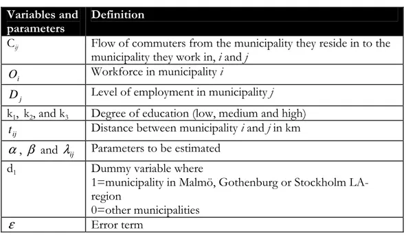
2 1 (Equation 4-6)Table 4-1 Definitions of the variables Variables and
parameters
Definition
Cij Flow of commuters from the municipality they reside in to the municipality they work in, i and j
i
O Workforce in municipality i
j
D Level of employment in municipality j
k1, k2, and k3 Degree of education (low, medium and high)
ij
t Distance between municipality i and j in km
α
, β and λij Parameters to be estimatedd1 Dummy variable where
1=municipality in Malmö, Gothenburg or Stockholm LA-region
0=other municipalities
ε
Error termSince variables O and D constitute the gravity-factor of the model, the expected relation between these and the dependent variable is as such: O, positive and D positive. Work-force O should have a positive coefficient because more competition in the municipality of origin creates a positive outflow of commuters. By the same token, D should have a posi-tive coefficient since more employment in the municipality of destination attracts more people to that municipality. The education variable k should according to the expectations increase with the degree of education. Distance should have a negative relation with the dependent variable because the longer the distance, the lower the probability that an indi-vidual would commute. If the dummy variable turns out to be significant in the regression, then the metropolitan areas are expected to have a strong effect on commuting.
4.2.1 Statistical errors
The reason to why there are only five parameters is to avoid the problem of multicollinear-ity, or just collinearity. The ideal scenario is when all the different X parameters contain unique information about the dependent variable Y which is not in any other of the X pa-rameters. When measuring the collinearity between two X parameters it is the correlation being measured. It is hard to get away from collinearity; it is very rare to see a case com-pletely without collinearity. When the X parameters are highly correlated it means that the two variables are containing much of the same information.
There are several ways of decreasing the problem of collinearity, and the most used routine is dropping the collinear parameter from the regression model. One can also change the sampling plan and also include elements from outside the range of collinearity.
4.3 Result
The regression model has been estimated with the ordinary least squares method (OLS). Table 4-2 shows the result of the following estimation equations (Equation 4-4, Equation 4-5 and Equation 4-6). ij ij k k j k i k ij
O
D
t
C
1=
ln
α
+
β
ln
1+
β
ln
1−
λ
1+
ε
ln
2 1 (Equation 4-4) ij ij k k j k i k ijO
D
t
C
2=
ln
α
+
β
ln
2+
β
ln
2−
λ
2+
ε
ln
1 2 (Equation 4-5) ij ij k k j k i k ijO
D
t
C
3=
ln
α
+
β
ln
3+
β
ln
3−
λ
3+
ε
ln
2 1 (Equation 4-6)All the parameters in Table 4-2 were statistically significant at α=0.05 except for employ-ment which is insignificant. The standard error, which is the square root of the variance, of the variables shows the difference between the estimated and true value of the parameter. The standard error is a very simple and often used measure of uncertainty in the value pre-dicted. The low numbers in the column mean that there is a small distance between the es-timated value and a true value which is just what one wants from the regression result. The coefficient column in Table 4-2 shows the estimates of the variables that have been standardised and have a variance of one. These values will tell us which of the independent variables that have a greater effect on the dependent variable. From the coefficient col-umns, one can see that—in general—the higher the education, the bigger the likelihood to start commuting. A one per cent change in the low-education category will give a 0.052 per cent change in the elasticity (elasticity since the variables are linearly logged) of total com-muters.
The regressions have also been tested for multicollinearity with the VIF-test (Variance Infla-tion Factor) which is a way of detecting the severity of the multicollinearity. As a rule of thumb one says that if the variable has a VIF-value of 10 or higher multicollinearity is a problem (Gujarati, 2003). None of the values reach above 1. In Table 4-2 all the VIF-values are around one and one can conclude that this regression does not suffer from any severe multicollinearity.
Then it is only the t-value column left. The t-value is a way of telling if the null hypothesis is true or not; the t-values were decided, in this case, being less than 5%, to be significant. Observable from these regressions, all the k variables’ t-value is significant at a 5 per cent level since the t-value for all k’s are larger than the (rule of thumb) value of 2 and should therefore be included in the regression model, and it also tells us that the null hypothesis cannot be rejected. This means that a high ratio of education in a municipality makes it more likely that the flow of commuters increases.
To measure the fit of the regression, the multiple coefficient of determination (R2) will be used. This “measures the proportion of the variation in the dependent variable that is ex-plained by the combination of the independent variables” (Aczel & Sounderpandian, p. 502, 2006). This means that R2 is measuring how good the modelfits the data. The values the R2 can take on lies between 0 and 1, where 0 means that the model is not showing a linear relation between the dependent and independent variables. One (1) is thus the per-fect fit and desired value. When R2 is one (1) the model used can explain all the variation in the Y variable (Aczel & Sounderpandian, 2006).
What one should know about the multiple coefficient of determination is that it may, as many other statistical measures, show the wrong result. The R2-value increases with the number increase of variables in the model. This is why there is also an adjusted R2 which will only increase if the new parameter actually improves the model. This is why the ad-justed measure of R2 is preferred over the original R2.
Table 4-2 Regression result of low education level as an independent variable Variable Coefficient Standard Error VIF-value t-value
Constant -2.406 0.027 - -88.915*
k1 0.052 0.003 1.474 15.414*
Employment 0.002 0.002 1.118 1.010
Distance -0.105 0.002 1.269 -48.023*
Workforce 1.153 0.002 1.067 626.668*
R2 = 0.835 Adjusted R2 = 0.835 No. of observations = 83515 *significant at α =0.05
Below, in Table 4-3 we find a 0.022, positive coefficient for the middle-education category. A one percent change in education will lead to a 2.2 percent change in the commuting of the middle educated people. Also here the standard errors are low, and so are the VIF-values. All the variables are significant at α =0.05 except for employment which is signifi-cant at α =0.1.
Table 4-3 Regression result of middle educational attainment level as an independent variable Variable Coefficient Standard Error VIF-value t-value
Constant -2.384 0.028 - -86.387*
k2 0.022 0.006 1.426 3.707*
Employment 0.005 0.002 1.138 -2.532**
Distance -0.093 0.002 1.159 -44.289*
Workforce 1.149 0.002 1.115 610.024*
R2 = 0.834 Adjusted R2 = 0.834 No. of observations = 83515 *significant at α =0.05 **significant at α =0.1
From the coefficient column in Table 4-4 one can see that the higher the share of educa-tion, the bigger the likelihood to start commuting since a one per cent change in the high education category will give a 0.124 per cent change in the elasticity of total commuters. Just as in the two above made regressions the regression with the higher level of education has a low value of the standard errors and low VIF-values. All the variables are significant at significant at α =0.05.
Table 4-4 Regression result of high education level as an independent variable
Variable Coefficient Standard Error VIF-value t-value
Constant -2.413 0.027 - -89.655*
k3 0.124 0.005 1.425 25.439*
Employment 0.007 0.002 1.106 3.741*
Distance -0.114 0.002 1.255 -52.584*
Workforce 1.156 0.002 1.050 634.864*
R2 = 0.836 Adjusted R2 = 0.836 No. of observations = 83515 significant at α =0.05
The null hypothesis used for the regressions is stated as follows:
H0: High education (k3) is significant for the outcome of the commuting decision HA: High education (k3) is not significant for the outcome of the commuting decision To see whether the error terms in the regression suffer from heteroscedasticity the White’s test has been conducted and the result from the test is given in Table 4-5. The p-value of the Obs*R-squared is 4051.911>0.05 which reveals that the error terms in the first regres-sion do not suffer from heteroscedasticity. Since the low level of education regresregres-sion did not suffer from heteroscedasticity further testing seems redundant.
Table 4-5 White's heteroscedasticity test for regression with low education White’s Heteroscedasticity Test
F-statistic Probability (F-stat.) Obs*R-squared Probability (Obs*R2)
532.2580 0.000 4051.911 0.000
In the second regression the test is made to see if the LA-regions’ size matters when the individual is deciding to commute or not. The result from this regression is to be found in Table 4-6. A new equation with a dummy variable was constructed for this, as seen below in equation 4-7. A new hypothesis is also seen below.
ij ij k k j k i k ij
O
D
t
d
C
=
α
+
β
1+
β
2−
λ
+
1+
ε
1 1 1 1ln
ln
ln
ln
(Equation 4-7)H0: More densely populated regions experience more commuting
HA: More densely populated regions do not experience more commuting
Table 4-6 Regression result of densely populated regions as a dummy variable Variable Coefficient Standard Error VIF-value t-value
Constant -1.096 0.026 - -72.936*
Employment -0.007 0.002 1.008 -4.002*
Distance -0.85 0.002 1.016 -45.690*
Workforce 1.083 0.002 1.174 588.131*
d1 0.370 0.004 1.169 92.306*
R2 = 0.850 Adjusted R2 = 0.850 No. of observations = 83515 significant at α =0.05
The d1 variable represents the dummy for people living in the three largest (population-wise) LA-regions. Clearly, the dummy for the three largest cities is significant (92.306>2) and interestingly, the coefficient is positive. The positive 0.370 coefficient shows an in-creased commuting into the metropolitan areas of Gothenburg, Stockholm and Malmö. The Variable Inflation Factor-values show no sign of high multicollinearity since all values are under the rule-of-thumb number of 10.
5 Analysis
This thesis had the purpose of analysing the commuter flows in Sweden. Is there a differ-ence in the commuting patterns for those who live in urban regions, and furthermore does the level of education influence the commuting flow? This section will analyse the results from Section 4.3 with the help of the theories mentioned in Chapter 2.
Commuting can only exist if the benefits (utility), like a higher wage, outweigh the negative effects, the costs of commuting. Clearly, based on the beta-coefficients from the first re-gression Table, education is very determining in how people commute. A significant coeffi-cient of 0.124 for k3 shows a positive relation between education and the number of people commuting. Furthermore, there is strong pattern of increasing commuting with increased education. Above stated theories, among others Glaeser’s (1994), indicate this positive rela-tion between higher educarela-tion and increased number of commuters, and this the regression confirms. Education as an important factor determining overall commuting seems to be contingent on the level of education with a straightforward positive relation, that is, more education yields a higher chance of people commuting. Commuting can be seen as a way for the individual to increase the value of his/her own human capital since the individual is commuting to a job with a higher wage or even a better job.
The last interval, the regression variable k3, is the highest educated class. This class is the one most likely to look for a higher paying job and eventually finding it because of mostly two factors. These two factors are i) they have the highest educational attainment and will therefore more likely be aware of the job-offerings at other locations within or without their own LA-region and with that knowledge ii) they will more likely start to commute to work because finding and getting hired at a workplace better suited for their particular set of human capital also further rewards their already higher educational attainment through the spillover effects most likely to be present in the workplace environment. The environ-ment of a better suited workplace better promotes human capital with educational spill-overs and more likely offsets the incurred cost of commuting than would it for a lesser educated individual.
The small coefficient for the other education classes may be partly explained by the type of menial task jobs which are usually associated with this level of education such as store clerk, custodian/caretaker and assembly line worker. These types of work are non-professional in nature and there exists little differentiation in wages between LA-regions. This makes it less probable indeed for people with lower educational attainment to com-mute.
For the higher education levels, there is a clearer link between increased education and in-creased commuting as evident by the coefficients and in line with initial expectations. Higher wages for these levels are in line with the core model, where higher levels of educa-tion are directly correlated with higher paying wages, which are located in bigger agglom-erations (cities).
As expected from the regression model, the distance between the communities should be negatively related to the dependent variable of total commuting. From the regressions, one can see that this assumption is confirmed with the distance’s significant negative
beta-coefficient value, which would imply that for every unit increase in km the elasticity of total commuting will decrease by 8.5 per cent (in the dummy regression).
Employment is, according to both the regression results and from commuting theory, posi-tively correlated with the dependent variable of total commuters and implies that if the employment in one municipality is increasing the need to commute is increasing since more people look for work outside the municipality. In this case a one unit change in employ-ment will result in an approximate increase in elasticity of total commuting with 0.124 per cent in the high education category.
Workforce is positively correlated with the dependent variable and will increase with it. When there is a one unit increase in the workforce of a municipality the people will start to commute to other (larger) places nearby since there are now more competitors on the local labour market. The regression results show a positive change in the elasticity of the de-pendent variable when there is a positive change in the workforce.
The results from the regression regarding employment and workforce, both being posi-tively correlated to total commuters, are of course as expected since they are both measures of the gravitational force between municipalities in a sense.
In the regression with densely populated regions as a dummy variable there is an analysis of the significance of the most densely populated areas. The positive sign for the dummy’s coefficient is true to macroeconomic theory as stated before: human capital promotes geo-graphical mobility, and so people commute to cities. The larger labour markets in the mu-nicipalities of the three largest Swedish cities (Malmö, Gothenburg and Stockholm) should incite commuting from outlying and surrounding municipalities, creating ever larger (area-wise) LA-regions. This is supported by the gravity model since it is derived from both scale- and distance impacts, which supports the theory of attraction of people towards lar-ger cities, and also that the further away something is, the smaller is the interaction between the two municipalities. Since commuting is on the increase and people are more willing to be geographically mobile, it allows companies to agglomerate easier and benefit from economies of scale since the common man is not that strange anymore to the idea of commuting.
Companies strongly dependent on human capital more willingly accept that the employee is not living in an area close to the company. This can be due to the fact that the company really needs this knowledge. This fact then makes this particular type of job more immune to the effects predicted by distance friction theory; even when distances (whether measured in time or km) are relatively long, the acquired utility derived from commuting will often enough exceed the costs incurred from “going that extra mile”.
The R2 in all the regressions above is around 0.8, which is a fairly good value. Since there is no decided value of what is “good” and what is “bad” one has to “weigh” the resulting value against the rest of the regression.
The R2-value that was obtained in the education-regressions is in itself a good value but could be somewhat high for so few variables. One would expect there to be many other factors that would influence the commuting patterns and the choice of commuting other than just the degree of education, such as strong bonds with your family.
6 Conclusion
It is hard to get away from the fact that some municipalities are larger than others and more densely populated, meaning the result could be biased. A lot of mid- to high-level LA-regions (size-wise) are not represented with a dummy in the regression, even though there are still several tiers of LA-regions whose size-related influence on commuting it would be interesting to investigate. The quality of the thesis suffers because of this fact. Concluding from the results of the distance: it has a significant impact on the individual and his/her choice to commute. When the distance increases the willingness to commute is decreasing and when the distance decreases the willingness to commute is increasing. As a policy implication and also a suggestion for further studies, negative externalities and the effect of increased commuting on the environment could be taken into consideration. Considering the ongoing debate on global warming and man’s influence thereon, conjec-ture pertaining to this and associated policy implications should prove interesting to ex-plore. Further policy implications include infrastructural improvements (which are in Swe-den most often controlled by governmental decision makers), helping to lower commuting costs and easing the movement of people to better clear labour markets and thereby pro-moting growth.
After reading a lot on the subject of commuting one can conclude that there have not been done any Swedish studies on the effect of commuting on income. This is a very interesting subject since it shows how the incentives of the individual’s economy on commuting and migration work. As well as this study can be developed even more, the individual’s partner and possible family and how these factors affect the individual’s choice to commute can be taken into consideration. This kind of study would also benefit further from comparative data, e.g., cross-sectional data with an expanded time-frame, in effect, this could be done using data from separate years, comparing the result for both years.
References
Aczel A. D., & Sounderpandian J. (2006). Complete Business Statistics, (6th ed.). New York: McGraw-Hill/Irwin.
Alonso W. (1964). Location and land use: toward a general theory of land rent. Cambridge: Harvard University Press.
Anas, A. (1983). Discrete choice theory, information theory and multinominal logit and gravity models, Transport. Res. vol 17B(1), 13-23.
Bade R., & Parkin M. (2004). Foundations of Microeconomics (2nd ed.). USA: Pearson Addison Wesley.
Becker S., G., Murphy M. K., & Tamura R. (1990). Human Capital, Fertility, and Economic Growt, The Journal of Political Economy vol 98(5), 12-37.
Bergstrand J.H. (1985). The Gravity Equation in International Trade: Some Microeco-nomic Foundations and Empirical Evidence, The Review of EcoMicroeco-nomics and Statis-tics, vol 67(3), 474-481.
Borjas G. J. (2005). Labor economics, (3rd ed.). Boston: McGraw-Hill.
Brakman S., Garretsen H., & Marrewijk van C. (2001). An introduction to geographical economics: trade, location and growth. Cambridge: Cambridge University Press
Eliasson K., Lindgren U., & Westerlund O. (2003). Geographical labour mobility: migra-tion or commuting, Regional Studies vol 37(8), 827-837.
Eliasson K, Westerlund O., & Åström J. (2007). Flyttning och pendling i Sverige, Statens Of-fentliga Utredningar vol 2007(35).
Fujita M., & Thisse J.F. (1996). Economics of agglomeration, Journal of the Japanese and inter-national economies 10.
Glaeser L. (1994). Cities, Information and Economic Growth, Cityscape: A Journal of Policy Development and Research vol 1(1), 9-47.
Gujarati N. D. (2003). Basic Econometrics (4th ed.). Boston: McGraw-Hill.
Hamilton B. W. (1982). Wasteful commuting, The Journal of Political Economy vol 90(5), 1035-1053.
Haynes K. E., & Fotheringham S. A. (1984). Gravity and spatial interaction models. Beverly Hills: Sage.
Johansson B., Klaesson J., & Olsson M. (2002). Time distances and labour market integra-tion, Paper in Regional Science vol 81(3), 305-327.
Johansson B., Klaesson J., & Olsson M. (2003). Commuters’ non-linear response to time distances, Journal of Geogrphical Systems vol 5(3), 315-329.
Lindgren U., Eliasson K, & Westerlund O. (2002). Flytta eller pendla? In G. Malmberg (Ed.), Befolkningen spelar roll! (p. 61-75) Umeå: GERUM – kulturgeografi
Mincer, J. (1978). Family migration decisions, Journal of Political Economy vol 86, 749-773. Molho I. (1986). Theories of Migration: A review, Scottish Journal of Political Economy vol
33(4), 396-419.
Olsson M. (2002). Studies of commuting and labour market integration, PhD dissertation no.16, Nationalekonomiska Institutionen, Internationella handelshögskolan i Jönkö-ping.
Parr B. J. (2002). Missing Elements in the Analysis of Agglomeration Economies, Interna-tional Regional Science Review vol 25(2) 151-168
SCB (2005). Fokus på arbetsmarknad och utbildning.
Schultz W. T. (1961). Investment in human capital, The American Economic Review vol 51(1), 1-17.
Small K. A., & Song S. (1992). “Wasteful” commuting: A resolution, The Journal of Political Economy, Vol. 100(4), 888-889.
Varian R. H. (2003). Intermediate microeconomics: a modern approach (6th ed.). New York: Nor-ton.
Westerlund O. (2001). Arbetslöshet, arbetsmarknadspolitik och geografisk rörlighet, Eko-nomisk Debatt 2001 årg 29, nr 4, 263-272
Westerlund O., & Wyzan M. L. (1995). Household migration and the local public sector: evidence from Sweden, 1981-1984. Regional Studies 29(2), 145-157.
Appendices
Appendix 1
Appendix figure 1
Appendix 2 Appendix figure 2 k3 -1,00 -1,50 -2,00 -2,50 -3,00 12,00000 10,00000 8,00000 6,00000 4,00000 2,00000 0,00000 to tc o m m u te r R Sq Linear = 0,164 k3 Appendix figure 3 k2 -1,20 -1,40 -1,60 -1,80 -2,00 -2,20 12,00000 10,00000 8,00000 6,00000 4,00000 2,00000 0,00000 to tc o m m u te r R Sq Linear = 0,141 k2
Appendix figure 4 k1 -1,50 -2,00 -2,50 -3,00 -3,50 -4,00 12,00000 10,00000 8,00000 6,00000 4,00000 2,00000 0,00000 to tc o m m u te r R Sq Linear = 0,008 k1
Appendix 3
Appendix figure 5 Level of employment
13,00000 12,00000 11,00000 10,00000 9,00000 8,00000 7,00000 6,00000 12,00000 10,00000 8,00000 6,00000 4,00000 2,00000 0,00000 to tc o m m u te r R Sq Linear = 0,181 Level of employment
Appendix 4
Appendix figure 6 Incoming commuters
250000,00 200000,00 150000,00 100000,00 50000,00 0,00 800000,00 600000,00 400000,00 200000,00 0,00 p o p u la ti o n Incoming Commuters
Appendix figure 7 Outgoing commuters
100000,00 80000,00 60000,00 40000,00 20000,00 0,00 800000,00 600000,00 400000,00 200000,00 0,00 p o p u la ti o n Outgoing Commuters