Temperature distributions in cylinder-shaped bodies of asphalt mixes during and after conditioning in water-baths

(1)

Nr 258A « 1983 Statens vag- och trafikinstitut (VTI) « 581 01 Linkoping

ISSN 0347-6030 Swedish Road and Traffic Research Institute ® 8-581 01 Linkoping * Sweden

(2)

APRT

Nr 258A 0 1983

Statens véig- och trafikinstitut (VTI) 0 581 01 Linkoping

ISSN 0347-6030 Swedish Road and Traffic Research Institute 0 S-581 01 Linképing 0 Sweden

Temperature distributions

in cylinder-shaped bodies of

asphalt mixes during and after

conditioning in water-baths

(3)

(4)

PREFACE

This experiment work has been conducted at the

National Swedish Road and Traffic Research Institute in Linkoping. The evaluation of the test results as well as the writing of the report has been made at Dynapac in Karlskrona. I am greatly indebted to all those who made it possible for me to carry out this investigation. I would especially like to mention Bengt-Ake Hultqvist (M.Sc., Civ.Eng.),

Glenn Lindqvist (Eng) and Anders Crbom (B.Sc.) plus

all the research engineers at the Institute for

their assistance in setting up the equipement and in helping me with the measurements.

Anders Bjorklund

(M.Sc., Civ.Eng.)

(5)

(6)

C O N T E N T S ABSTRACT REFERAT SUMMARY SAMMANFATTNING 1. INTRODUCTION

2. PURPOSE AND PLANNING

3. BITUMEN AND MINERAL AGGREGATES

.1 Thermal properties of various consti tuents according to the literature and previous research by others

.11 Heat capacity .111 Bitumen .1l2 Mineral aggregates .113 Rubber .114 Asphalt mixes .12 Thermal conductivity .121 Bitumen .122 Mineral aggregates .123 Rubber .124 Asphalt mixes

.2 Choice of mix designs .21 Selection of bitumen

.22 Selection of mineral aggregates .23 Selection of mix compositions

4. THE OUTLINES OF THE TEST PROGRAM

.1 The influence of the specimen size

VTI REPORT 258 A Page II III VII C D C D \ I \ I \ I \ I O \ O \ O \ U 1 U 1 U 1 ®4 > \0

(7)

.2 The The The

influence of the measuring point influence of the voids in the mix influence of mix composition

5. THE TEMPERATURE MEASUREMENTS

.1 The equipment used The heating period .3 The cooling process

6. RESULTS

.1 Evaluation of the results .11 The heating period

.111 The influence of the specimen size and the measuring point location

.112 The influence of the voids in the mix .113 The influence of mix composition

.12 The cooling process

.121 The influence of the specimen size and the location of the measuring point .122 The influence of the voids in the mix .123 The influence of mix composition

7. SOME COMPARISONS BY THE AID OF THE

VALUES AND RELATIONSHIPS LISTED IN SECTION 3.1 8. REFERENCES 9. LIST OF APPENDICES VTI REPORT 258 A / 10 11 11 16 16 17 17 17 17 19 19 30 3O 3O 3O 41 43 44

(8)

Temperature distributions in cylinder shaped bodies of asphalt mixes during and after conditioning in water baths

by Anders Bjorklund, M.Sc., Civ. Eng.

National Swedish Road and Traffic Research Institute

S 58l 01 LINKOPING

Sweden

ABSTRACT

The behaviour of asphalt pavements under traffic loading and certain types of maintenance activities, such as heating and compaction, are greatly affected by the temperature distributions involved. In the search for appropriate temperature dependent

constitutive relations between stresses and strains in the different cases, some further knowledge is required. This applies, for instance, to the thermal properties of hot mixes. It is also of importance to see to what extent analytically based methods of temperature determination can be used. The purpose

of the present report has been to gain further

insight into these questions. For practical reasons the studies have been made on cylinder shaped

laboratory manufactured specimens of different sizes and compositions during and after conditioning in water baths. The temperatures have been monitored at the boundary as well as at the centre. The results obtained during the heating period corresponded closely to theory. This is true provided that

appropriate values of the thermal diffusivity of the samples of different composition were used. During cooling, the agreement with theory weakened. This was expected due to simplifying assumptions in the

theory. However, good agreement was obtained during the first 15 minutes.

(9)

II

Temperaturfordelningar i cylinderformade provkroppar av asfaltmassor under och efter konditionering i vattenbad.

8-581 01 LINKoPING

Sweden

REFERAT

Asfaltbelaggningars beteende under inverkan av trafik-last samt vissa typer av underhéllsétgarder sasom heating och packning paverkas starkt av forekommande temperaturfordelningar. I sokandet efter lampliga temperaturberoende konstitutiva samband mellan span-ningar och tojspan-ningar 1 de skilda fallen behovs en del ytterligare kunskap. Detta galler t ex de termi ska egenskaperna hos asfaltmassor. Det a: ocksa angelaget att klarlagga i vilken utstrackning analytiska berakningsmetoder for temperaturfordel ning kan anvandas. Avsikten med denna rapport har varit att fa ytterligare insikter i dessa fragor.

Studierna har av praktiska skal gjorts pa cylindriska, laboratoriepackade asfaltprovkroppar av olika stor lekar och sammansattningar under och efter uppvarm-ning i vattenbad. Temperaturerna har registrerats saval vid kanten som i centrum av proven. Resultaten som erhéllits under uppvarmningen har stamt val

med de beraknade. En forutsattning ar da att lampliga varden pa varmediffusiviteten anvants for de olika sammansattningarna. Nar det galler avsvalningen har overensstammelsen blivit samre. Detta var vantat pa grund av de forenklade antagan den som legat till grund for den teoretiska berak-ningen. God samstammighet har emellertid uppnatts

under de forsta 15 minuterna.

(10)

III

Temperature distributions in cylinder-shaped bodies of asphalt mixes during and after conditioning in water baths

8-581 01 LINKoPING

Sweden

SUMMARY

The behaviour of asphalt pavements during traffic loading is to a great extent affected by their

thermal properties. Hence the possibility of healing fatigue cracks as well as developing permanent

deformation may differ for different materials in the summer. Also maintenance activities by use of so called heating technique may show different

effectiveness depending on the thermal properties of the old pavement. The same can be said of the

available time of compaction of hot mixes of various compositions. To get a clearer and more realistic picture of any of these events, it is desirable to ascertain the prOper temperature distribution as a function of space and time. This is fairly easy when solely conduction of heat is taking place but more tricky when radiation is involved. However, even then (by use of Newton's law of cooling ) analytical solutions can be derived. In these solutions the thermal properties of the mix must be considered. The thermal properties of asphalt mixes and their constituents have already been determined by some investigators whose findings are shown in this

report. The uncertainty regarding the properties of the mix seems to be ruled by the voids in the

pavement and the mineral aggregate used.

(11)

IV

The purpose of this report has been to gain further insight into the thermal properties of hot mixes. At the same time it has been interesting to ascertain to what extent analytically based methods will

correspond to actual temperature measurements . For

practical reasons the studies were made on Marshall specimens of different sizes during and after condi-tioning in water-baths. This is also a question of certain interest since the effect of heating time of cores and Marshall specimens has been questioned. The investigation presented in this report was

divided into three steps, being

1. The influence of the specimen size 2. The influence of the voids in the mix 3. The influence of mix composition

The principal mix chosen for the test was a dense graded hard asphalt concrete with a maximum particle size of 16 mm. The mineral aggregate consisted of granite. The bitumen content was 6.1 per cent by weight of total mass. Temperature sensors were

installed at both the boundary and the center of the Marshall specimens. The radii of these samples

were-7.5 and 5-cm and the heights 2.5, 3.75 and 6.35 cm. All combinations were tested in step No. 1.

In step No. 2 the normal mix was compaCted with five and ninetyfive blows respectively on each side. This scheme produced a variation of voids from two to nine per cent in the samples of normal size used. Step No. 3 included some changes in the normal mineral aggregate composition.

(12)

In one test 20 per cent by weight of the coarsest fraction was replaced by quartzite. In another

rubber granules from scrapped tyres substituted some of the fine material in the range of 2-4-mm.

Moreover, a Gussasphalt taken from a work site was

included for comparison. In all cases, three samples of each composition were tested.

The results obtained during the heating period were in good agreement with theory. The deviations were greatest at the boundary of the smallest specimens. However, readings from the recorder were difficult

to make in these cases. A thermal diffusivity of l.03-lO"6 m2/s was found to be appropriate for the standard mix compacted to air voids of around three per cent. The corresponding value of the samples

with nine per cent voids was O.86-lO"6 m2/s. When

twenty per cent granite was substituted with

quartzite, the value increased to 1.29-10 6m2/s. The

samples with rubber granules included had a

diffusivity of 0.89-10 6. Most of this deviation was

due to high voids (around seven per cent) in the

samples. The Gussasphalt, finally, exhibited a

diffusivity of about 0.76-10'6 m2/s. All these

values seem to be in fairly good agreement with calculated values based upon the properties of the

constituents.

As far as cooling is concerned, the agreement with theory was poorer as time proceeded. This was

expected for reasons given above. However, good agreement was obtained during the first 15 minutes of the experiment. Then the results from specimens

of different sizes, voids and thermal diffusivity

could well be explained by the theoretical curves. This was valid for the measuring point at the

boundary as well as at the centre. The appropriate

(13)

VI

radiation coefficient found also seemed to be

justified from a theoretical point of View.

(14)

VII

Temperaturfordelningar i cylinderformade provkroppar av asfaltmassor under och efter konditionering i vattenbad.

8-581 01 LINKoPING

Sweden '

SAMMANFATTNING

Asfaltbelaggningars beteende under inverkan av trafik last péverkas starkt av deras termiska egenskaper. Saledes kan mojligheten till lakning av utmattnings

sprickor liksom framkallandet av kvarstaende deforma-tioner vara olika for skilda material under sommaren. Likasé kan underhéllsmetoder baserade pa uppvarmning ge olika effekt beroende pa de termiska egenskaperna hos den gamla belaggningen. Detsamma kan sagas om den disponibla tiden vid packning av asfaltmassor av olika sammansattningar. For att fa en klarare och mer realistisk uppfattning om nagon av dessa fall ar det onskvart att kunna uppskatta den verkliga temperaturfordelningen som funktion av lage och tid. Detta ar ganska enkelt nar endast varmeledning sker men besvarligare nar strélning forekommer. Till och med da, emellertid, (genom att anvanda Newton's avsvalningslag) kan analytiska losningar

harledas.

I dessa losningar maste de termiska egenskaperna

hos massan beaktas.

De termiska egenskaperna hos asfaltmassor och de i dessa ingéende delmaterialen har redan bestamts av nagra forskare vilkas resultat framgar av denna rapport. Osakerheten betraffande massans egenskaper tycks vara dikterad av halrummet i belaggningen och

av det anvanda stenmaterialet.

(15)

VIII

Avsikten med foreliggande undersokning har varit att fa ytterligare insikt i de termiska egenskaperna hos asfaltmassor. Samtidigt har det varit av intresse att utrona i vilken omfattning som analytiskt bestamda temperaturer motsvarar de verkligt uppmatta. Av

praktiska skal har studierna utforts pa Marshall provkroppar av olika storlekar under och efter kondi

tionering i vattenbad. Detta ar aven av visst intresse eftersom uppvarmningstidens langd for borrkarnor

och Marshallprovkroppar har diskuterats.

Undersokningen uppdelades i foljande tre steg l. Inflytandet av provstorleken

2. Inflytandet av hélrummet hos provet 3. Inflytandet av massasammansattningen

Standardsammansattningen som utvalts for forsoken var en tat, hard asfaltbetong med en maximal sten storlek pa 16 mm. Stenmaterialet bestod av granit. Bindemedelshalten var 6.1 viktsprocent av hela maSsan. Termistorer ingjots i saval kanten som i mitten pa Marshallproven. Radierna hos dessa prov var 5 och

7.5 cm och hojderna 2.5, 3.75 och 6.35 cm. Samtliga

kombinationer undersoktes i etapp ett.

I steg tvé packades standardmassan med fem reSp nittiofem slag pa varje sida. Detta orsakade en variation i

halrummet fran nio till tva volymprocent i de framstallda Marshallproven som var av normal storlek.

Etapp tre omfattade en del forandringar i den normala stenmaterialsammansattningen. I ett forsok ersattes 20 viktsprocent av den grovsta fraktionen med kvartsit. I ett annat utbyttes en del av finmaterialet i fraktionen

(16)

IX

2 till 4 mm mot gummigranulat ifran gamla bildack. Dessutom ingick en gjutasfalt, som tagits ifran en arbetsplats, for jamforelse.

Tre prov av varje variant avsags att undersokas.

Resultaten som erholls under uppvarmningen var 1 god overensstammelse med teorin. Avvikelserna var

storst i kanten av de minsta proven. Det var emeller

tid svart att avlasa skrivaren i dessa fall. En

termisk diffusivitet pa 1.03-10 6 m2/s befanns

passande for standardmassan packad till ett halrum kring tre procent. Motsvarande varde for proven

med sju procents halrum blev 0.86-10 6 m2/s. Nar

tjugo procent granit ersattes med kvartsit okade

vardet till 1.29-10-6 m2/s. Proven i vilka gummi

granulat ingick uppvisade en diffusivitet pa 0.89-10 6 m2/s. En del av denna avvikelse ifran standardprovets 1.03-10 6 beror dock sannolikt pa

det hogre halrummet i proven. Gjutasfalten, slutligen, erhall en diffusivitet pa omkring 0.76-10 6 m2/s.

Alla dessa varden tycktes stamma ganska val med

beraknade varden grundade pa massasammansattningarna och egenskaperna hos de ingaende delmaterialen.

Vad avsvalningen betraffar blev overensstammelsen

samre ju langre tiden fortskred. Detta var vantat

av de angivna skalen. God overensstammelse erholls emellertid under de forsta femton minuterna av experi mentet. Da kunde resultaten fran proven av olika

storlek, hélrum och sammansattningar val uttryckas med de teoretiskt harledda forloppen. Detta gallde matpunkten vid kanten lika val som den i mitten. Den framtagna strélningskoefficienten tycktes aven vara berattigad fran teoretisk synpunkt.

(17)

(18)

1 INTRODUCTION

Asphalt mixes can be described as visco elasto plastic materials which also are temperature

dependent. In fact, temperature changes often

greatly affect the rheological behaviour of a mix. This, in turn, can limit its use as a stable road construction material since under heavy traffic and during hot summer days the risk of getting ruts will increase. On the other hand, a maintenance activity of an existing road surface involving heating can be an attractive solution for bitumen bound materials in many cases. Moreover, the possibility of

compacting a bitumious material to a dense and durable course is greatly governed by its fluid state at excessively high temperatures.

Although all this is well known, some lack of know ledge appears to exist as to the thermal properties of the mix. It is true that some attempts have

already been made in this field (2), (3), (4) but

they are limited and mostly deal with the

constituents. Occasionally the question of proper heating times for Marshall specimens or cores is discussed. It is a matter of great importance in Marshall stability or creep testing. At colloqium 77

in Z rich, which primarily dealt with the

applicability of the static uniaxial creep test, this topic was brought up. The required time of

preheating related to the Marshall stability test is in the ASTM standard procedure stated to 30 to 40

minutes.

There have however been some changes in the Mix Design Methods For Hot Mix Asphalt Paving issued by the Asphalt Institute. The heating time is nov 30

and 40 minutes while the first edition (1) specified 20 to 30 minutes.

(19)

2 PURPOSE AND PLANNING

The scope of this paper was primarily to aquire addi tional information on the thermal properties of as phalt mixes. Another important purpose was to examine the agreement between the solution of the conventional heat conduction equation and the actual results of measurements. In this way the justification of ana

lytically based solutions of the heat conduction

equation can be assessed. This is important since such solutions of a multilayer road construction can be obtained fairly easily. It is also likely that temperature dependent constitutive equations for asphalt mixes can be formulated, which, in turn, Can faciliate the computation of realistic stresses and strains in a road resulting from different forces. For instance, the risk of getting permanent deforma

tions and/or cracks under heavy traffic can then be

ascertained.

However, the purpose of this investigations has been restricted to heating and cooling of cylinder shaped bodies of asphalt mixes during and after conditioning

in a water bath.

During the heating period the calculated temperature at any instant and any point can be expressed as

2 2 ' kCEE)t . kg' RI . {(-1)n _ 1}e L . l 0(Elr) @hgz;t): .1+ § 0 1 . nwz 8 El Sin m m l m H M S ,n. VTI REPORT 258 A

(20)

where 90 denotes the initial temperature difference

between the water bath and the specimen and 90(r,z,t)/GO the portion thereof developed at radius r and depth

2 at time t. JO and J1 designate as usual the Bessel functions of the first kind of order zero and one respectively. Moreover the last sum is to be extended

over all of the positive zeros of J0( a)=0,a being

the radius of the specimen and L its height. k is the thermal diffusivity. If t is expressed in seconds

r, a, z and L in m k shall be expressed in m2/sec.

The derivation of this temperature distribution formule is given in App. 2.

As can be shown from the expression, master curves can be drawn in a diagram showing 9(r,z,t)/ O as a

function of kt/a2 which both are dimensionless, so

that different curves will be obtained only for various r/a, Z/L and L/a ratios.

The cooling process that follows when the specimen has been taken out of the water bath may be analysed in a similar way. However, we now aquire a more elabo-rate expression

-k .2t

gl -kv 2t

m m .J (E.a)Jo( .r) e sinv é-cosv (z - Ede A 9(T,Z,t)==§§g£(2 l 1 l l ) n 2 n 2

( .2+32){Jo( -a)}2_l ₁ v L + sinv L_n _D

n=1 i=1

Here the summations shall be extended over all of

the positive zeros of EJ (Ea) - aJo (58) =

C3respec-. vL vL _ VL . . .

t1vely if tan j§- - 2 -<x which is approx1mately

inversively proportional to the thermal conductivity

(21)

and expressed in m 1 is a measure of the radiation

during cooling. This relation can of course also be shown in a diagram showing 9(r,z,t)/eO as a function

of kt/a2. However, different curves will then be

obtained for various r/a and z/L ratios and different magnitudes of d, a and L.

Primarily in order to verify these relationships and also to find out if and how different mixes with assumed different thermal diffusivities could be

fitted into these graphs a test program was made,

which was divided into the following 3 steps: 1. The influence of the specimen size

2. The influence of the voids in the mix 3. The influence of mix composition

3 BITUMEN AND MINERAL AGGREGATES

3.l Thermal properties of various

constituents according to the literature and previous research by others.

3.ll Heat capacity. 3.lll Bitumen

The heat capacity of bitumen is dependent on temperature according to the relation

Cbit(T) = Co(l+BT)

Pell (2) suggests a CO value around 1.67 KJ/KGOC and

a 8 value around 5-10 4/0C but dependent on the type

of the bitumen. This gives the following table

(22)

Temp T

0

20

60

100

200 0c

Cbit(T)

1.67

1.68

1.70

1.72 1.77 KJ/KgOC

Cbit(T)

1.7 -

1.9

2.1 KJ/KgOC

The figures on the second line are taken from (4).

They correspond to a B-value of 2-10 3/0C. 3.112 Mineral aggregates

The heat capacity of the mineral aggregate (Cagg) is of the order 0.70-0.84 KJ/KgOC, varying with type.

3.113 Rubber

According to (5) the capacity ranges from 1.88 to

1.93 KJ/KGOC.

3.114 Asphalt mixes

According to (2) the heat capacity of asphalt mixes is suggested to depend on the values of the bitumen and the mineral aggregate in the following way

cmix = 0.01 [(lOO-x) obit + xcagg]

Where x is the per cent of weight of bitumen of

total mass.

(23)

3.12 Thermal conductivity.

3.121 Bitumen

To the conductivity of most types of bitumen is assigned a value around 0.150 W/mOC but varying slightly with

temperature according to the relation 1(T) = A0 (1 C2T),

(2), where C2 depends on the type of bitumen and amounts to about 10 4 per 0C. This means a variation

shown below

Temp T 0 " 20 1 60 100 0C

A(T) 0.153 0.150 0.144 0.138 W/mOC

Bossemeyer (3) gives the values 0.175 W/mOC for bitumen and 0.140 W/mOC for tar.

3.122 Mineral aggregates

According to Bossemeyer significant differences in thermal conductivity exist between various types of mineral aggregates and also in different directions.

Examples Granite 3.14 4.07 W/mOC Limestone 1.22 W/mOC Quartzite 5.75 W/mOC Quartzite 6.36 W/mOC Basalt 1.40 - 2.79 W/mOC VTI REPORT 258 A

(24)

For dry air at normal pressure the value varies in the following way

Temp T 0 50 100 200 0C

A(T) 0.024 0.028 0.031 0.037 W/mOC

3.123 Rubber

According to (5) the conductivity lies in the range

0.174 0.233 W/mOC.

3.124 Asphalt mixes

Pell (2) and Bossemeyer (3) state that such values

are missing. The voids very likely play an important role.

Saal (2) has given the following equation for the conductivity of a mix

Amix = Abit°kagg

where Bv is the volume fraction of bitumen. This could probably only be applied to well compacted

mixes. Bosemeyer (3) states

Amix= 0.58 W/mOC for gussasphalt and Amix= 1.28 2.68 W/mOC for ordinary mixes

3.2 Choice of mix designs

3.21 Selection of bitumen

The bitumen chosen for the test was a pen 80/100 straight run bitumen normally used in Sweden.

(25)

3.22 Selection of mineral aggregates

As shown above granite and quartzite are said to exhibit different thermal conductivity. They are also to some extent used in the most common hot-mix

in Sweden (HABl6T). Thus it was decided to use

granite and quartzite in the tests.

Rubber particles from scrapped tyres are to a small extent also being used in hot mixes today. Since their thermal properties greatly deviate from those of normal mineral aggregate, some mineral particles were replaced by rubber granules in one test.

3.23 Selection of mix compositions

A dense graded hard asphalt concrete with a maximum particle size of sixteen mm was chosen for the test. The bitumen content was set at 6.1 per cent by

weight of the total mass (pen 80/100). However, this value was slightly adjusted for the mix with rubber granules. The reason for this was that an equal amount of bitumen expressed in per cent of volume was required.

A mastic aSphalt (gussasphalt) was furthermore intended to be included. However, this mix originated from a working site with unknown

constituents. The interest in this mix was based on its alleged different rheological behaviour from normal asphalt concretes. Also, as mentioned in section 3.124, it is said to have a lower thermal conductivity than normal hot mixes.

(26)

4 THE OUTLINES OF THE TEST PROGRAM

4.1 The influence of the specimen size

A dense graded hard asphalt concrete with a maximum particle size of sixteen mm and composed of granite

was mixed. The bitumen content was 6.1 per cent by weight of the total mass (pen 80/100). By using the

Marshall compaction equipment specimens of the radius 7.5 cm and 5 cm were manufactured. The heights of the smaller ones were made 2.5 cm

(representing cores from thin pavements) and 6.35 cm (which is the nominal height of a Marshall

specimen). This gave L/a ratios of 0.5 and 1.25 respectively. Analogously the height 3.75 cm was chosen for the larger diameter. Also here a height of 6.35 cm was used on some samples.

4.2 The influence of the measuring point

Small holes (¢=4 mm) for calibrated thermistors were

premanufactured during compaction at a distance

r = 0.8a from the center as well as in the middle.

The depths were respectively L/3 and L/2.

4.3 The influence of the voids in the mix Generally the Marshall compaction was conducted with fifty blows on each side. However, with the standard

mix (HABl6T with granite), which also was used in

step 4.1, normal Marshall briquettes (a = 5 cm L =

6.35 cm) were produced some of them with five blows

and some of them with 95 blows on each side. The surface had to be sealed on the most open samples to prevent the penetration of water. Sealing was made by hot bitumen.

(27)

10

The purpose of this step was to get an indication how much the thermal diffusivity was affected by a certain increase of the voids in the sample.

4.4 The influence of mix composition As indicated above a difference in the thermal diffusivity or the k-value of some mixes can be compensated for by taking another measuring time t, so that the factor kt/a2 remains unchanged. In order to test this assumption some changes in the original recepie were made. Out of these changed mixes three normal Marshall specimens (a = 5 cm L = 6.35 cm)

were manufactured (2 times 50 blows). The new mixes

were the following:

1. The coarsest fraction in the mix 12 - 16 mm (around 20 per cent by weight of the total

aggregate) was replaced by quartzite, which was

expected to have a greater thermal diffusivity. 2. 6 per cent by volume of the aggregate between 2

and 4 mm in the original mix were substituted with an equal amount of rubber granules from scrapped tyres. Keeping the bitumen content in per cent by volume unchanged required raising the value from 6.1 to 6.3 percent by weight. This was due to the lower true specific gravity of rubber

(1.19 g/cm3). However, judging by experience the

mix was also expected to be more open due to the different mechanical properties of the rubber particles. The purpose of this step was still to find what effect the rubber particles would have on the thermal diffusivity (the k value) of the mix. It was expected to be lower.

(28)

ll

3. Mastic aSphalt (the german Gussasphalt) was tested. As already mentioned the sample originated from a working site and the

constituents, above all the mineral aggregate, might very well have deviated from the normal granite used in the other tests.

5 THE TEMPERATURE MEASUREMENTS

5.1 The equipment used

The same two thermistors were used in all the tests. The sensors were put in their holes and were

carefully filled and insulated by using fine sand and a pure hard bitumen (pen 80/100). Each sensor was connected to an Operational amplifier causing an oscillator with frequency dependent on temperature. This output was fed into a monostable multivibrator, which was followed by an amplifier and a XT

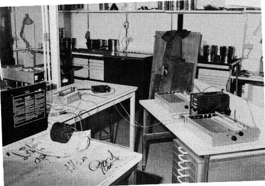
recorder. In this way the signal strength became a rather close function of the temperature. However, corrections were made at the final evaluation. The measuring system is described in Appendix 1 and the following pages show some photos of the practical

arrangement.

(29)

12 , m_n n

:s-

i'il-will" '

...

' V

;:;t

M

TIME:

Fig. 1 General views of the setup. The sample with the thermistors the waterbath and the

electronic circuit can be seen on the

left. The two recorders can be seen on the

right.

(30)

l3

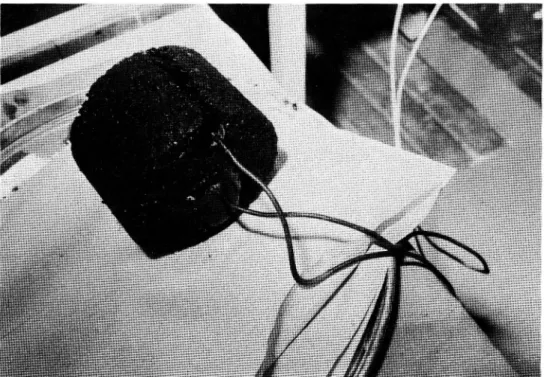
Fig. 2 A sample with the termistors installed. This being the position during the cooling period.

(31)

l4

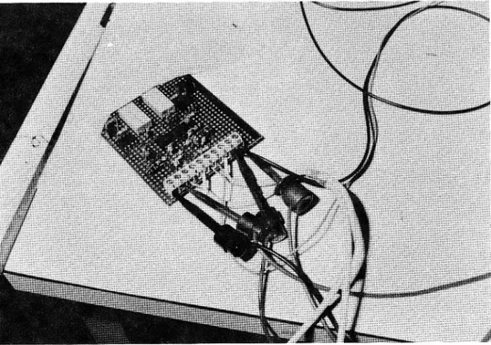
Fig. 3 The electronic circuit consisting of the

oscillators the monostable multivibrators

the low pass filters and the amplifiers.

(32)

15

' 4 One of the XT-recorders and the associated

voltage supply.

(33)

16

5.2 The heating period

The sample with the thermistors installed was connec-ted to the electronic circuit before it was placed

in the water bath. It had a constant temperature of

about 600C, the room temperature varying around 280C. The rise in temperature of both thermistors was

moni-tored by recorders. The specimen was taken out when further temperature rise was found negligable. For the normal Marshall specimen this was found to take place after 20 to 30 minutes.

After the tests these graphs were carefully read

1.25, 2.5, 5, 10, 15 and 20 minutes from the starting

time and to a certain extent corrected owing to some slight nonlinearity.

5.3 The cooling process

When the temperature in the sample had reached the constant ambient temperature the briquette was taken out of the water bath and placed on a table at some distance in order to monitor the cooling. The specimen was placed on its curved surface in order to limit

the influence of a practical support as far as possible. The readings on the recorders were followed conti

nuously until the temperature decrease of the mid point of the specimen was negligible. To a large extent this happened at a cooling time approximately five minutes longer than the corresponding heating period. However, the temperature by this time had

not yet gone down to room temperature. For evaluation

the temperatures at 5, 10, 15, 20 and 25 minutes

were read, corrected and expressed in fractions of

the initial temperature difference 90 between the sample (water bath) and the room temperature.

(34)

l7

6 RESULTS

6.1 Evaluation of the results

In appendix 2 and 3 theoretical solutions for the heating process and the subsequent cooling period are derived. These are based on very ideal

conditions. Especially the boundary conditions during cooling (the so called Newton's law) may be queried. The results from the theoretical analysis have been expressed as shown in section two. The numerical calculations are explained in appendix 4. The results from the practical measurements have been transformed to a e(r,z,t)/ O relation. An appropriate value of k has been determined in every

case, so that the measured values as well as

possible could be fitted into the diagrams having

kt/a2 as the independent variable.

6.11 The heating period

6.111 The influence of the specimen size and the measuring point location.

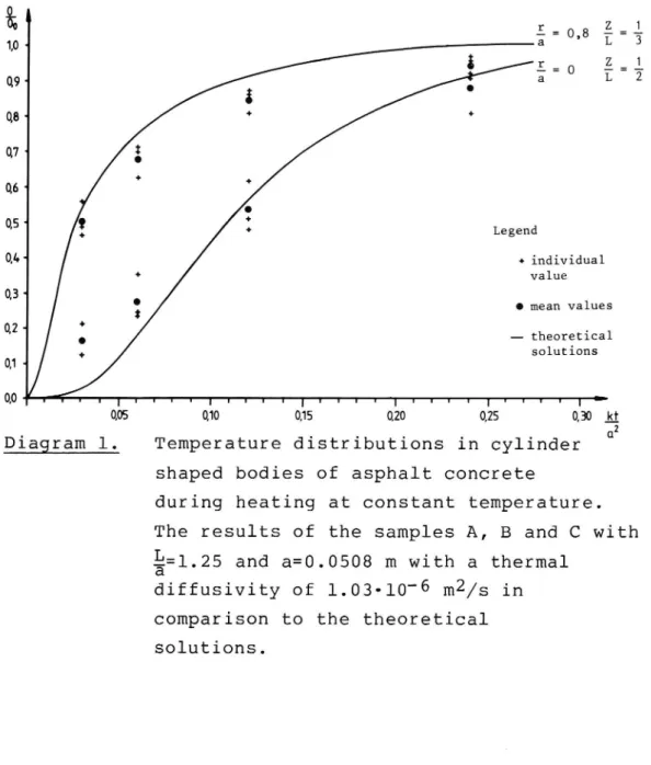
In diagram no. 1 the results from samples A, B and C are shown. These specimens have all a radius (a) of

0.0508 m and a height (L) of 0.0635 m. The best

correspondance with the theoretical values seems to

occur for a k-value around 1.03-10 6 m2/s. Then the

value of kt/a2 were 0.03, 0.06, 0.12 and 0.24

respectively at times t = 1.25, 2.5, 5 and 10

minutes resp. The agreement was fair at the boundary

as well as in the center.

The next diagram shows the results from the specimen D, E and F. The radius was 0.075 m and the height

(35)

18

0.0635 m. Since these samples were also manufactured

from the standard mix a k value of l.03-lO"6 mZ/s was used. As shown the results for t = 1.25, 2.5, 5, 10 and l5 min expressed as kt/a2 agree with the theore

tical results at the boundary as well as in the center. Diagram 3 shows the same results for the thinnest

samples (a = 0.0508 m; L = 0.0254 m). These samples were designated G, H, I. In this case the results deviated somewhat from the theory. A thermal diffu

sivity (k value) of 1.03-10-6 was adapted, since the

standard compositions were involved.

Finally, on diagram 4, the results from samples K, L

and M are shown. The same mix as earlier is being used and k is taken to be 1.03-10 6 m2/s. The radius was 0.075 m and the height 0.0375 m. Also on these comparatively thin samples the measured values differ slightly from those predicted. However, the agreement is better than for the G, H and I samples. In an

attempt to summarize the influence of the specimen size and measuring point it appears to be covered by the theoretical solution at least within the area investigated. The deviations are greatest at the boundary of the smallest specimens. However, reading of the XT recorder was very diffiCult in these cases. The appropriate thermal diffusivity of all

these-samples was found to amount to 1.03-10"6 m2/s. As can be seen in appendix 7 these samples were made out of the original mix and compacted by two times fifty blows in the standard equipment.

The resulting voids were all in the range 1 3 per cent by volume. With the aid of the relationships in section three thermal conductivities of the granite were calculated (see appendix 8). They were all found

(36)

19

to vary between 3.01 and 3.08 W/mOC, which close to the range previously mentioned.

6.112 The influence of the voids in the mix

The samples N, O and P were compacted with only two times five blows to normal Marshall specimens (a=0.058 m L=0.0635 m). Since they were made of the original mix, any differences in the k value ought to depend on variations in the voids. The measured values fitted the predicted values closely (see diagram 5) provided

that the k-value was put to 0.86-10 6m2/s. This was

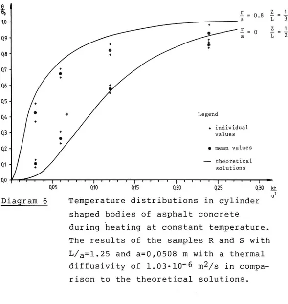
valid at the boundary as well as at the center. The voids of the samples were all around 7%.

Only two samples R and S of normal size were compacted by two times 95 blows. The results from those samples were all in accordance with the theory if the k-value 1.03-10 6 m2/s was used. The increase in density of these specimens was negligable. The results are shown on diagram no 6.

6.113 The influence of mix composition

In the specimens T, U and V of normal size and

compac-ted in the usual way (two times fifty blows) the

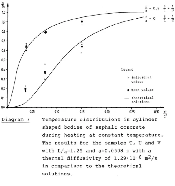
fraction 12-16 mm (20 percent by weight) consisted of quartzite. The mix recipe was otherwise unchanged. The results from these samples are shown on diagram no 7. From this diagram it is evident that a k-value

of 1.29-10 6 m2/s is most appropriate, since the

agreement at the boundary as well as at the center is very good.

(37)

20

As mentioned rubber granules were substituted for

granite in the fraction 2-4 mm in the original mix. The replacement was made on an equal volume basis. The briquettes from this mix were designated X, Y, Z. They were compacted according to the normal Marshall procedure. The resulting voids in the

samples amounted to around 8% by volume.

Hence the increase in bitumen content, expressed in per cent by weight and caused by the lower true speci fic gravity for the rubber, was not enough to reach the normal low void content. This was ascertained

from experience and can be explained by the compliance of the rubber particles. They oppose compaction.

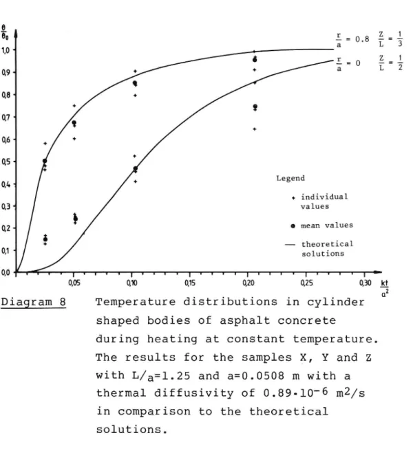
The best agreement with theory for these samples was

obtained using a k value of 0.89-10'6. This can readily be seen from diagram no 8. As shown (diagram no 5)

this is close to the results for the open samples of the original mix. As a result one may suppose that the presence of this amount of rubber particles does not lower the thermal diffusivity. However, in trying to compute the thermal diffusivity from the proper ties of the constituents, as described in section

3.1, one should have a lower k value, at least for dense specimens. One can thus say that the asphalt

rubber mix does not appear to be as sensitive to changes in the voids as the normal mix.

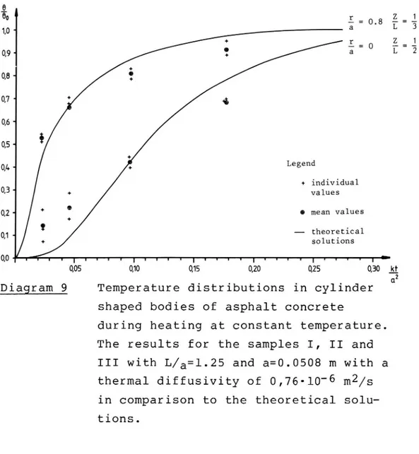
On diagram no 9 the results from samples I, II and III from the Gussasphalt are shown. Here the lowest

thermal diffusivity was reached, 0.76-10 6 m2/s,

although the voids was only around 2.5 per cent by volume. However, this is in fairly good agreement with section 3.124.

(38)

21

&lb

_r-

_E=l

1o« 3"m8 L 3 i r _ E = 1 Q9. 3'- O L 2 W W i 0' % QS Legend Q4. + individual value 03' 0 mean values QZ theoretical solutions 01-0,0 I I T I T I I I T T T I T T T T I I T T T I U T T T I ; 0,05 0,10 0,15 0,20 0,25 0, 30 _t

Diagram 1. Temperature distributions in cylinder shaped bodies of asphalt concrete

during heating at constant temperature. The results of the samples A, B and C with

g=1.25 and a=0.0508 m with a thermal

diffusivity of 1.03-10-6 m2/s in

comparison to the theoretical

solutions.

(39)

22 g6 l r Z 1 E- : 0 . 8 I = 3 10* E = 0 .E = 1 L _ 09 2 08 W 06* 05-Legend 04-+ individual 03 values I mean values 02-theoretical 01- solutions 0,0 I I I I l I I r I I I I I I l I I r I l I I I I I I I I I I : 0,05 0,10 0,15 0,20 0,25 0,30 151 2 . . . C1

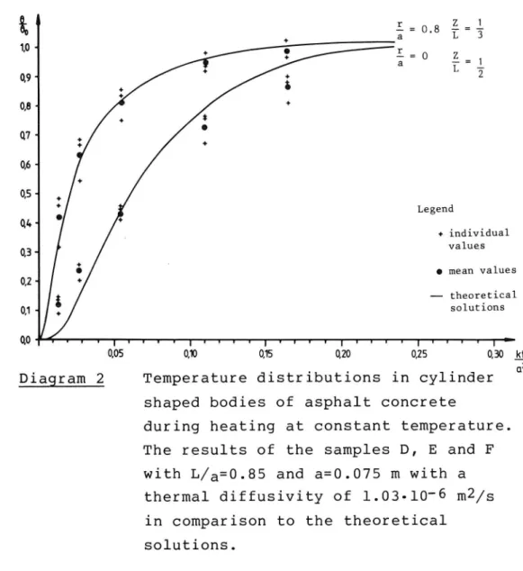
Diagram 2 Temperature distributions in cylinder shaped bodies of asphalt concrete

during heating at constant temperature. The results of the samples D, E and F

with L/a=0.85 and a=0.075 m with a thermal diffusivity of 1.03-10-6 m2/s

in comparison to the theoretical

solutions.

(40)

23

i

_mil _{;-d8 L}

r-

£=i

₃ 19 * 3.: 0 E.=.l % a L 2 w« + %i ₊ I_O

0.7 I

+

+ Q6* . QSJ + Le end Q44 g + individual Q3* values 02 0 mean values - theoretical OJ. solutions 0,0 I I I I I I I I I I I I I I l I I I I I I I I I : QOS 0J0 Q15 QZO Q25 k Diagram 3 N I -O ' 0

Temperature distributions in cylinder shaped bodies of asphalt concrete

during heating at constant temperature. The results for the samples G, H and I

with L/a=0.5 and a=0.0508 m with a

thermal diffusivity of 1.03-10-6 mZ/s

solutions.

(41)

6 24 r- .§=l W 2"m8 L 3 10 ₊ _{3.: 0} _%.=.% o 3 a 09- ₊ + 0,8 " + 9 o + + 07 06 + 2

05-i

04- Legend + individual QB values Q2 0 mean values 01 theoretical ' solutions 0,0 T I I T I I I I I I I f I I I 1 1 I i I T , l : 0,05 0,10 0,15 0,20 0,25 L1; 2 Diagram 4 (1

during heating at constant temperature.

The results for the samples K, L and M

with L/a=0.5 and a=0.075 m with a

thermal diffusivity of 1.03-10-6 mZ/s

solutions.

(42)

25

%"i r-= 0.8 Z -10 + a L i 3.: 0 E 0,9 + "' a L + W ₊ 0

mi

*

'0 0,6q 0 + %' 04 Legend + individual QB values Q2 0 mean values 01 theoretical solutions

0:0 '1 ['TTTI fVVIITr rvtr1TTTr.I;

0,05 0,10 0,15 0,20 0,25 0,30 LL

Diagram 5

02

during heating at constant temperature. The results for the samples N, O, P

with L/a=l.25 and a=0.0508 m with a

thermal diffusivity of 0.86-10-6 m2/s

solutions. VTI REPORT 258 A c o l d N l d

(43)

26

%

0 _{i = 0.8}

Z

_I 10 d + Z O E = 0 I 0,9 +₊ a 0 + 08 07 + o₊ %-05- + 04. Legend * individual 03 values Q2 9 mean values 01. theoretical ' solutions 0,0 I I I r I l 1 r r I I I I In. I l I I v I l I y l I T I I I T : 0,05 0,10 0,15 0,20 0,25 0,30 kf (1

Diagram 6 Temperature distributions in cylinder

shaped bodies of asphalt concrete

during heating at constant temperature. The results of the samples R and S with L/a=l.25 and a=0,0508 m with a thermal diffusivity of 1.03-10 6 m2/s in

compa-rison to the theoretical solutions.

(44)

27

%, n

r

_{-= 0.8} _-

Z

lO< a L

r _

z

09- 3"0 L 08 074 I %' 05 *-Q4 Legend 03 + individual ' values Q2 0 mean values Q1 theoretical solutions 0,0 t 1 v T I v 1 I v T t T r T 1 I I l t t r t T y y 1 1 I : 0,05 0,10 0,15 0,20 0,25 0,30 k_1 2 Cl

Diagram 7 Temperature distributions in cylinder shaped bodies of asphalt concrete

The results for the samples T, U and V

with L/a=l.25 and a=0.0508 m with a

thermal diffusivity of 1.29-10 6 m2/s in comparison to the theoretical

solutions. VTI REPORT 258 A N|-* wl -e

(45)

28

all 3:_a _0.8 E_L L0 3.: 0 % 094 a 08 Q. 07 1 0'6 d + 4' 05 0 Le end

041 g

+ individual 03 values 02 0 mean values - theoretical Q1. solutions 0'0 T I I r I V I t 1 I 1 I I I l I I U T 1 T I I 1 l I I I : 0,05 0,10 0,15 0,20 0,25 0,30 2

shaped bodies of asphalt concrete

during heating at constant temperature. The results for the samples X, Y and Z with L/a=l.25 and a=0.0508 m with a

thermal diffusivity of 0.89-10 6 m2/s

solutions.

(46)

29

all

r

Z

= 0.8 -10 a L + r - Z. Q9< Z"0 L 08-Q7. + 06%

05-

9

04- Legend + individual Q3. values QZ 0 mean values 01- theoretical I solutions 0,0 r f I t l l I I U l I U l u I y t j 1 I I , I r , , , I = 0,05 0,10 0,15 0,20 0,25 0,30 kf DN

Diagram 9 Temperature distributions in cylinder shaped bodies of asphalt conCrete

The results for the samples I, II and

III with L/a=l.25 and a=0.0508 m with a

thermal diffusivity of 0,76-10 6 m2/s

solu-tions. VTI REPORT 258 A un i-wl a

(47)

30

6.12 The cooling process

6.121 The influence of the specimen size and the location of the measuring point

On diagrams 10 - 13 the results of samples A, B, C

(10), D, E, F (11), G, H, I(12) and K, L, M (13) are shown. Only the position of the mean values have

been compared with the theoretical curves, since

diagrams with all values shown would have been diffi

cult to read. The scatter is, however, of the same order as during heating. The agreement between the mean values and the predicted ones seems to be fair only for comparatively short cooling times. The theo-retical curves have been calculated for an a value of 17. This d-value also seems to be of the right order although it is a little high when judging the temperature range involved (see appendix 4). In addi tion the influence of the measuring point appears to be rather well reflected by the theoretical curves. 6.122 The influence of the voids in the mix. The next diagram comprises the results from the open samples N, O and P. In this case a rather close agree-ment was obtained with the use of the corresponding k value of 0.86-10'6 mZ/s. This was valid irrespec-tively of the measuring points used. However, the scatter in the results is evident also here and only

the mean values have been used.

6.123 The influence of mix composition.

The poorest results seem to be those of the T, U and

V samples. Here it is difficult to see any significant difference between the results from the two measuring

(48)

31

points. For the asphalt rubber material a good agreement with the predicted curves exists when

judging by longer periods. However, the differences

between the boundary and the midpoint of the specimens are generally smaller than that of the

theoretical curves.

This is not the case for the Gussasphalt samples. The deviations from the estimated cooling curves

occur, however, as before after about 15 minutes

kt=O.25 .

(a2

>

(49)

32 0 _ L _ =

60 }

E-- 1.25 a 0.0508

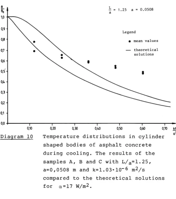
1,0 ' 0.9 Legend 0:8 ' _. 0 mean values 0.7 o theoretical 0_a solutions 0,6 + g , 3 05« ₈ 0,1. 0,3 -0,2 0,1 -0.0 1 l l I r I T 0,10 0,20 0,30 0,40 0,50 0,60 0,70

Diagram 10 Temperature distributions in cylinder shaped bodies of asphalt concrete during cooling. The results of the samples A, B and C with L/a=l.25,

a=0,0508 m and k=1.03-10-6 mZ/s

compared to the theoretical solutions

for a=l7 W/m2.

VTI REPORT 258 A

L

(50)

6 33

-1

_{60 l}

_{E.= 6-35 a = 0.075}

10 a 7.5 09- , Q8: . Legend Q7 . 0 mean values . O 06ql . . - theoretical. solutions 0 Q5 0 Q4- Q3-02~ Q1-QO 1 I I l l I I :: 0,10 0,20 0,30 0,40 0,50 0,60 0,70 5; 2 . . . (1

shaped bodies of asphalt concrete during cooling. The results of the samples D,

E and F with L/a=6§?§ , a=0.075 m and

k=l.O3-lO"6 m2/s compared to the theo

d=l7 W/m2.

retical solutions for

(51)

34 iJI 0.5 a = 0.0508 a_o m l r 1D Q9 Q8 Legend 0 mean values Q7 theoretical Q6 . solutions 0,5 - . 04-Q3- 0 0,2 « I . Q14 Q0 I I I I I ' I ' I' z; 010 020 030 040 050 060 070 _51 2 l I I I I I 0

Diagram 12 Temperature distributions,1n cylinder

shaped bodies of asphalt concrete during cooling. The results of the samples G, H and I with L/a=0.5,

a=0,0508 m and k=1.03-10-6 m2/s

compared to the theoretical solutions for d = 17 W/m2.

(52)

35 0.5 a = 0.075 #9 m l r Le end Q8+ g 0 mean values 07* _. O . theoretical solutions 0,6 « 0,5 « . 0,1. « . 0,3 -0,2 01 QO I 1 l l l I I 0,10 0,20 0,30 0,1. 0,50 0,60 0,70 f (1N

Diagram 13 Temperature distributions in cylinder shaped bodies of asphalt concrete during cooling. The results of the

samples K, L, M with L/a=0.5, a=0.075 m and k=l.03-lO"6 m2/s compared to the

theoretical solutions for d=l7 W/m2.

(53)

36 0

3 L-= 1 25 a = 0.0508

₃ 1,0

'-cpl

_o 08 ' Legend 0 g 0 mean values 0,7 4 theoretical 06 * . 0 solutions 0 0,5 " ~ . . 04-0 Q3 0,2 -ml 0'0 I l l l r l I ; 0,10 0.20 0,30 0,4 0,50 0,60 0,70 LL 2 u

Diagram 14 _{Temperature distributions in cylinder} shaped bodies of asphalt concrete during cooling. The results of the

samples N, O and P with L/a=l.25,

a=0.0508 m and k=O.86--lO"6 m2/s

for 0:17 W/m2.

(54)

37

9.1)

₀₀

3-: 1.25 a = 0.0508

_a 10 Q9 Legend Q8- 0 mean values 07 . . theoretical G solutions 0 06*1 G ° 0 o 05* 0 Q4- Q3-Q2d Q1 Q0 I I I I I I I 030 Q20 Q30 Q4 Q50 Q60 Q70

Diagram 15 Temperature distributions in cylinder shaped bodies of asphalt concrete during cooling. The results of the samples R and S with L/a=l.25,

a=0.0508 m and k=l.03-lO 6 m2/s

for d =17 W/m2.

VTI REPORT 258 A

's

di

(55)

38 .25 a = 0.0508 II u& 6

6'00

10* m l r 09 Legend 8-1 Q 0 0 mean values 07- I - theoretical solutions %- ₈ 05 04- 03-024 Q1~ 0,0 _l _T _I _I _l I _I : 0,10 020 0,30 0,40 0,50 0,60 0,70 31 2

shaped bodies of asphalt concrete during cooling. The results of the

samples T, U and V with L/a=l.25,

a=0.0508 m and k=1.29-10-6 m2/s

compared to the theoretical solutions for d=l7 W/m2.

(56)

39 0

53 a = 1.25 a = 0.0508

10 Q9 _Legend Q8 9 a mean values 0 Q7 theoretical solutions

06-

°

Q5 Q4* 8 Q3- Q2-Q1 0'0 I I I I I r I '1 Q10 Q20 030 Q40 Q50 Q60 Q70 _5i 2 0 Diagram 17 Temperature distributions in cylinder

shaped bodies of asphalt concrete during cooling. The results of the samples X, Y and Z with L/a=l.25,

a=0.0508 m and k=0.89-10-6 m2/s

for

VTI REPORT 258 A

(57)

4O

Q

E-= 1.25 a = 0.0508

0 a W 0'9 ' . Legend 0.8 0 mean values o 07 o . theoretical ' 0 ₀ solutions 0,6 o O o 05 ₀ 0,4 * 03 0,2 4 0,1 '1 W l I I I I I I 0,10 020 0,30 0L0 0,50 0,60 0,70

Diagram 18 Temperature distributions in cylinder shaped bodies of asphalt concrete during cooling. The results of the samples I, II and III with L/a=l.25,

a=0.0508 m and k=0.76-10-6 m2/s

compared to the theoretical solutions for a=l7 W/m2.

VTI REPORT 258 A

ml

:

(58)

41

7 SOME COMPARISONS BY THE AID OF THE VALUES

AND RELATIONSHIPS LISTED IN SECTION 3.1

The thermal diffusivity k(m2/s) is determined by the

relation k ' =_mix _{Cm X Ymix}. mlx _where A '_{le lS expressed}' in W/mOC, Cmix in J/KgOC and Ymix in Kg/m3. It is

thus possible to ascertain a mix value corresponding to each mix. If Cmix is calculated according to 3.114,

where Cbit is taken to 1700 J/KgOC (see 3.111) and

Cagg to 770 J/KgOC (see 3.112), the value 827 J/KgOC

will be achieved.

For the asphalt rubber composition the heat capacity of the rubber , CR, has also been taken into account on a per cent by weight basis. CR has been given the value 1900 J/KgOC in this calculation in accordance with 3.113. The mean bulk specific gravity of each group formed by the three samples has been used as the Ymix value.

As a result a Amix value has been obtained for each

group.-The relation in section 3.124 is of particular inte rest here. When using this it should be possible to

estimate the thermal conductivity (lagg) of the

aggre-gate in the composition based upon the volume rela tionships between the bitumen and the aggregate. If

lbit is taken to 0.15 W/mOC Aagg will be 3 -3.1 W/mOC

for the granite. However, this only seems to be valid for the dense graded compositions with voids around

% of volume. In the open samples (7%) N, O, P a value of 2.28 W/mOC was attained. Obviously correc-tions ought to be made in the formula mentioned. If

B . A 1 VV-BV

. . . V

the relation is changed to mix= X 3" X.V_air _bit _agg where lair designates the thermal conductivity for

(59)

42

air and VV the voids in the sample, better agreement

is obtained. If lair is taken to 0.028 W/mOC (see

3.122) the Aagg values willall be in the range 3.36 3.67 W/mOC for the granite used. The compound of granite and rubber also reaches a higher value 3.67 W/mOC, which might appear to be too high considering

the expected low thermal conductivity of the rubber granules. The corrected value for the quartzite compo sition amounts to 4.65 W/mOC. If this value is divi ded between granite and quartzite in the same manner as for the air the bitumen and the aggregate the value 12.25 W/mOC for quartzite is obtained. This is far too high considering the values listed in section

3.122. A more realistic value, 7.53 W/mOC, is attained

if the compound value is considered as a weighted average of the two constituents. The same conclusion can be drawn for the granite/rubber compound previously discussed. The mineral aggregate in the Gussasphalt material reaches 3.12 W/mOC (corrected) and 2.65 W/mOC (uncorrected). Some of these results appear in

appendix 8.

(60)

43

8 REFERENCES

1. Mix Design Methods For Hot-Mix Asphalt Paving. The ASphalt Institute First Edition April, 1956

Manual Series No. 2 fifth Printing, March 1959

2 Bituminous materials for flexible pavements University of Nottingham 1970

Lecture I: Strength and thermal properties of bitumen aggregate mixes.

3. Bitumen l/68

Die praktische Berechnung der Abk hlung bitumi noser Schichten.

H.R. Bossemeyer

4. H. Abraham, 1960

Asphalt and Allied Substances.

5. Miljons péverkan pa gummimaterial.

Gummitekniska foreningen STF & TU Kursverksamhet

(61)

44

LIST OF APPENDICES

Electronic circuit.

The temperature distribution in-a right circular cylinder as a function of time after it has been placed in the heated waterbath.

The temperature distribution in a right circular cylinder as a function of time after it has been removed from the waterbath.

The numerical calculations of the temperatures. Temperature variation with time during heating. Experimental results.

Temperature variation with time during cooling. Experimental results.

Bulk and true specific gravities for the speci-mens.

Calculated thermal conductivities for the mineral aggregate based on chapter 3 and the thermal

diffusivities found.

(62)

VTI REPORT 258 A OS CI LL ATOR HO NOST AB LE MU LT IV IBRA TO R + +

__

1

LO W PA SS FI LT ER J L AM PL IF IE R 050m t IS n

T

f

1/ 432 4 55 5 .I L

I I I

I

I I

|

I I

J

22 KI

_|

| | I

I I I I I

U 56 1.

KI 5,; I

I | I I I I I | I IR

C[

'o

n

I I I I I I I I

IN . 32 L OU T IT O XT RE CODE RI Electronic circuit Appendix 1 Page 1

(63)

RECORDER 0

@2414 OUT

THERMISTORS

B (In:

RECORDER OUT VTI REPORT 258 A Appendix 1 Page 2 *0 .»0 mo rO mO °O <0 -O 00 30

(64)

Appendix 2 Page 1

The temperature distribution in a right circular cylinder as a function of time after it has been placed in the heated waterbath

The solution is here derived by theuse of separation of

variable technique.

The governing equation of heat conduction expressed in cylindri cal coordinates is

2 2

ae _ k (a e + as + a e )

SE" arz r3r 322 ..(1)

Initial condition: 6(r,z,O) = 60 Oéréa

OézéL ...(2)

Boundary conditions: 9(a,z,t) = O nggL t > O .--(3)

9(r,O,t) = O Ogrga t > O ...(h)

t > O ...(5)

II _C) _{O l/\}fg /\ SD

e(r,L,t)'

Moreover i9(r,z,t)l < M where M is some positive constant i.e. l 6(r,z,t)l is limited.

Now let 6(r,z,t) = R(r)Z(z)T(t) and put it into (1) and divide both sides withlgR(r)Z(z)T(t).

(65)

Appendix 2 Page 2 Then I H I H T = B_.+ B__+ 2;. kT R rR z - ...(6)

As the left side is a function of t and the right side a

function of r and 2 both sides have to be constant Say ~12.

The minus sign is motivated since the solution must be limited.

kA2t

Hence T' = - kTA2 which gives T = Cle Where C1 is an

arbitrary constant.

The right hand of (6) gives

R" R' 2 Z" . .

-+ -= A - and again both Sides must be a constant,

R rR Z

- £2 say

Thus Z" + (12 52) Z = O or Z = CzelvZ + Cge_lvz

wherev2=AA{2.

Also rZR" + rR + rZEZR = O i.e. the Bessel equation with the solution R = CnJo( r) + CsYo (Er) where Cu and Cs are

arbitrary constants. However C5 = 0 here since R must be limited in the center.

One solution to (1) is thus ki2t iv

Z + Cse lvz) CuJo( r)

The boundary condition (3) now gives Jo (ia) = O (h) gives C3 = - C2 and

(5) elVL - e_l\)L = O i.e. v =-i

Hence\)andE;are the eigenvalues. The corresponding eigenfunc-tions multiplied with each other give the eigenfunction of the

system

_ . ~kA2t . n z _

6p C1 C2 Cu 21e Jo (air) Sin L

-(nu? 2

_

_Amie

k ~at - nwz

_L _{Sin -Ef-e}

kg. t

_{1 J0(Eir)}

(66)

Appendix 2 Page 3

The complete solution is obtained as the sum of the

eigen-functions or

2

6(r z t) § ( EA .e kgi tJo (gr) ) e k( L )t sin - mTZ_n1 ₁

The initial condition (2) now implies.

_ w m . nwz z w . n z = _

6(r,z,O) - g ( § AniJo (air) ) s1n if- § bns1n- E Go

2 L nwz 26 n

: ' - : 0 _. _

where bn L f ( 60) s1n L dz n {( 1) 1} 0

but bn = f AniJo (air) which according to Hankels inversion 1

theorem means that

a8; a

_

2 _ 2bn {yJ1 (3)}

Ani - a2 .2J1(a .) g₁ ₁ I anMEir) dr _ azg. J1 (air)0₁ ₁

he

_{° {(-1) 1}}

: nw

The complete solution to the problem is now T(r,z,t) = 60 + 6(r,z,t) =

2 -k .2t

6 {1 {(-1)n -1}e-k(EI:T-r-)t ' 3°59 l JD<Eir> sin

0 1 n" a 1 ii J1(Eia) L

Where the last sum should be extended over all of the positive

zeros of Jo( a) = O

(67)

Appendix 3

Page 1

The temperature distribution in a right circular cylinder as a function of time after it has been

removed from the heated waterbath

4

&

-_~.(_

The solution will be derived as before but with the following

changes:

Initial condition: 6 (r,z,O) = 60 Ogrga ...(8)

nggL

. . 36

Boundary conditions: SE-z d6(a,z,t) OézéL t>O ...(9)

36

SE-= d6(r,0,t) ogrga t>O ...(1o)

86

5E = de(r,L,t) Ogrga t>O ...(11)

(68)

Appendix 3 Page 2

As before one solution to the heat conduction equation is

- 2

-

_.

9p = C58 kl t(CselVZ + C78 lVZ) CeJo(Er) where v2 = A2 _ g2

which can also be expressed as

kA2t .

6p = C5e (Cgcosvz + ClosanZ) C8J0( r) 6p(r,z,t) = 6p(r,L-z,t) now implies that

CgCOSVZ + Closinvz = Cgcosv(L-z) + Closinv(L-z) =

= Cgcovacosvz + CgsinvLsinvz + ClosinvLcosvz Clocovasinvz

Identification gives

C9 = Cgcova + ClosinvL

C10 = CesinvL _ CloCOSvL - > which in turn means that

20 sin XL cos-XL

C =CgsinvL

:

9

2 2 = C tan 3g

10 1 + cova 2 vL 9 2

2cos 2 Then we will get

_k>\2t C9COSV(Z '%)

6 (r,z,t) = Cse . . CgJo( r) and

P _cos _~vL

2

36_{p =} _Cse-kA2t _. C9 .v sinv(z E-)₂ _{. 08J0(gr)}

32 _C

O, u

₂

39 (r L/2 t)

.

Note that

₃₂

E-

9 = o as 1t ought to be and that (10)

as well as (11) gives

vL _ . VL VL dL

vtan - § - a 1.e. -§-tan E- =

E-The roots of this last equation, the number of which is infinite, are all real. However, only the positive roots need

to be considered.

(69)

Appendix 3 Dana 3

d-vij

The corresponding eigenfunctions are given by L

cosvn(z '§) ¢n(z) = an

cos \m-L₂

To normalize these it is required that

2 L _{cos vn(}1 2 f C 9n 0

L.

-2) dz 1 2 z E. cos vn 2

However the left hand side of this equation is equal to

.L.

FL

1 + cos2vn(z 2 L 2cos2vn2 f 029n D ) _dz _{C 9n}2 1 _{L_Z 2Vn81n2vn(z 2)}}- 1 . L 2 .l 2cos vn2 2:0

1 l4-)}

2 C 9 2 1 1 L {L +-l- sin2v £ - O2v 2 l - sin2\)n2v

(

1 1 1 1 2cos2vn2

m.

V11 .L 2cos2vn2 2 L + C 9n .2 2 coszvn 2 sinan vn Hence ngn L+ (9) gives _ 2 _C (3 kk t Cgcosv(z

5 :19

cos 2 kx2t z acse Cgcosv(z VL ___.. 2 ie COS

5J1 (Ea) - aJo (Ea) = O

(70)

Appendix 3

Page 4

By superponation a more general solution 6 (r,z,t) can be obtained as 20t kg 1 cosvn(z -

E.

2

@(r,z,t) 22 AinJo( ir)e - C9 {3 an e COS * n=1 i=1

The initial condition (8) now gives ©(r,z,o) = Z Cn(r)¢n(z) = 60 n=1 where Ch(r) = z AinJo(gir) i=1 L Cn(r) = f 6(r,z,o)¢ (z)dz = o

L

= f e C cosvn(z 2) dz = e .C . 1 0 9n COS an O 9n vn

°

2

= 6 - 209 tan an 0 vn 2 a a

Now Ain = frCn(r)Jo(Eir)dr = f

°

0 i=1

2 2 a 0!, 2 = A .'nJ 2 ( 1 + EfY'){J0(EJ )}.a J 2 290C9n tan 2%L a 2 . _T'J .a A ' : Ej vn EA, 1(EJ ) nJ

a2( .2 +a2){Jo( .a)}2

_J

2

___:{sinvn(z

L.

2

an

2

which put into the expression for 6(r,z,t) gives

VTI REPORT 258 A

r<§AniJo(air))Jo(air)dr

)}

) kv 2t_n z=L z=O

(71)

Appendix 3

Page 5

-kg.2t kv 2t

l L 1 1

. L

-_ 890% m EiJ1( ia)Jo( ir)e Sinvn 2 cosvn(z 2)e

6(I',Z,t.)

2 2 2 .

+Cx' VnL + 8111an

n=1 i=1 ...(12)

where the summations are extended over all the positive zeros of EJ1( a) dJo(Ea) = O and

vL₂ _{tan 2}vL__g£₂ _{respectively.}.

(72)

Appendix 4

Page 1

The numerical calculations of the temperatures In order to achieve the graphs of the theoretical solutions the HP 97 calculator has been used. Above all it is the rootfinding program, which has been used to find the positive roots for 30(Ea) = O resp J1 (Ea) - dJO (Ea) = 0

vL vL dL

and if tan 7?- 2

These roots are all real and simple and for the first-relation also tabulated. In the two last ones you have to put in a proper value of . This is tricky, since it is gemperftgre dependent. A fair estimation seems to be Xmix (T1+T1T2+T1T2

temperature of the specimen (OK) and T2 an artificial

ambient temperature (OK). CS is 5.7-10 8 W/m2K4.

This will give an d value of about 8 W/m2 if Tl:

333.15 0K (600C) and T2 between 318,13 0K(450C) and 333.15 OK(6OOC). However, the corresponding roots

3 . . . .

#Ey where T1 is the initial

which determine the size of the sums in the expression for the temperatures will give too low values. By

trial and error an d-value of 17 W/m2 has been found

to be the most appropriate. The next page show the

corresponding positive roots and values of the Bessel functions for some arguments formed by some of them. Please also note that the different sizes of the specimens have been taken into account.

(73)

Appendix 4

Page 2

a = 0.0508 a = 0.075

a = 17 I

aa = 0.8636 _ r a0 = 1-275

The first positive zeros for aJ1( a) ano(£a) = 0

J0(gia ) La.

£.a Jo(O.8 ia) l

l J0(O°8gia) 1.3757u9u52 0.719339631 0.5T99h3861 n.1u15u0613 0.3h7180162 0.38h068282 7.193187032 0.077u20u91 0.295h3h151 10.29751173 0.1123h5801 0.2h779u2h7 13.h18090h7 0.212101516 0.195783553 19.67727095 0.1h58h5627 0.178678258 22.81681h20 0.0353hh821 0.13h5h5791 1.185115725 0.78759u033 0.678520870

h.0h7599h11 -0.3298h7657 -0.393577865

7.137032639 0.06303h8u5 0.297917809 10.25786268 0.120590677 0.2h8818596 13.38818h26 -0.2151u068u 0.217903066

19.6h96969u -0.1h285078h 0.178270800

22.90033390 0.03172778h 0.07531h201 a L a L a L

~§7-= 0.21250 for ET-= 0.31875 for § -= 2.53975 for

L = 0.025 L = 0.0375 L = 0.0635

The first positive zeros for v g tan 2% = 0-5

2-v L v L v L _£_ _3_ LE. 2 *__£L_____ 2 0.hh§271703 0.536275185 0.67h718517 3.2077h19v7 3.2396667h6 3.3035h6677 6.316813007 6.333h70735 6.3677h6290 9.hh7267hh5 9.h58h56183 9.h816h2382 12.58325653 12.5916795h 12.60915071 15.721h7898 15.72822661 15.7h223658 18.86082219 18.866hh939 18.878139h1 22.00080701 22.005632h9 22.01566030 25.1h119329 25.1h5h1682 25.15h19559 28.2818h739 28.28560239 VTI REPORT 258 A 28.293h08h5

(74)

Appendix 5

Page 1

Temperature variation with time during heating. Experimental results

Time 1.1/11. min 2.5 min 5 min 10 min (3.625 min. Estimated thermal

o o o 0 o 0 Ho 0 o 0 o e difquivgty (k Sample Tm C T0 C T C 5b T C 56 T C 56 T C 66 T C 6h value) m /s Am 60.0 25.0 32.5 0.21h 37.0 0.3h3 h6.0 0.600 56.0 .890 6 Bm 59.5 28.8 32.5 0.121 36.0 0.235 uh.0 0.h95 56.0 .886 1-03 ° 10 Cm 60.0 22.3 28.0 0.151 31.0 0.231 no.0 0.h67 52.5 .786 Mean 0.162 0.270 0.521 .85u ::::::i;:_ "" ________ _.==. Ak 60.0 25.0 hh.0 0.5h3 h9.0 0.686 5h.5 0.8h3 58.0 0.9u3

Bk

59.5 28.8 82.5 0.uh6 h7.5 0.609 53.0 0.788 56.0 0.886

1.03 . 10-6

Ck 60.0 27.6 h3.0 0.h75 50.0 0.691 55.0 0.8h6 57.5 .923 Mean 0.h88 0.662 0.826 .917 Dm 59.0 29.3 33.5 0.1h1 36.5 0.2h2 h2.3 0.h38 51.3 0.7h1 6 Em 61.0 27.5 30.h 0.087 3h.2 0.200 h2.3 0.uh2 52.2 0.737 1.03 - 10" Fm 60.0 2h.0 29.0 0.139 33.0 0.250 38.5 0.h03 h7.5 0.653 Mean 0.122 0.231 0.h28 .710 Dk 59.0 29.3 38.5 0.310 h5.0 0.529 51.0 0.731 56.0 .899 6 Ek 61.0i27.5 h2.5 0.hh8 h9.3 0.651 55.5 0.836 59.7 .961 1.03 - 10 Fk 60.0 2h.0 u1.0 0.h72 M8.0 0.667 53.5 0.819 57.0 .917 Mean 0.h10 0.616 0.795 .926 Gm 60.0 28.3 h8.0 0.621 53.0 0.779 56.8 0.899 59.7 .991 h1.0 0.u01 6 Hm 59.0 31.0 hh.0 0.h56 50.610.688 56.h 0.891 58.0 0.9u7 no.0 0.316 1.03 - 10 In 60.0 26.0 h8.0 9,6h7 53,0 0,79h 56.5 0.897 59.0 .971 h2.0 0.353 Mean 0.575 0.75M 0.896 .970 0.357 Gk 60.0 28.3 52.5 0.763 56.2 0.880 59.0 0.968 h7.2 0.596 6 HR 59.0 31.0 50.7 0.70M 55.5 0.875 57.h 0.9h3 h6.5 0.55M 1.03 ' 10 Jk 60.0 26.0 h8.5 0.662 5h.0 0.82M 58.0 0.9h1 39.5 0.397 Mean 0.710 0.860 0.951 0.516 Km 60.5 30.5 h3.0 0.u17 A8.0 0.583 53.7 0.773 58.2 .923 6 Lm 58.0 27.0 no.0 0.h19 h3.9 0.5h5 h9.8 0.735 55.3 .913 1.03 ° 10 Mm 60.0 27.0 M2.0 0.h55 h5.0 0.5h5 50.5 0.712 56.0 .879 58.0 0.939 Mean , J 0.h30 0.558 0.7h0 .915 VTI REPORT 258 A

(75)

Appendix 5

Page 2

Time 1.1/11 min 2.5 min 5 min 10 min 0.625 min. Estimated thermal

diffusivity'(k

e e 0 0 0

Sample TmOC T20 T80

55 TOC

-50 TOC

3}

Value) m /S

Kk 60.5 30.5 h7.2 0.557 5h.2 0.790 58.7 0.9h0 60.2 0.990

Lk 58.0 27.0 h3.8 0.5h2 50.0 .702 56.0 0.935 58.0 1.000 1.03 - 10 6

Mk 60.0 27.0 hh.5 0.530 50.5 0 712 55.0 0.8h8 58.0 0.939

Mean 0.5h3 0.7h8 0.908 0.976

Nm 59.5 28.5 28.5 0.016 30.0 0.0h8 38.5 0.323 50.0 0.717 55.5 0.871

Om 60.5 31.0 32.5 0.051 36.u 0.183 uh.7 0.h6u 53.7 0.769 57.5-O.898 0.86 - 10'6

Pm

60.0 25.0 31.0 0.171 35.0 0.286 hh.0 0.5h3 5h.3 0.837 57.0 0.91M i

Mean 0.079 0.172 0.hh3 0.77M 0.89M Nk 59.5 28.5 39.3 0.3h8 h5.7 0.555 51.5 0.7h2 56.0 0.887 0k 60.5 31.0 0.698 0.875 0.9h2 0,86 - 10 6 Pk 60.0 25.0 h7.0 0.629 51.5 0.757 55.0 0.857 58.0 0.9h3.58.5 0.957 Mean 0.558 0.729 0.8h7 0.938 =====:1F:===1:::=:::=__ ____ p -_ _ - - "-":=====

Rm

_{60.0 28.1 32.0 0.122 37.5 0.295 M5.h 0.5h2 5h.0 0.812}

_{1 O3 . 10 6}

Sm

61.2 30.0 32.8 0.090 37.0 0.22M M8.3 0.587 56.5§0.8u9

°

Mean

;0.106

0.260

0.565

0.831

=======t====ip==== = __==:1.= _______________ _.. Rk 5h.6 28.1 37.7 0.362 hu.7 0.626 h8.5 0.770 51.0.0.86u 1 03 10-6 Sk 61.2 30.0 hh.7 0.h71 51.3 0.683 56.0 0.833 60.0§0.962 ' Mean 0.h17 0.655 0.802 g0.913 Tm 59.0 32.0 38.0 0.222 hh.0 0.uuu 50.0 0.667 55.5 0.870 _6 Um 60.5 25.5 31.h 0.169 35.6 0.289 u5.0 0.557 56.h 0.883 129 ° 10 Vm 60.0 26.0 32.0 0.176 38.0 0.353 M8.0 0.6u7 56.0.0.882 Mean 0.189 0.362 0.62h 0.878 Tk 59.0 32.0 h9.6 0.652 53.0 0.778 55.2 0.859 56.5 0.907 Uk 60.5 25.5 u6.0 0.586 52.3 0.766 56.u 0.883 58.7 0.909 1,29 . 10 6 Vk 59.0 26.0 h7.0 0.636 51.5 0.773 55.5 0.89h 57.6 0.958 Mean L 0.625 0.772 0.879 0.938 P

VTI REPORT 258 A

(76)

Appendix 5

Page 3

Time 1.1/h min 2.5 5 min 10 min 0.625 min, Estimated thermal

diffusivity (k

Sample TmOC T00 T00

9. TOC

9_

9.

9 value)m /s

° 00 00 00 00 00 Xm 60.5 28.5 32.5 .125 35.5 0.219 h3.0 0.h53 51.5 0.719 6 Ym 61.0 28.0 33.3 .161 36.0 0.2h2 hh.9 0.512 55.5 0.833 0.89 1O Zm 60.0 26.0 31.0 .1u7 3h.5 0.250 39.5 0.397 h7.5 0.632 Mean .1hh 0.237 0.h5u 0.728 Xk 60.5 28.5 h3.5 .h69 h9.h 0.653 55.0 0.828 58.5 0.938

Yk

61.0 28.0 u6.7 0.567 52.2 0.733 57.2 0.885 59.8 0.96M

0.89 10-6

Zk 60.0 26.0 M1.3 .h50 M6.0 0.588 52.3 0.77M 56.2 0.888 Mean .h95 0.658 0.829 0.930 Im 60.0 29.2 33.5 .1h0 35.8 0.21M h1.0 0.383 50.0 0.675 55.2 0.8uh 6 11m 59.0 26.5 29.0 0.077 32.0 0.169 39.7 0.h06 h8.3 0.671 0.76 10

IIIm 60.0 2u.0 31.5 0.208 3h.0 0.278 39.5 0.931 u8.0 0.667 5u.0 0.833

Mean .1h2 0.220 0.h07 0.671 Ik 60.0 29.2 hh.7 .503 h9.0 0.6h3 5h.0 0.805 57.8 0.929 6