ACCURACY-AWARE STRUCTURED FILTER PRUNING FOR DEEP NEURAL NETWORKS
by
MARINA VILLALBA CARBALLO
B.S. Industrial Electronics and Automatic Control Engineering, Universitat Politècnica de Catalunya, 2019
A thesis submitted to the Graduate Faculty of the University of Colorado Colorado Springs
in partial fulfillment of the requirements for the degree of
Master of Science
Department of Electrical and Computer Engineering 2020
© 2020
MARINA VILLALBA CARBALLO ALL RIGHTS RESERVED
ii
This thesis for the Master of Science degree by Marina Villalba Carballo
has been approved for the
Department of Electrical and Computer Engineering by
Byeong Kil Lee, Chair
T.S. Kalkur
Darshika G. Perera
iii
Villalba Carballo, Marina (M.S., Electrical Engineering)
Accuracy-aware Structured Filter Pruning for Deep Neural Networks Thesis directed by Assistant Professor Byeong Kil Lee.
ABSTRACT
Deep neural networks (DNNs) have several technical issues on computational complexity, redundancy, and the parameter size – especially when applied in embedded devices. Among those issues, lots of parameters require high memory capacity which causes migration problem to embedded devices. Many pruning techniques are proposed to reduce the network size in deep neural networks, but there are still various issues that exist for applying pruning techniques to DNNs. In this paper, we propose a simple-yet-efficient scheme, accuracy-aware structured pruning based on the characterization of each convolutional layer. We investigate the accuracy and compression rate of individual layer with a fixed pruning ratio and re-order the pruning priority depending on the accuracy of each layer. To achieve a further compression rate, we also add quantization to the linear layers. Our results show that the order of the layers pruned does affect the final accuracy of the deep neural network. Based on our experiments, the pruned AlexNet and VGG16 models’ parameter size is compressed up to 47.28x and 35.21x with less than 1% accuracy drop with respect to the original model.
iv
ACKNOWLEDGEMENTS
First, I would like to thank Pete Balsells and the Balsells Foundation, the University of Colorado Colorado Springs and Generalitat de Catalunya for giving me the opportunity of pursuing the MSc in Electrical Engineering through the Balsells Graduate Fellowship. Thank you for helping me to achieve this experience in the United States. Also, thanks to my advisor, Dr. Byeong Kil Lee, for his continuous assessment and encouragement. Without his support this research work would not have been possible. Finally, I would like to thank my family and friends in Colorado and Barcelona. Thank you for your unconditional support, without you I would not have reached this point.
v
TABLE OF CONTENTS CHAPTER
I. INTRODUCTION ... 1
1.1 Project motivation ... 1
1.2 Purpose of the Study ... 2
1.3 Accuracy-aware Structured Filter Pruning Scheme ... 3
1.4 Thesis Outline ... 3
II. INTRODUCTION TO NEURAL NETWORKS AND COMPRESSION METHODS ... 5
2.1 Introduction to Deep Learning and Neural Networks Concepts ... 5
2.1.1 History ... 5
2.1.2 Differences between Machine Learning and Deep Learning ... 6
2.1.3 Artificial Neural Networks ... 6
2.2 Convolutional Neural Networks... 8
2.2.1 Convolution Layers ... 9
2.2.2 Rectified Linear Unit (ReLU) Layers ... 12
2.2.3 Pooling Layers ... 13
2.2.4 Fully Connected or Linear Layers ... 14
2.3 Compression Methods ... 14
2.3.1 Low-rank Factorization ... 15
2.3.2 Huffman Coding ... 16
vi
2.3.4 Quantization... 20
2.3.5 Design of smaller architectures ... 22
2.4 Transfer Learning ... 22
III. RELATED WORK ... 24
3.1 Network Pruning ... 24
3.2 Pruning and Quantization Combination ... 26
IV. GENERAL PRUNING SCHEME ... 28
4.1 Model training and Objective Selection ... 28
4.2 Pruning ... 29 4.2.1 Pruning Level ... 30 4.2.2 Pruning Criteria ... 30 4.2.3 Pruning Algorithm ... 32 4.3 Fine-tuning ... 33 V. PROPOSED METHOD ... 35 5.1 Filter Pruning... 36
5.2 Pruning Schedule Algorithm ... 38
5.3 Quantization ... 40
5.4 CNN Models ... 41
5.4.1 AlexNet ... 41
5.4.2 VGG16... 42
5.5 Programming Framework ... 43
vii
5.7 Preliminary Characterization of the Network ... 46
5.7.1 Experimental Setting ... 46
5.7.2 Layer characterization ... 47
5.7.3 Implications ... 50
5.7.4 Analysis - Problems encountered and potential solutions ... 52
5.8 Pruning Criteria: 𝓵𝟏 norm vs. 𝓵𝟐 norms ... 53
VI. EXPERIMENTAL RESULTS ... 56
6.1 Pruning AlexNet model trained with CIFAR-10 dataset ... 56
6.1.1 Dataset and Simulation Environment ... 56
6.1.2 Layer characterization ... 57
6.1.3 Results ... 58
6.2 Pruning AlexNet model trained with CIFAR-100 dataset ... 68
6.2.1 Dataset ... 68
6.2.2 Layer characterization ... 69
6.2.3 Results ... 69
6.3 Analysis and comparison of AlexNet results ... 71
6.4 Pruned VGG16 model trained with CIFAR-10 dataset ... 74
6.4.1 Layer characterization ... 74
6.4.2 Results ... 76
6.5 Pruned VGG16 model trained with CIFAR-100 dataset ... 80
6.5.1 Layer characterization ... 80
viii
6.6 Analysis and comparison of VGG16 results ... 84 VII. CONCLUSION AND FUTURE WORK ... 88 APPENDICES
A. FLOPs CALCULATION ... 96 1. Convolutional Layers ... 96 2.Fully Connected Layers ... 97
ix
LIST OF TABLES TABLE
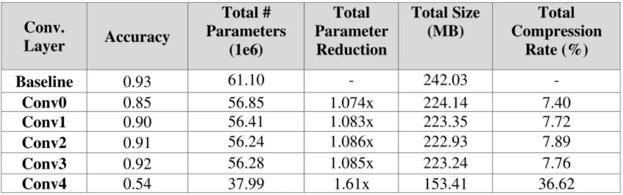
Table I. Results pruning each convolutional layer with Pr=0.5. ... 49
Table II. Output channels and number of parameters of the original pretrained AlexNet model layers. ... 49
Table III. Accuracy of the pruned model and accuracy drop with respect to the baseline according to the pruning order of the layers. ... 51
Table IV. Result comparison pruning all convolutional layers and excluding the last one. ... 52
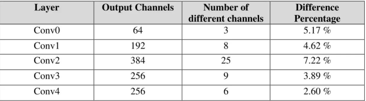
Table V. Difference in pruned channels when using ℓ1 and ℓ2 norms. ... 54
Table VI. Accuracy of the original pretrained AlexNet model trained with different number of epochs. ... 59
Table VII. AlexNet pruned model accuracy with different pruning order of the convolutional layers. ... 60
Table VIII. Accuracy results changing the pruning rate. ... 61
Table IX. Accuracy results using quantization. ... 64
Table X. Number of epochs and pruning rate used for Table XI experiments. ... 66
Table XI. Accuracy results for all the possible order combinations of convolutional layers in the AlexNet model. ... 66
Table XII. Results for compression and FLOPs reduction training the AlexNet model with CIFAR-10. ... 68
Table XIII. Accuracy of the original pretrained AlexNet model trained for 20 epochs with CIFAR-100. ... 70
Table XIV. Experiments using pruning and quantization in the AlexNet model trained with CIFAR-100. ... 71
x
Table XV. Results for compression and FLOPs reduction training the AlexNet model with CIFAR-100. ... 71 Table XVI. Order of convolutional layers and pruning rate for the AlexNet pruned model... 72 Table XVII. Results of the baseline original AlexNet model and results using the proposed Accuracy-Aware pruning method. ... 72 Table XVIII. Comparison of AlexNet results using CIFAR-10 with other state-of-the-art methods. ... 74 Table XIX. Accuracy of the original pretrained VGG16 model trained for 5 and 20 epochs with CIFAR-10. ... 77 Table XX. Experiments using pruning and quantization in the VGG16 model trained with CIFAR-10. ... 78 Table XXI. Results for compression and FLOPs reduction training the VGG16 model with CIFAR-10. ... 79 Table XXII. Accuracy of the original pretrained VGG16 model trained for 5 epochs with CIFAR-100. ... 82 Table XXIII. Experiments using pruning and quantization in the VGG16 model
trained with CIFAR-100. ... 83 Table XXIV. Results for compression and FLOPs reduction training the VGG16 model with CIFAR-100. ... 84 Table XXV. Order of convolutional layers and pruning rate for the VGG16 pruned model... 84 Table XXVI. Results of the baseline original AlexNet model and results using the Accuracy-Aware proposed pruning method. ... 85
xi
Table XXVII. Comparison of VGG16 results using CIFAR-10 with other state-of-the-art methods. ... 86 Table XXVIII. Comparison of VGG16 results using CIFAR-100 with other state-of-the-art methods... 87
xii
LIST OF FIGURES FIGURE
Figure 2.1. Visual representation of the neuron concept [7]... 7
Figure 2.2. Representation of an artificial neural network [7]. ... 7
Figure 2.3. Convolutional Neural Network (CNN) [16]. ... 8
Figure 2.4. Convolution operation where every position of the kernel is shown in different colors. ... 9
Figure 2.5. Two-dimensional convolution operation with multiple input channels (Din) and multiple output channels (Dout) [16]. ... 10
Figure 2.6. Convolution operation using zero padding... 10
Figure 2.7. Convolution operation using stride=2. ... 11
Figure 2.8. ReLU function [23]. ... 13
Figure 2.9. Max-pooling operation. ... 14
Figure 2.10. In the left the original network is shown, in the right low-rank is applied diving the previous layer in two different matrixes [3]. ... 16
Figure 2.11. Example of Huffman coding tree [28]. ... 17
Figure 2.12. Example of weight pruning where connections have been trimmed. ... 19
Figure 2.13. From left to right the process of removal is filter pruning whereas from right to left is channel pruning. ... 20
Figure 2.14. Quantization mapping of real value to 8-bit integers [39]. ... 22
Figure 4.1 In red, yellow and blue ℓ1 norm or Manhattan distance is represented while in green ℓ2 norm or Euclidean distance is displayed [67]. ... 32
Figure 5.1. Proposed method framework. ... 35
Figure 5.2. Elimination of filters in one layer through pruning causes the elimination of output channels which will not be an input for next layer. ... 37
xiii
Figure 5.3. AlexNet architecture [74]. ... 42
Figure 5.4. VGG16 architecture [75]. ... 43
Figure 5.5. In (a) pruning rate sweep from 0.1 to 0.9 (step=0.1) for convolutional layers from 0 to 3, in (b) the same pruning rate sweep for the 4th and last convolutional layer... 48
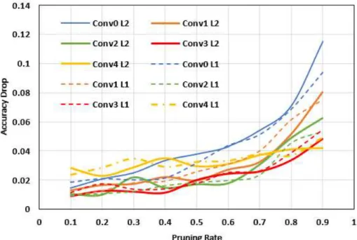
Figure 5.6. Comparison of the accuracy drop when using ℓ1 and ℓ2 regularization norms as a pruning criterion. Solid lines show the results for ℓ2 norm and dashed lines for ℓ1. ... 55
Figure 6.1. Layer characterization for convolutional layers in AlexNet trained with CIFAR-10. ... 57
Figure 6.2. AlexNet parameters in the orginal pretrained model. ... 62
Figure 6.3. AlexNet parameters in the pruned model. ... 62
Figure 6.4. AlexNet parameters in the pruned and quantized model... 65
Figure 6.5. Layer characterization for convolutional layers in AlexNet trained with CIFAR-100. ... 69
Figure 6.6. Layer characterization from conv0 to conv4 for convolutional layers in VGG16 trained with CIFAR-10... 75
Figure 6.7. Layer characterization from conv5 to conv9 for convolutional layers in VGG16 trained with CIFAR-10... 76
Figure 6.8. Layer characterization from conv5 to conv9 for convolutional layers in VGG16 trained with CIFAR-10... 76
Figure 6.9. Training accuracy during pruning with VGG16 using CIFAR-10. ... 79
Figure 6.10. Layer characterization from conv0 to conv4 for convolutional layers in VGG16 trained with CIFAR-10... 80
xiv
Figure 6.11. Layer characterization from conv5 to conv9 for convolutional layers in VGG16 trained with CIFAR-10... 81 Figure 6.12. Layer characterization from conv10 to conv12 for convolutional layers in VGG16 trained with CIFAR-10... 81
1
1. CHAPTER I
INTRODUCTION
1.1 Project motivation
Over the past few decades, machine learning has become a major field of study used in various disciplines, including finances, medicine, data mining, speech analysis and image analysis. Deep learning is based on the use of artificial neural networks that have multiple layers to extract high level features from large datasets.Convolutional Neural Networks (CNNs) nowadays are included in the wide spectrum of Deep Neural Networks (DNNs). The main advantage of CNNs compared to its predecessors is that they automatically detect the important features without any human supervision. In fact, CNNs have already surpassed human accuracy on many occasions and in different areas like image and object recognition [1] or art and style imitation [2], among others.
These architectures contain millions of parameters and, consequently, require large memory footprints and computational workloads to handle intermediate data and conduct inference. As a result, DNNs are hard to be applied to embedded devices which have limited hardware resources. For instance, the VGG-16 model, one of the most popularly used architectures in deep learning over the past few years, uses 138.34 million parameters, taking up more than 500 MB of storage space. These numbers can easily exceed the computing limit in small devices like mobile phones or even some PCs. Furthermore, as the models grow deeper, introducing more layers to achieve a better performance, the computational cost becomes even less affordable. Apart from the computational cost, assuming a device can carry out all the necessary operations
2
and has enough storage, it is very time-consuming to train a model with these characteristics to achieve a reasonable performance.
Given this situation, many researchers have focused their investigations on different techniques to compress and accelerate deep neural networks. Network model compression techniques like pruning and quantization have been proposed as efficient approaches to reduce the model redundancy without significant degradation of the performance. Parameter pruning consist in exploring the redundancy of the models and try to eliminate those parameters that can be considered uncritical or not sensitive to the performance [3]. Quantization consists in reducing the number of bits to represent parameters in a neural network [3]. The computational complexity of the network depends on the effectiveness of the pruning algorithm used in identifying and preserving the essential information from the original network.
In this thesis, a simple-yet-efficient scheme is proposed. An accuracy-aware structured filter pruning, which is based on the characterization of each convolutional layer, is combined with the quantization of fully connected layers. Among several pruning schemes, filter pruning is a naturally structured way of pruning without introducing sparsity and therefore does not require to use sparse libraries or any specialized hardware [4].
1.2 Purpose of the Study
The main goal of this work is to reduce the network size without damaging the accuracy of the original model. To accomplish the goal of this thesis, re-ordering mechanism was proposed to alter the pruning order of the layers and select the appropriate pruning rate
3
for every layer in the model. Network size and accuracy are investigated before pruning and after pruning with the proposed scheme and compared with other state-of-the-art methods in the pruning and deep compression research field.
1.3 Accuracy-aware Structured Filter Pruning Scheme
The first step of the proposed approach, named Accuracy-Aware Structured Filter Pruning, consists in performing a layer characterization, which means pruning each convolutional layer of the model individually with different pruning rates. After doing it, the accuracy results obtained when eliminating parameters from each layer using a fixed pruning rate are analyzed. According to the accuracy results, with the aim of maximizing the performance and the compression rate, an individual pruning rate is selected for each layer and layers are reordered in the final pruning for the whole model. After that quantization is applied to fully connected layers to obtain further model compression.
The analysis of the results achieved using the proposed method shows that the pruning order of the layers does affect the final accuracy of the deep neural network. Based on our experiments using the proposed pruning scheme, the parameter size of AlexNet can be reduced up to 47.28 times compared to the original model with an accuracy loss of less than 1%. Similar results are also obtained with VGG16, achieving a maximum compression rate of 35.21x.
1.4 Thesis Outline
The rest of thesis is organized in 6 more chapters. In Chapter II, an introduction to deep learning and different compression methods is provided. In Chapter III, related work is described. The general pruning method is explained in Chapter IV and the proposed
4
accuracy-aware method is detailed in Chapter V. In Chapter VI the results obtained are analyzed. Finally, in Chapter VII, conclusions and future work are included.
5
2. CHAPTER II
INTRODUCTION TO NEURAL NETWORKS AND COMPRESSION METHODS
2.1 Introduction to Deep Learning and Neural Networks Concepts 2.1.1 History
For the research on deep neural networks, it is necessary to understand the history about machine learning and deep learning. These two concepts are built around what is called Artificial Intelligence or AI which refers to the simulation of human intelligence in machines that are programmed to think like humans and mimic their actions [5]. The first artificial intelligence program was presented at the Dartmouth Summer Research Project on Artificial Intelligence (DSRPAI) hosted by John McCarthy and Marvin Minsky in 1956 and it was where Artificial Intelligence was used as a term for the first time [6]. Between 1950 and 1960, Frank Rosenblatt introduced the first model of artificial neuron, the perceptron, which eventually led to the development of the sigmoid neurons which are mostly used nowadays [7].
The machine learning concept first appeared in 1952 and was based on providing data to the machines, so they could learn how to do some task like classification without being expressly programmed for it [8]. Although AI and machine learning are both terms that appeared in the 1950s, machine learning is considered a subset of AI since it incorporates statistical methods to improve the performance. Various algorithms like decision trees, K nearest neighbors or other methods helped to make sense of machine learning until the moment when neural networks with multiple layers of neurons and the backpropagation concept appeared in 1986 [9]. However, the term “deep learning”
6
was not coined until 2006 when Geoffrey Hinton among other researchers could prove that more than a few layers could be trained using backpropagation for improved recognition in image and text [10].
2.1.2 Differences between Machine Learning and Deep Learning Machine learning can be defined as [11]:
“Algorithms that parse data, learn from that data, and then apply what they’ve learned to make informed decisions.”
Deep learning is a subset of machine learning. The main difference is that a deep learning model can determine on its own if a prediction is accurate or not using its own neural network, whereas adjustments have to be made in plain machine learning models if a prediction is inaccurate [11]. Deep Learning uses what is called Artificial Neural Networks (ANN) which architectures are inspired by the biological human brain and that capabilities go beyond what could be achieved with traditional machine learning algorithms. Therefore, deep learning does not need human intervention and the different levels of layers in the neural network apply a hierarchy in data features that allows them to learn on its own [12]. The concept of neural networks and how they work are expanded in subsection 2.1.3.
2.1.3 Artificial Neural Networks
Explaining Artificial Neural Networks would be starting with defining its fundamental unit: neurons. The word ‘neuron’ was used in this area because of the similarities with how biological neurons work. In deep learning, they are basically mathematical functions which take different inputs and these inputs are multiplied by a weight (w)
7
and have an added overall bias (b) [7]. In Figure 2.1, the basic scheme of one neuron is presented. The value of these inputs is added and passed to a non-linear or activation function, which nowadays is generally ReLU (Rectified Linear Unit), generating the output of the network. In a neural network layers of interconnected neurons will lead to a last output layer from where the final result will be obtained. The typical visual representation of a neural network is shown in Figure 2.2.
Figure 2.1. Visual representation of the neuron concept [7].
Figure 2.2. Representation of an artificial neural network [7].
Over the last years, several different models of neural networks architectures have surged like restricted Boltzmann machines (RBMs), deep belief networks (DBNs) or autoencoders (AE) [13]. All these models are used for unsupervised machine learning
8
models which means that the data used as an input for these networks is not labeled. In the thesis, the focus is on improving and optimizing deep neural networks using supervised learning, which means that datasets contain the data as well as the corresponding correct labels. During the last few years, the most common neural network architectures used for supervised learning have been Convolutional Neural Networks (CNNs) [14]. CNNs have been used for tasks regarding image classification, object detection, image segmentation and registration among others [14].
2.2 Convolutional Neural Networks
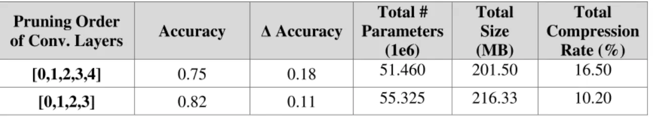
Convolutional Neural Networks or CNNs are the most popular artificial networks for image recognition and visual learning tasks. The main reason is that they can preserve local image relations while performing a reduction in its dimensions [15]. Because of this characteristic in CNNs, important features of the image can be interpreted and it allows to reduce computational complexity. The basic structure of CNNs consist of 4 types of layers: convolution layers, ReLU layers, pooling layers and fully connected layers as shown in Figure 2.3.
9
Although other types of layers can be added, these are the main steps for any CNN architecture. In the following subsections, the structure and functionality of these 4 types of layers will be explained.
2.2.1 Convolution Layers
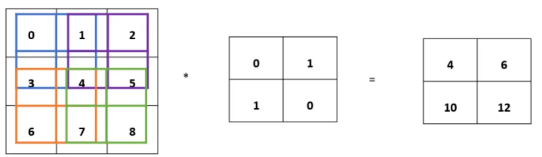
Convolution layers are always the first type of layer encountered in a CNN. They are responsible for detecting low level features of the image such as edges or curves. The input images are fed into the first convolutional layer to detect these types of features before moving to the detection of more complex shapes. Regarding how they work, convolution is understood as an operation of two functions: the pixels of the input images in their corresponding location and what is called filter or kernel [15]. At each location of the input tensor, an element-wise product is computed between the kernel and the input, adding those values to obtain the output value in the corresponding position of the output tensor [17]. After the kernel has passed through all the image, the output tensor resulting from the convolution is what is known as feature map. In Figure 2.4 and Figure 2.5, the process of convolution is shown in two and three dimensions respectively.
Figure 2.4. Convolution operation where every position of the kernel is shown in different colors.
10
Figure 2.5. Two-dimensional convolution operation with multiple input channels (Din) and multiple output channels (Dout) [16].
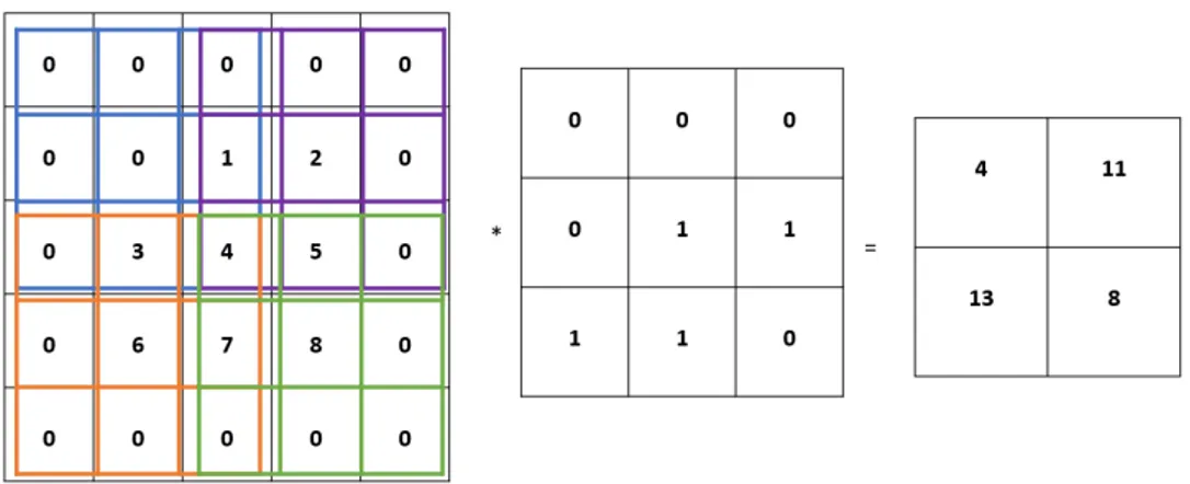
As it can be seen in Figure 2.4, the output feature map from the convolution operation has been reduced in height and width compared to the input tensor. To avoid the dimension reduction, a technique called padding is used in which rows and columns of zeros are added on each side of the input tensor [17]. By padding zeros at the image boundary, the dimensions of the image can be preserved and more layers can be added to the deep learning architecture to improve the performance. Another parameter that can be changed in convolutional layers is the stride. The stride represents the number of units by which the filter shifts through the input image [18]. Stride is normally set to 1 and it is only increased if smaller spatial dimensions and feature map down sampling is needed [17]. In Figure 2.6 and 2.7 are exemplified padding and stride respectively.
11
Figure 2.7. Convolution operation using stride=2.
The concept of convolution involves three key ideas for developing efficient machine learning architectures: sparse connections, parameter or weight sharing and invariant (or equivariant) representation [19].
-Sparse connections: In other forms of artificial neural networks, every neuron in one layer is connected to every neuron in the next layer. However, in convolutional neural networks, not every neuron in a convolutional layer is connected to the next layer and this is what is known as sparse connections [15]. This way, meaningful features (e.g., edges) of the input image do not occupy a large quantity of pixels [19]. Due to the use of sparse connectivity, the storage of a smaller number of parameters is enough to obtain a good performance with the reduced memory requirements for the model.
-Parameter (weight) sharing: In traditional neural nets prior to convolutional models, the weight values are used only once to compute the output. In convolutional neural networks, the kernel goes through all the weight input values [19]. Therefore, weights are interconnected and those changes in weight values affect to other weights in different positions. This helps to further reduce memory constraints because the number of multiplications is greatly reduced. Since the size of the kernel is smaller than the size of the input matrix and a dense matrix multiplication is not needed [19].
12
-Invariant representation: Weight or parameter sharing leads to an invariance in the input and the output function. Local feature patterns extracted by kernel movement through the input will be the same independently of which input weights are analyzed first or the order in which the output values are obtained [17].
These three ideas maximize the neural net’s efficiency and helps to make memory requirements more affordable than fully connected networks [17]. This new approach of neural nets using convolution changed the current paradigm and opened new possibilities in the world of machine learning.
2.2.2 Rectified Linear Unit (ReLU) Layers
After going through the convolution layer, an activation function is needed to extract the output. The activation function is responsible for making a non-linear transformation, so that the neural network can estimate complex functions and perform more complicated tasks [20]. Activation functions take the weighted inputs of a neuron and the added bias and apply non-linearity to finally generate the output of the neuron [21].
Nowadays the most commonly used activation function is Rectified Linear Unit or ReLU which provides the output as a linear function of the input if the input is positive while the output is 0 if the input is negative, as shown in Figure 2.8. The only activated neurons will be the ones which output is higher than 0, which means that not all the neurons will be activated at the same time by applying ReLU as an activation function [22]. When it is said that a neuron is activated, it means that the output value is propagated forward to the next layer of the network.
13
Figure 2.8. ReLU function [23].
When this first forward propagation goes through all the layers for the first time (what it is called epoch or iteration), the neural network does not give accurate predictions because the values of the weights have not been updated and in consequence the computed loss which measures how far is the result from the original classification is high. To solve this issue, an algorithm called back propagation is proposed and used in neural nets. This algorithm is based on feeding the loss obtained backwards into the previous layers, so that a more appropriate value for weights can be found. In each iteration, an optimization function called Gradient Descent will help to find the weights that will provide a smaller loss in the next epoch [24].
2.2.3 Pooling Layers
The main objective of the pooling layers between convolutional layers is reducing the size of the image (height and width) and reducing the number of parameters at the same time to achieve more efficient computations [25]. Therefore, pooling also helps to prevent over-fitting by reducing the feature maps. One of the most common forms of pooling is max-pooling. This technique takes the largest input value of the ones going through the filter or kernel. Pooling reduces the number of learnable parameters for subsequent layers, but has no learnable parameters itself, only filter size, stride and
14
padding [17]. The stride can be used for pooling to reduce the output size more. In Figure 2.9, max-pooling is exemplified.
Figure 2.9. Max-pooling operation.
2.2.4 Fully Connected or Linear Layers
Finally, the last part of CNNs are the fully connected or linear layers. The reason why it is named as fully connected or dense layers is that every neuron in the previous layer is connected to every neuron in the next layer. They are also considered a linear operation because they are one-dimensional arrays of numbers due to the flattening of the last convolutional layer. The input of fully connected layers is the output from the preceding layer and computes a probability score to classify the element into one specific class. The last fully connected layer in a neural network has the same output nodes as classification classes in the dataset used for its training. Each of these linear layers is followed by an activation function like ReLU [17].
2.3 Compression Methods
During the last few years, more accurate CNN models have been proposed but also they have grown deeper, adding more layers and making them more memory consuming
15
which requires more cost for improving their performance. However, this has caused the main problems that will be addressed in this thesis: lack of computational efficiency and difficulties meeting the memory requirements in embedded or memory-constrained devices. In consequence and specially during these last 5 years, several techniques have surged to reduce computational workloads and memory footprints by compressing neural networks maintaining the model’s accuracy. According to [3] various approaches for model compression and acceleration can be classified into five groups: low-rank factorization, Huffman coding, parameter pruning, quantization and smaller architectures. Although a brief overview of the first three categories will be given this work mainly focuses on the last group which covers structured pruning and quantization, the two techniques used for the experimental approach that will be considered.
2.3.1 Low-rank Factorization
The greatest part of the volume of computations in a CNN are convolutional layers which implies that there will be an improvement as well as an speedup regarding to the total size of the network if the number of parameters in a convolution layer are reduced [3]. The idea of reduction for convolutional layers is to identify a weight layer which is mathematically expressed as a matrix that has low rank. The weight matrixes can be represented using smaller matrixes and this will reduce the number of parameters in neural network [26]. This method can be applied to convolutional layers as well as to fully connected layers which will be a way to reduce redundancy in the weight tensors [3]. Figure 2.10 shows how one convolutional layer can be divided in two with reduced dimensions.
16
Figure 2.10. In the left the original network is shown, in the right low-rank is applied diving the previous layer in two different matrixes [3].
In [26] they only use low-rank factorization with the last fully connected layer of the network. They substitute the weight matrix of the fully connected layer (m x n) for the multiplication of two other matrices with m x r and r x n dimensions where r is the rank. As long as the number of parameters in the two matrices resulting from factorization is less than the number of parameters in the original matrix which will be a reduction in the model size. In [27] they apply low-rank factorization to divide weight matrices of all the layers in the network using singular value decomposition (SVD). They make their method scalable to an arbitrary size only by changing the selection of the rank that they use for each layer. One of the major drawbacks this technique has is that factorization is a computationally expensive operation and needs the model to be thoroughly retrained which increases the difficulty in its implementation [3].
2.3.2 Huffman Coding
Huffman coding is an algorithm used for data lossless compression of models [28]. Figure 2.11 shows an example of Huffman coding tree. This algorithm replaces the different characters that can be found among data with their corresponding code values which are bit sequences. These codes or bit sequences can have different lengths and more commonly used characters or symbols are represented with a lower number of bits
17
[29]. Codes are also generated in a way that no code is the prefix of another one. In [29] they use Huffman coding as a complement to pruning and quantization to achieve a higher network compression.
Figure 2.11. Example of Huffman coding tree [28].
2.3.3 Parameter Pruning
This method is based on detecting the redundancy of DNNs and removing the model parameters that can be considered redundant or uncritical [3]. The main idea is stablishing a criterion for pruning according to which weights will be zeroed and removed, so they are not considered in the back-propagation process [30]. The pruning process will increase the sparsity in the model. Sparsity can be defined as the number of weights in a tensor that are zero. Pruning can be performed either in convolutional or fully connected layers or in models trained from the scratch or previously trained [3]. There is a first binary classification when it comes to pruning which divides the different techniques used in this category: unstructured and structured pruning. Unstructured pruning does not follow any specific pattern or constraint for removing parameters. Although unstructured pruning can obtain better results than structured pruning, non-defined localization of the remaining parameters can cause problems in the hardware implementation [31]. Non-structured sparse networks cannot use conventional libraries
18
and need to use specialized hardware for efficient testing. Also, the random connectivity between parameters affects cache and memory access which will limit the improvement in practical acceleration [32]. On the other hand, structured pruning allows an organized sparsity which is convenient for an efficient inference and does not need any specialized deep learning libraries. Furthermore, since connections are removed in an organized way without damaging the structure of the network, other methods like quantization can be used to further compress the models [32].
The pruning can be categorized into three general types in terms of methodology: weight pruning, filter pruning and channel pruning. Weight pruning is an unstructured method in which weights are eliminated across the whole network. One of the most common criteria for eliminating weights is using the absolute values of the weights in a tensor. As shown in Figure 2.12, the absolute values are compared to a certain threshold to eliminate the ones that are below the threshold [30]. Filter and channel pruning are structured pruning methods that remove unimportant filters or channels of the model. In weight pruning, unmeaningful weight values are eliminated in all the filters because all the layers are being evaluated and compared at the same time. Opposite to weight pruning, filter and channel pruning eliminate whole filters or channels of all the layers respectively. In this type of pruning layers, either convolutional or fully connected layers or both, are being evaluated one by one or in groups depending of the framework. Then, “less important” filters or channels can be zeroed. Currently, pruning techniques use the norms like ℓ1 or ℓ2 to detect the filters with smaller norms to be pruned [33]. In fully connected layers which have no filters or kernels, it can be performed what is called neuron pruning where entire columns of weights, which represent neurons, are removed. This method can also be applied to convolutional layers and it is considered also a structured way to introduce sparsity [34].
19
Figure 2.12. Example of weight pruning where connections have been trimmed.
What differentiates channel pruning from filter pruning is the data dependency between layers [30]. In the case of filter pruning when a n number of filters are eliminated in a determined layer, the n output feature maps that had resulted from the convolution of those filters are removed too. Also, the next convolutional or linear layer will be affected because there will be n fewer input channels compared to before [30]. In channel pruning, the mechanism is very similar but n output channels from a layer would be removed first and consequently the n kernels used for the convolution that resulted in these channels will be removed too. This way, the removal of channels in one layer determines the filters being removed in the previous convolution. This dependency between filters and channels is shown in Figure 2.13.
20
Figure 2.13. From left to right the process of removal is filter pruning whereas from right to left is channel pruning.
2.3.4 Quantization
Quantization consists in reducing the number of bits to represent a number [3]. In deep learning, most common representation of weights is using a 32-bit floating point (FP32) numbers and the typical form of quantization is 8-bit integers (INT8). Low precision formats like INT8 offer advantages in terms of memory saving and speeding up operations like matrix multiplications and convolutions. Figure 2.14 shows an example of quantization mapping of real value to 8-bit integer. Also, there are much deeper quantizations as in [35] that represent weights as 4-bit or even 2-bit integers. Other networks like BinaryConnect [36] or BinaryNet [37] directly train models with 1-bit integer weights and are a type of deep neural networks in themselves called Binarized Neural Networks or BNNs. Another one of the most appealing advantages of this method is that accuracy can be maintained or if not, the accuracy drop is in most cases less than 1% with respect to the original one [38]. There are two main types of quantization: linear or uniform and non-linear or non-uniform [39]. Uniform quantization uses integers or fixed-point numbers, so computation can be performed in
21
the quantized domain (using integers). But non-uniform quantization requires dequantization for carrying out the necessary computations [39].
The most common practice, uniform quantization, can be divided into two parts: selecting a range of real numbers to be quantized and then map them into integers with the desired bit-width [39]. The selected range [α, β] of real numbers has to be mapped to a number inside the interval [–2b-1, 2b-1 – 1] where b is the selected bit-width for the integer quantization. In affine quantization, the uniform transformation function is f(x)= s · x + z, where x is the real number and s and z can be defined as:
𝑠 =2𝛼 − 𝛽𝑏− 1 (1)
𝑧 = −𝑟𝑜𝑢𝑛𝑑(𝛽 · 𝑠) − 2𝑏−1 (2)
Where s is the scale factor and z is the “zero-point” which is rounded to the closest integer value which allows to represent the real value of 0 [40]. The quantization operation can be summarized as in Equations 3 and 4 [39]:
𝑐𝑙𝑖𝑝(𝑥, 𝑙, 𝑢) {𝑥, 𝑙 ≤ 𝑥 ≤ 𝑢𝑙, 𝑥 < 𝑙
𝑢, 𝑥 > 𝑢 (3)
𝑥𝑞= 𝑞𝑢𝑎𝑛𝑡𝑖𝑧𝑒(𝑥, 𝑏, 𝑠, 𝑧) =
= 𝑐𝑙𝑖𝑝(𝑟𝑜𝑢𝑛𝑑(𝑠 · 𝑥 + 𝑧), −2𝑏−1, −2𝑏−1− 1) (4) Usually, quantization is a technique that is applied after the neural network’s training although other modalities like quantization aware training can be implemented [41].
22
Figure 2.14. Quantization mapping of real value to 8-bit integers [39].
2.3.5 Design of smaller architectures
The four methods explained in prior subsections compress deep neural networks and reduce the number of parameters, but their architecture, the number and orders of the layers are remaining the same. A way to reduce the weights in a CNN is using filter decomposition which consists of replacing big convolutional layers by more convolution layers and smaller filters [38].
Apart from these methods, it also exists the possibility of making a new architecture from the scratch which is the case of SqueezeNet [42] or MobileNet [43]. SqueezeNet was created having in mind obtaining a comparable or even better performance than state-of-the-art deep neural networks like AlexNet or VGG using a smaller quantity of parameters. SqueezeNet achieved the expected compression since it is 50x smaller than AlexNet having the same performance in ImageNet dataset. With MobileNet, researchers wanted to reduce the number of operations used in SqueezeNet and they also obtained a better accuracy in ImageNet [38].
2.4 Transfer Learning
Another deep learning concept that is related to the work presented in this thesis is transfer learning. Transfer learning consists in using networks previously trained in
23
large datasets (e.g., ImageNet) and then retraining the model with a smaller dataset or directly use it for inference if both datasets are similar enough [25]. One reason for using transfer learning is that it is difficult to obtain a well-classified large dataset in some fields like bioinformatics, so transfer learning allows testing data to be different from training data [44]. Furthermore, even if the necessary amount of data to train a deep learning model from scratch is available training a deep model can take a long time depending on the number of layers used in the network and the size of the dataset. Also, transfer learning is used to improve the performance by transferring the knowledge obtained through its first training, so that when the network is retrained with the new dataset less iterations are needed. Since initial weights are not random with transfer learning and they have already been trained, the performance of the network is likely to improve.
The two basic types of transfer learning are fine tuning and feature extraction. In fine tuning, the whole network or at least one or more convolutional layers are retrained by updating the weight value through backpropagation. On the other hand, in feature extraction, only the last fully connected layers will be adapted to the number of categories in the new dataset and retrained while all the other weights in the rest of the layers can be considered to be frozen [25].
24
3. CHAPTER III
RELATED WORK
3.1 Network Pruning
In 2015, Han [45] introduced a simple pruning strategy: all connections with weights below a threshold should be removed. This process had to be followed by fine-tuning to recover the accuracy lost by eliminating weights. This was the research work which introduced weight pruning as a technique for CNN compression. However, this first attempt created a non-structured and very sparse model which could not be supported by mostly used libraries and ignored main memory and cache memory limitations. To avoid limitations of non-structured pruning, other researchers as in [32] argued that filter level pruning is a better option. In [32] they propose a compressed model called ThiNet to prune the unimportant filters to simultaneously accelerate and compress CNN models in both training and test stages with minor performance degradation. Also, the versatility of pruning is shown as it is perfectly compatible with other post processing methods like gcos (Group Convolution with Shuffling), the one they used, to achieve a higher compression of the model.
Published in 2017, [33] is one of the mostly cited references in the pruning filter research field [4], [32], [46], [47], [48]. In [32], they use the same fixed pruning rate for all the layers and do not stablish a criterion for obtaining a good pruning ratio for each of them individually. On the contrary, Li [33] studied the effect of pruning sensitivity to decide the different pruning rate for each convolutional layers. For layers that were particularly sensitive to pruning, significantly lowering the accuracy of the network when pruned, they reduced the pruning rate or even skipped them in the pruning
25
schedule. Li’s methods achieved a 34% compression in VGG16 and a 64% parameter reduction maintaining an accuracy close to the original baseline.
[33] also includes two concepts which are independent pruning and greedy or layer wise pruning. Independent pruning does not account for the filters removed in the current layer when retraining the next layer while greedy does. The greedy layer-wise approach has been used in [32] throughout the pruning stage. But in [49] channels are eliminated greedily after analyzing each layer and evaluating their weights using LASSO regression.
Another filter pruning model is introduced in [47] which uses what they call an adaptive filter pruning module where they prune filters according to the value given by a pruning rate controller. It constantly evaluates accuracy, so that the accuracy does not go below a certain threshold. This principle is very similar to the algorithm that will be used in this thesis to maintain accuracy in convolutional layers when deciding the pruning rate for each of them.
Other works have novel contributions in terms of filter selection criteria. In [4], they use their own algorithm, called AULM (Alternative Updating with Lagrange Multipliers), to decide which filters are considered unimportant. Through multiple iterations, they try to optimize the result of the combination of two different regularizers (ℓ2,1 and ℓ2,0) to achieve structured sparsity. In [50] they propose a modified ℓ1,2 norm penalty to increase the sparsity of pretrained models maintaining a good model performance. In [51]they use the k means algorithm to find out which filters are more convenient to prune in the deep neural network. This way, they get the relationships of similarity among filters and only leave without pruning those closer to the centroid of the cluster. Also, in [52] they propose a criteria based on the covariance and correlation of filters in convolutional and fully connected layers and successfully compressed
26
different state-of-the-art models. Even though nowadays most typical criteria chosen by researchers are still the absolute value of weights, l1 and l2norms [53].
As it can be inferred from previous examples, researchers have developed different strategies to address the problem of network compression using pruning, but there is still room for improvement in terms of compression and acceleration results.
3.2 Pruning and Quantization Combination
To achieve further compression, some research works have implemented post training quantization after pruning. In [29] they achieve a 35x AlexNet compression and a 49x VGG16 reduction in size using a compression pipeline with three stages: weight pruning, quantization and Huffman coding. Another method that benefits from the combination of pruning and quantization is CLIP-Q [54] which incorporates weight unstructured pruning and quantization. They allow flexible pruning adapting decisions over time as their network structure changes when starting to prune layers and have a parallel pipeline to perform pruning, quantization and fine tuning at the same time. In [55] a combination of quantization and weight pruning is introduced. They are trying this method in newer convolutional neural networks like ShuffleNet [56] and MobileNet [43]. In our line of work at the beginning of 2020, Guerra [57] proposed a pruning strategy for already quantized neural networks using Bayesian optimization to determine the pruning ratio for each layer. For evaluating filter similarities, they used Euclidean and cosine distance, being these metrics their criteria for filter removal. One noticeable problem with most of the models previously mentioned is the number of epochs required for retraining the model after pruning. In [57] they use 60 epochs for retraining which in large models like VGG-16 can take several days for finishing the process, but others like [58] use up to 400 iterations. In the thesis, our approach will
27
include one parameter that has not been mentioned in the literature yet: the retraining order of the layers. How this parameter can affect the fine-tuning process and the accuracy when a smaller number of epochs is being used will be described in this thesis.
28
4. CHAPTER IV
GENERAL PRUNING SCHEME
In this chapter, a general overview for the typical pruning scheme along with some of its variants will be presented. According to [53], the pruning scheme can be divided in 3 main stages: model training and objective selection, pruning itself and fine-tuning. Following this organization, which is used in many research works, all the necessary elements for generating a pruning scheme will be exposed.
4.1 Model training and Objective Selection
The first step to start a pruning pipeline is to train a model. As it was explained in Section 2.3.3 of Chapter II, pruning consists in removing parameters that can be considered redundant or unimportant. To identify which parameters meet these requirements, training of the model is required. When a model is being trained for the first time, weights are set randomly and, consequently, it is not possible to analyze their value and evaluate them if the model has not been trained before. When the model has been trained, weight values in every layer are defined and can effectively be analyzed according to the selected criteria. Here is where the use of transfer learning, mentioned in Section 2.4 of Chapter II, makes sense in this framework. A pretrained network using a large dataset like ImageNet [59] which requires an extensive training process helps saving time in the pruning framework because there is no need to retrain the network from scratch. However, some works still prefer to train networks from scratch to avoid the dependence in pretrained models [60].
29
Once the model is trained, it is needed to define a pruning target. Pruning targets are directly related to the final aim of the final pruned model. Network compression can help improving different types of parameters depending on where it is applied. Although the main reason for pruning is also compressing networks for their implementation in embedded devices, we can expect three types of major improvements: reduction in model size, faster inference time and reduction in the number of computational operations [61]. Depending on the final goal, the process of pruning can focus more on one or more of these advantages. When pruning only affects convolutional layers, computational power is reduced. This type of layers is the most computationally expensive as they require of the use of several matrix multiplications in the convolution process and other calculations related to the stride and padding. This does not mean that there will not be a parameter reduction when only convolutional layers are being pruned, but in CNNs majority of the parameters are found in fully connected layers. Therefore, when linear layers are pruned, the model’s compression rate can potentially be much higher. Then, to achieve highly reduced number of parameters while also reducing the computational complexity, pruning it fully, both convolutional and linear layers in the same framework, is the best option. Once the model has been trained and the targeted layers are selected, the next step is to apply pruning itself.
4.2 Pruning
The main task in pruning consists in taking out redundant or unimportant parameters, but there are three different aspects that need to be addressed to determine how is exactly pruning going to be applied.
30 4.2.1 Pruning Level
Pruning level refers to what type of parameters are going to be pruned. As it has been mentioned in Section 2.3.3, there are three main types of pruning: weight pruning, filter pruning and channel pruning. These methods can be used individually or as a combination like in [62] where both weight pruning and filter pruning are combined to achieve better compression results. As weight pruning is an unstructured way of pruning that requires the use of specialized libraries and the support of embedded devices, very limited filter and channel pruning are often proposed to solve this problem [46]. Pruning level can also be variable and changed during the pruning process, depending on how the proposed approach intends to work over the network and what type of results are being prioritized. What will determine the acceleration and compression success maintaining the performance of the network is how is the importance of these parameters weighted with the corresponding pruning criterion
4.2.2 Pruning Criteria
The importance of the type parameters chosen to prune has to be evaluated, so that the “unimportant” ones can be detected and removed. It is also important to define what can be understood as “unimportant” or “redundant”. As a solution, in the research literature, multiple types of criteria have been proposed. One of the most popular and the simplest criteria is the absolute sum of weights which can be used to decide the removal priority of parameters. Weights that have a lower absolute value are supposed to have a lighter impact on the final classification of the network, so they are susceptible of being removed first.
31
Another common strategy is to use ℓ1 or ℓ2 norms as a criterion for selection. A norm can be defined mathematically as the distance function between two vectors 𝑥 and 𝑦 . The most common vector norms, ‖𝑥‖𝑝 or p-norms, given a vector 𝑥 with 𝑖 elements can be expressed as in equation (5) [63]:
‖𝑥‖𝑝 = (∑|𝑥𝑖| 𝑖 𝑝 ) 1 𝑝 (5)
The most popularly used norms as it has been mentioned are ℓ1and ℓ2 norms. Both are explained graphically in Figure 4.1. ℓ1 is also known as Manhattan or taxicab distance and measures the smallest distance between two points as the sum of the absolute difference of their Cartesian coordinates. If 𝑝 = 1 equation (5) can be rewritten as:
‖𝑥‖1 = ∑|𝑥𝑖| 𝑖
= |𝑥0| + |𝑥1| + ⋯ + |𝑥𝑖| (6)
ℓ2 is known as Euclidean distance and measures the smallest distance between two points as the sum of the squared difference of their coordinates. If 𝑝 = 2 equation (5) can be rewritten as:
‖𝑥‖2 = √(∑ 𝑥𝑖2 𝑖
) = √𝑥02+ 𝑥
32
Figure 4.1 In red, yellow and blue ℓ1 norm or Manhattan distance is represented while in green ℓ2 norm or Euclidean distance is displayed [67].
Although these norms are also used in practice for regularization purposes to avoid overfitting, they are also widely used in pruning as a method to select the most irrelevant parameters. In [33], after several experiments, they could see how pruning filters with the smallest ℓ1 norm led to better results compared to removing random filters or the largest ones.
There are other methods that are not commonly used, but those schemes are equally valid to select which concrete parameters need to be pruned. For example, in [64], they introduce the Average Percentage of Zeros (APoZ) to evaluate the importance of a neuron measuring the percentage of zero activations of a neuron after the ReLU mapping. Other examples of different criteria can be found in and are explained in detail in Section 3.1 of Chapter III.Many pruning frameworks are available in deep learning research, so it is a common practice to propose different pruning criteria as a novelty.
4.2.3 Pruning Algorithm
When pruning level and criteria are defined, the last step of pruning is selecting which algorithm or how exactly are these selected parameters going to be removed. As
33
explained in [53], three aspects of the pruning algorithm can be detailed: the removing strategy, the searching algorithm and pruning rate. In the removing strategy, it can be specified the order of removal of the elements like if, for example, more than one type of pruning with different criteria is being used or, if parameters are being removed by layers, choosing which layer is removed first. Also, it is detailed if some additional steps like fine-tuning or even other compressing methods are required before or after removing any elements. The searching algorithm refers to the type of strategy used to come to an optimal solution. The two main types of searching algorithms that we can find in the literature are greedy or reinforcement learning. In greedy approaches, the most unimportant parameters are searched layer-wise or group-wise to achieve a certain level of sparsity. On the other hand, a reward function is used in reinforcement learning, so that the network itself can come to the optimal solution based on the functions’ parameters which are sparsity level and text accuracy [65]. Finally, pruning rate is the percentage of weights, filters or channels that is being taken out to achieve a certain level of total or local sparsity depending on the framework. An adequate pruning rate will allow an accuracy recover despite removing parameters of the model [53]. Pruning rate can be fixed like in [32] or variable depending on the layer [33]. Pruning rate can be even changed after a certain number of iteration with the aim of reaching a final pruning goal without damaging the network’s accuracy [66].
4.3 Fine-tuning
After pruning a network model, it is essential to retrain the network to recover the accuracy lost during the pruning stage. This process of retraining is what is known as fine-tuning which has also been described in Section 2.4 of Chapter II. It is also associated with transfer learning, although it can be performed with either pretrained or
34
not pretrained networks.Fine-tuning can be performed in each layer or group of layers after every pruning step is done or at the end when the whole model has been pruned. Also, after pruning process, there is usually an evaluation process to see if the test accuracy or other possible constraints have been met. In case that the answer is negative, fine-tuning is performed again until the set goals are achieved. The number of epochs for retraining, the learning rate or the optimizer used are decisions the programmer has to make heuristically in order to ensure an optimal outcome.
35
5. CHAPTER V
PROPOSED METHOD
In this chapter, the proposed method is addressed. Firstly, we describe the filter pruning technique used for initial compression through the characterization of individual layers. Then we explain how the pruning rate and the order of the layers are selected. Finally, we describe the use of quantization in fully connected layers to achieve a further compression while maintaining the model’s accuracy. Figure 5.1 shows overall flow of the proposed approach.
Figure 5.1. Proposed method framework.
First a sweep pruning each layer individually is done. After that, certain information extracted from the layer characterization is used as an input for the pruning schedule algorithm. With the results from the pruning algorithm the pruning process for the whole model can start. One layer is pruned at a time and after the model is fine-tuned for a determined number of epochs. When all convolutional layers are pruned, quantization is applied to the linear layers. All this process leads to the final pruned model.
36
We consider a CNN network with L convolutional layers. The weight matrix in each layer, 𝑊𝑖, can be expressed as 𝑊𝑖 ∈ ℝ𝑁𝑖+1×𝑁𝑖×𝑘×𝑘where 𝑁𝑖 denotes the number of input channels of convolutional layer 𝑖 and 𝑁𝑖+1 next layer’s number of input channels, which is the same as the number of output channels for layer 𝑖. The constant 𝑘 represents the kernel dimension considering that height and width are the same. Kernels can be represented as 𝒦 ∈ ℝ𝑘×𝑘. Every filter 𝑗 in layer 𝑖 can be expressed as ℱ𝑖,𝑗 ∈ ℝ𝑁𝑖×𝑘×𝑘. The pruning rate for each layer will be represented with 𝒫𝑖.
After the theoretical framework, the first experiments that were conducted to develop what is the final proposed method will be explained. Finally, in this chapter, the use of ℓ1 and ℓ2 norms as a filter selection criterion is addressed.
5.1 Filter Pruning
The first step of the proposed method is applying filter pruning. The process consists in identifying those filters which can be considered unimportant or redundant, so that they can be eliminated. To identify redundant filters, the importance of the filters needs to be evaluated according to a criterion. After evaluating different norms through our experiments, we select ℓ2 norm also known as Euclidean norm as a criterion:
‖ℱ𝑖,𝑗‖2= √∑ ∑ ∑|ℱ𝑖,𝑗(𝑛, 𝑘, 𝑘)|2 𝐾 𝑘=1 𝐾 𝑘=1 𝑁𝑖 𝑛=1 2 (8)
Evaluating each layer of the CNN model, we can rank the filters assuming the ones with a smaller norm will lead to lower activation values and consequently a less impact in the final classification. Filter selection for every layer using pruning with ℓ2 norm can be formulated mathematically as:
37
∀𝑖 ∈ {1, … , 𝐿}: min ℓ2(ℱ𝑖,𝑗) j ∈ 𝑆
𝑠. 𝑡 𝑆 ⊂ {1, … 𝑁𝑖+1} , 𝑁(𝑆) = 𝑁𝑖+1× 𝒫𝑖
(9)
𝑆 represents a subset of all the possible output channels and 𝑁(𝑆) is the total number of elements in subset 𝑆 which is also the number of filters that will be pruned. After pruning the selected filters in layer 𝑖, we will fine-tune the model retraining it for a determined number of epochs. Following a greedy layer-wise approach, the same process will be continued with layer 𝑖 + 1. This process will keep going until 𝑖 = 𝐿. In Figure 5.2, it is shown in detail how the process of filter pruning affects the weights in CNN convolutional layers.
Figure 5.2. Elimination of filters in one layer through pruning causes the elimination of output channels which will not be an input for next layer.
Before moving to final pruning stage, pruning sensitivity for every layer will be investigated. The accuracy values obtained during the sweeping will be used to decide which pruning order will be the best and what will be an adequate pruning rate for each layer.
38 5.2 Pruning Schedule Algorithm
In the proposed pruning schedule algorithm, a final pruning rate 𝒫𝑖 for every layer will be determined according to ℓ2 norm criteria. We will perform a sweep to characterize every layer going from 𝒫𝑚𝑖𝑛 = 0.1 to 𝒫𝑚𝑎𝑥 = 0.9 with a step size of 0.1. As a result, only 𝑁𝑖+1 × 𝒫𝑖 among the 𝑁𝑖+1 channels will be removed which means that the final number of output channels in layer 𝑖 will be 𝑁𝑖+1 × (1 − 𝒫𝑖).
To characterize individual layers, we keep changing the pruning rate from 𝒫𝑚𝑖𝑛 to 𝒫𝑚𝑎𝑥 until all corresponding accuracy values are obtained from pruning each layer. Once the sweep is completed, enough information will be ready to apply Algorithm 1 which is proposed in this paper. The aim of the algorithm is to achieve the maximum compression rate of the model while minimizing the accuracy loss. To achieve the goal, it is necessary to set a different pruning rate for every layer.
In Algorithm 1, we are comparing the accuracy result when pruning a layer of the model with a certain 𝒫𝑖 to the baseline accuracy of the original model. To avoid the algorithm from being excessively restrictive, which would lead to leaving most or all the layers unpruned, the threshold is multiplied by a factor that goes from 0.985 to 0.997 depending on the model and dataset. These values have been determined experimentally to balance the trade-off between accuracy and compression results. The original accuracy multiplied by this factor is what we consider as the threshold.
In case that the accuracy of any layer is lower than the threshold, the corresponding layer will not be pruned. If the threshold is set too low, the accuracy of the model when retraining will be significantly lower compared to the original, but the compression rate of the model will be high. However, if the threshold is set too high, the testing accuracy of the new model will also be higher, but the compression rate will drop. Several
39
experiments have been done with two different models and what could be noticed empirically in deeper models is that threshold needs to be closer to the original accuracy to obtain a high accuracy in the final model. This occurs because when the model has more layers being pruned and retrained the accuracy loss in the final model is likely to add up and be higher. That is why AlexNet compression rate is higher than in VGG16. Applying Algorithm 1, we obtain the maximum pruning rate for which every layer has an accuracy that is equal or higher than the threshold. According to individual layer’s accuracy, layers will be re-ordered in descending order.
Algorithm 1: Order and 𝒫𝑖 for Convolutional Layers
Input: List of test accuracies and corresponding pruning rate for each layer; List of convolutional layers in the model.
Output: Ordered list of convolutional layers and their 𝒫𝑖. 1. for each l in [1, L] do:
2. for each 𝒫 in [𝒫𝑚𝑖𝑛, 𝒫𝑚𝑎𝑥] do:
3. if testing accuracy ≥ threshold: 4. layer, pruning rate ← l, 𝒫
5. else:
6. layer, pruning rate ←not found 7. end
8. end
![Figure 2.3. Convolutional Neural Network (CNN) [16].](https://thumb-eu.123doks.com/thumbv2/5dokorg/4331046.98098/23.892.172.770.803.1093/figure-convolutional-neural-network-cnn.webp)