Heuristiska algoritmer för schemaläggning i real-tidssystem med hänsyn till data beroenden

(1)

Heuristic minimization of data latency in offline

scheduling of periodic real-time jobs

Department of Mathematics, Linköping University Ariyan Abdulla & Erik Andersson

LiTH-MAT-EX--2018/01--SE

Credits: 16 hp Level: G2

Supervisors: Elina Rönnberg,

Department of Mathematics, Linköping University Mikael Asplund,

Department of Computer and Information Science, Linköping University Mattias Gålnander,

Arcticus Systems AB Examiner: Elina Rönnberg,

Department of Mathematics, Linköping University Linköping: January 2018

(2)

(3)

Abdulla & Andersson, 2018.

Abstract

The schedule for the jobs in a real-time system can have a huge impact on how the system behave. Since real-time systems are common in safety applications it is important that the scheduling is done in a valid way. Furthermore, one can enhance the performance of the applications by minimizing data latency and jitter. A challenge is that jobs in real-time systems usually have complex constraints making it too time consuming to minimize data latency and jitter to optimality. The purpose of this report is to investigate the possibility of creating high quality schedules using heuristics, with the goal to keep the computational time under one minute. This will be done by comparing three different algorithms that will be used on real scheduling instances provided by the company Arcticus. The first algorithm is a greedy heuristic, the second one a local search and the third one is a metaheuristic, simulated annealing. The results indicate that the data latency can be reduced whilst keeping the computational time below one minute.

Keywords: Scheduling, heuristics, data latency, jitter, single-processor scheduling URL for electronic version:

(4)

Acknowledgements

We would like to thank Elina Rönnberg and Mikael Asplund for supervising this project. Without their assistance the work would not have been able to complete in such a successful way. We would also like to thank Mattias Gålnander and the employees at Arcticus for giving us the opportunity to work with this project and for their contribution whenever we needed help. We would also like to send thanks to Julia Knave for sharing ideas and for her support.

(5)

C

ONTENTS

1 Introduction ... 1 1.1 Background ... 2 1.2 Purpose ... 2 1.3 Goal ... 2 1.4 Method ... 2 1.5 Limitation ... 3 1.6 Structure ... 3 2 Theory ... 5 2.1 Real-time systems ... 5

2.1.1 Background to real-time systems ... 5

2.1.2 Definition of our scheduling problem ... 5

2.1.3 Attributes of a job and a schedule ... 6

2.1.4 Dependencies between jobs ... 8

2.1.5 Placing jobs in the schedule ... 9

2.1.6 Data latency and jitter ... 9

2.2 Optimization in real-time systems ... 12

2.2.1 Scheduler and schedules/schedule ... 12

2.2.2 Scheduler optimality ... 12

2.2.3 Schedule optimality ... 12

2.2.4 Algorithms for scheduling in real-time systems ... 12

2.3 Optimization/Heuristics... 14

2.3.1 What is combinatorial optimization? ... 14

2.3.2 Time complexity ... 14

2.3.3 Search space ... 14

2.3.4 Heuristics ... 15

3 Problem formulation ... 21

3.1 How the different jobs are translated to nodes... 21

3.2 Nodes grouped in buckets ... 21

3.3 The schedule ... 23

3.4 The neighbourhood ... 23

3.5 Evaluation measures... 23

4 The three algorithms that have been studied ... 25

(6)

4.1.1 Keeping schedule valid ... 25

4.1.2 Critical path ... 25

4.1.3 Bucket order ... 27

4.1.4 Iteration through buckets ... 27

4.1.5 Pseudocode for greedy constructive algorithm ... 28

4.2 Local search algorithm ... 28

4.2.1 Minimizing the data latency ... 29

4.2.2 Evaluation of spots in-between jobs ... 29

4.2.3 Rearrangement of jobs after completion of schedule ... 29

4.2.4 Pseudocode for local search algorithm ... 30

4.3 Simulated Annealing ... 31

4.3.1 Initial solution ... 31

4.3.2 Evaluation and placement of jobs ... 31

4.3.3 Benefits of making non-greedy job rearrangements ... 32

4.3.4 Pseudocode for SA algorithm ... 34

5 Result ... 35

5.1 The instances to be scheduled ... 35

5.1.1 Easy problem ... 35

5.1.2 Hard problem ... 35

5.1.3 The real problem ... 36

5.2 Results from the algorithms ... 36

5.2.1 Easy problem ... 36

5.2.2 Hard problem ... 38

5.2.3 The real problem ... 39

6 Discussion and Conclusion ... 45

6.1 Trade-off between data latency and jitter ... 45

6.2 Same algorithms with less time complexity? ... 45

6.3 Ambiguity of results ... 45

6.4 Conclusion ... 46

(7)

1 | P a g e Abdulla & Andersson, 2018.

1 Introduction

In modern vehicles, a large part of innovation and customer value is based on advanced computer-controlled functionality such as air condition and airbag. According to a recent study made by Mubeen et al., 2017, the size and complexity of the vehicle software has increased significantly since its

introduction. For example, the software in a car used to consist of hundred lines of code in the late 70s, now it can consist of more than a hundred million lines of code. The authors further point out that since modern vehicles have a high standard of safety, many functions within them needs to adhere to a safety-critical nature with real-time requirements.

The braking system of a car is an example of such a function that have real-time requirements. We can think of the braking system as having a sensor that reads inputs from the brake pedal periodically, for example every five milliseconds. In the normal case, when the pedal is not pressed down, nothing will happen in terms of producing output from the system, in other words the car does not slow down. At some point, the pedal will be pressed and the consequence of this is that the input from the sensor will be propagated through a chain of jobs in the computerised control units to produce an expected output, such as making the car to slow down. A job is a unit of work that is scheduled and executed by the system. Since the timing requirements are critical, each job in a real-time system must complete its work periodically. Because the sensor is reading the input from the brake pedal periodically the jobs in the earlier example will be executed at least once every fifth millisecond. And from a safety perspective, it is critical that these functions produce a correct output within an acceptable time span.

For example, the real-time system in the previous example would work by executing a predetermined sequence of jobs. How the jobs are placed in the queue for execution, dictates how long it will take the data to propagate from input to output. This will present itself by the time it will take from the pedal pressing to the actual breaking. The order in which the jobs are placed therefore have a direct influence on the correctness of the output and how fast it is produced.

In the design of real-time systems each job needs to be associated with timing constraints and dependency fulfilments. Some constraints are more important than others. For instance, jobs must be scheduled in an order that ensures that output is produced correctly and within the time required. This is a requirement for all real-time systems.

Another possible constraint is to keep the data latency sufficiently small, which is the time it takes for data to propagate between jobs. A system can also be designed to have reduced amount of jitter, which is the irregularity of job executions after each repeated period. This report will suggest heuristics that aims at minimizing data latency and how it affects jitter, without violating the critical constraints.

(8)

1.1 BACKGROUND

Arcticus Systems AB is a company located in Sweden that delivers and supports state-of-the-art safety critical embedded real-time system products and services. Rubus® is the name of one of their products that schedules jobs, with different timing properties. This is done pre-runtime, meaning a schedule is produced before the application is executed. One way to create the schedule is via heuristic based off-line scheduling algorithms. Depending on the kind of algorithm, the resulting schedules can be of different qualities and there can be a difference in the time it takes to produce the schedule.

Arcticus Systems AB are interested in investigating if it is possible to employ optimization techniques to create schedules that minimizes or at least reduces data latency, which is a measurement that is relevant from a performance perspective. This should be done without disrupting the timing requirements of the schedule. Also, the algorithm needs to be time efficient as it will be executed in a developer desktop where a person is waiting for the result. In practice, this means that a schedule should be produced within one minute.

1.2 PURPOSE

The purpose of this thesis is to investigate if data latency can be reduced and how this affect the total jitter when creating a schedule while at the same time keeping the computational time in a single processor under one minute. This will be done by designing a local search method and a metaheuristic and compare them to an existing constructive greedy heuristic.

1.3 GOAL

The goal is to create a heuristic based scheduler and present it in this report in the form of pseudocode, so that it can be integrated into Rubus®. The requirements are that the run times of the scheduler is under one minute and that the heuristic strives at minimizing the jobs data latency.

1.4 METHOD

Arcticus is the main stakeholder in this project and therefore the problem specification has been motivated by the current needs of Arcticus. Arcticus have an extensive knowledge within real-time systems and therefore meetings and continuous communication was arranged to further advance within the subject of matter.

The problem was then represented in a form that is suitable for this thesis. This means that the way Arcticus defines a job and all its attributes was translated in a way so that the same information could be used for programming. This is important because the heuristic scheduling algorithm was prototyped with programming tools such as Python.

Arcticus has a scheduler based on a constructive greedy heuristic that always produces a valid schedule but without minimizing data latency and jitter. This scheduler was the first to be implemented to act as a reference point for the latter heuristics.

(9)

Following the first scheduler, a second scheduler was implemented with the goal of rapidly creating a schedule and at the same time minimizing data latency using a constructive greedy heuristic and a local search heuristic. This was done by incrementally improving the first algorithm. Direct feedback of improvement could be seen since the algorithm can be applied on a scheduling problem that Arcticus has provided. This scheduler was evaluated against the first scheduler to see if progress has been made. The evaluation was based on whether data latency has been reduced and if the requirement of keeping the run time under one minute is being fulfilled. At the same time the total change in jitter was evaluated.

The third algorithm was based on the same heuristic techniques as the second algorithm but extended to a metaheuristic, more specifically simulated annealing. This algorithm was evaluated against the first and second one to see if progress had been made. The evaluation was based on whether data latency had been reduced, but without considering the requirement of keeping the run time under one minute. At the same time the total change in jitter was evaluated. This allows us to evaluate whether the algorithm works better if it is given more time to create a schedule.

1.5 LIMITATION

This report will not investigate an optimal placement of jobs with respect to minimizing data latency because it is likely that it would yield an unreasonably long computational time. As future work, it would be of interest to compare an optimal placement of jobs with heuristically produced schedules. But since Arcticus are interested in a fast scheduler, our focus will be on applying heuristics techniques.

1.6 STRUCTURE

The report is divided into six chapters, the first one being the introduction to the problem. The second chapter will give insight to the concepts within real-time systems, optimization in real-time systems and heuristics. The third chapter will present a model of the scheduling problem. Chapter four will describe the design of the three different algorithms. Finally, chapter five and six will present the results and a conclusion.

(10)

(11)

2 T

HEORY

The theoretical basis required to understand the concepts presented in this thesis will be presented in this chapter. The structure of the chapter is such that first an introduction to real-time systems and related concepts are presented. After this, optimality within real-time system will be discussed. Lastly our main subject, which is within another discipline of science, will be explored, namely the concepts of

mathematical optimization.

2.1 REAL-TIME SYSTEMS

This chapter will begin by giving some background of real-time systems. It will discuss the different concepts that are crucial in real-time systems and for understanding the scheduling problem. Towards the end there will be a more detailed description of the timing requirements that must be met by the heuristic algorithms described in this report and a description of how to calculate values for schedule evaluation.

2.1.1 Background to real-time systems

A real-time system is a system that is not only dependent on the logical result, the output, in terms of the correctness of the system, but also on the time at which the output is produced.

According to Buttazzo, (1997), the reason why real-time systems is of importance is that in the physical world there must be a physical effect within a chosen time-frame, for example the release of an airbag. A real-time system usually consists of a controlling system, often a computer, and a controlled system, the environment. The controlling and controlled system are integrated, and the controlling system interacts with its surroundings depending on what information is available about the environment.

A job in a real-time system can have several different timing properties. This report will only consider the attributes that Arcticus use to characterize their jobs. The most typical timing properties, according to Mohammadi & Akl, (2005), are release time, which refers to the time at which a job is ready for

processing, deadline, which refers to time by which execution of the job should be completed, and worst-case execution time, which refers to the maximum time it takes to complete a specific job after the job is released. The authors explain that system failure will occur if the timing constraints are not met, meaning that these timing behaviours requires that the system is predictable. Predictability means that it should be possible to determine a job's completion time with certainty when it is activated.

2.1.2 Definition of our scheduling problem

The scheduling problem is about determining a schedule, for the execution of jobs so that they are all completed before the overall deadline. The appropriate scheduling approach depends on the properties of the system and on the kind of jobs in a given real-time system. There are different properties to consider and this report will only mention the properties that occurs in Arcticus' real-time system. These are explained by Arcticus, (2017) and J. W. S. Liu, (2000) as:

 Hard real-time jobs

This means that all jobs must be executed before their deadline. In contrast, soft real-time jobs can have their deadlines surpassed without larger consequences.

 Periodic jobs

These are jobs that are activated regularly at fixed rates, in other words periods. This means that job instances must be executed once every period.

(12)

 Trigger Independent/dependent jobs

A trigger is a job that must be executed before the job it “triggers”. If a job is trigger dependent it means that all its preceding triggers must have been executed before it starts its own execution. In Arcticus' real-time system, jobs can either be trigger independent or trigger dependent.

 Data Independent/dependent jobs

If a job is data dependent it means that it gets data from another job in the system. The difference here from the trigger dependent job is that jobs can start their execution without receiving any data, this will be further explained in chapter 2.1.4. In Arcticus' real-time system jobs can either be data independent or data dependent.

 Offline scheduling

This means that the schedule will be created pre-runtime.

Given this information, the problem can be defined as: create a schedule offline with periodic hard real-time jobs that are trigger and data dependent.

2.1.3 Attributes of a job and a schedule

Below are the attributes that characterize a job or a schedule according to J. W. S. Liu, (2000) and/or Arcticus, (2017).

Jobs

The set 𝕁 contains all unique jobs to be scheduled. The notation 𝐽𝑖∈ 𝕁 is used to describe each unique job

𝐽𝑖 where 𝑖 = 1,2,3, . . . , |𝕁| This means that 𝐽1 is the first job, 𝐽2 is the second job and so on. Each job 𝐽𝑖 has

a period 𝑃𝑖. Given the set of these jobs there are several copies of each job that is repeated periodically.

These copies are called job instances. With these job instances, a repeating schedule can be created.

Job instance and period

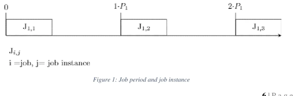
The period of a job is the time between repetitions of that job. Because each job has a period, then multiple instances of each job exist. Each job instance 𝐽𝑖,𝑗, is an entity represented by its own deadline,

worst case execution time (WCET) and some dependencies to other job instances. 𝐽𝐼 is the set of all the job instances. For example, consider 𝐽1 with period of 5 𝑚𝑠. This means that 𝐽1 must be executed every

5 𝑚𝑠. If the total repeating cycle is 15 𝑚𝑠, then 𝐽1,1 would be the first instance between 0 𝑚𝑠 och 5 𝑚𝑠,

𝐽1,2 the second instance between 5 𝑚𝑠 and 10 𝑚𝑠 and 𝐽1,3 the third instance between 10 𝑚𝑠 och 15 𝑚𝑠.

, shows how a job, in this example 𝐽1, must be repeated once every 𝑃1. In the time frame between zero

and 𝑃1, 𝐽1,1 must be executed once. Between 𝑃1 and 2 ∗ 𝑃1, 𝐽1,2 must be executed once, and so on.

Although 𝐽1,𝑗 is reoccurring with all its attributes it is important to distinguish between them and that is

why there are instances of each job. These job instances needs to be placed on a repeating schedule to create a schedule. This schedule is called a repeating cycle.

(13)

Repeating cycle

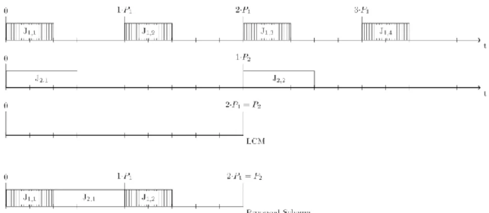
When scheduling offline, all jobs need to be pre-set on a repeating cycle that will be repeated infinitely. The cycles length needs to equal the length of the least common multiplier (LCM). For now, just think of the LCM as the length of the cycle in which all the jobs are to be accommodated on. LCM will be further explained in the next section. The repeating cycle always stretches from zero to LCM. An example of this is illustrated on where LCM is equal to 2 ∗ 𝑃1 or 𝑃2. The fourth horizontal line in proposes a schedule

where the two different jobs are scheduled. Thus far the schedule only handles the constraints of not being executed parallel to one another and being repeated as many number of times as required, according to each jobs period and with respect to LCM.

Least Common Multiplier

Each unique job has a period 𝑃𝑖 and to be able to correctly place all jobs within a repeating cycle, the

cycle needs to consist of as many time units as the LCM-value. This is illustrated in . The first and the second horizontal line represent two separate jobs that are repeated an infinite number of times. Depending on how scheduling between zero and 2 ∗ 𝑃1 or 𝑃2 is done, the same job-sequence should

repeat itself between 𝑃2 and 2 ∗ 𝑃2 and so on. Because of this there only needs to be two instances of 𝐽1,𝑗

and one instance of 𝐽2,𝑗 when constructing a schedule.

Figure 2: Timeline, LCM and proposed schedule

Interval and deadline

A job can occur multiple times over a repeating cycle. Looking at an example where job 𝐽𝑖 has a period

𝑃𝑖 = 𝐿𝐶𝑀

2 the conclusion is that it needs to be repeated two times. And therefore, two job instances,

𝐽𝑖,1 and 𝐽𝑖,2, would need to be placed within two different intervals. These are 𝐼𝑖,1 and 𝐼𝑖,2. The intervals

represent the earliest and the latest time for when a job instance needs to be executed. For instance, 𝐼𝑖,𝑗=

0,10 means that 𝐽𝑖,𝑗 has the release time 0 and the deadline 10.

The deadline of job instance 𝐽𝑖,𝑗 is denoted by 𝐷𝑖,𝑗. This can be seen in Figure 3. Each instance of 𝐽1,𝑗 can

(14)

WCET

WCET shows how long it takes, in worst case, for the job to be executed. Each job instance 𝐽𝑖,𝑗 has an

execution time of 𝑒𝑖 time units. Usually the execution time 𝑒𝑖 is presumed to be within the range of

[𝑒𝑖−, 𝑒𝑖+] where 𝑒𝑖− is the minimum execution time and 𝑒𝑖+is the maximum execution time. In this report

will only the maximum execution time be considered and notated as 𝑒𝑖. This is also illustrated in Figure 3

where each of the three instances drawn have a WCET of 𝑒1.

Figure 3: Deadline, WCET

2.1.4 Dependencies between jobs

Below are the dependencies that exist between jobs for the problem according to Arcticus, (2017).

Predecessor, trigger dependency

The trigger dependencies form a relation 𝑇𝑟𝑖𝑔𝑖= {(𝑖, 𝑗)| 𝐽𝑖is a trig predecessor for 𝐽𝑗}. A trig

predecessor must be within the same interval and executed before its successor. In other words, a job instance 𝐽𝑖,𝑗of job 𝐽𝑖 that has a trig predecessor 𝐽𝑚,𝑛 must be scheduled after 𝐽𝑚,𝑛 in every interval.

Observe that only jobs where 𝑃𝑖 = 𝑃𝑚 can have trig dependencies. This can be seen in the proposed

schedule in Figure 4. Here 𝐽2,1 is a trig predecessor to 𝐽3,1 and therefore, 𝐽2,1 must be executed before 𝐽3,1.

Predecessor, data dependency

Data can be propagated through a chain of jobs and therefore there can also exist data dependencies between jobs. The data predecessor dependencies represent all the jobs that the current job is gathering its data from. In contrast to triggers, a data dependency is a soft requirement meaning a job can be executed without necessarily receiving any data from its data predecessor. The data dependencies form a relation 𝐷𝑎𝑡𝑎𝑖 = {(𝑖, 𝑗) | 𝐽𝑖 is a data predecessor for 𝐽𝑗}. Each job instance inherits these relations from its job.

(15)

2.1.5 Placing jobs in the schedule

Below show what constraints must be met for a schedule to be considered valid according to Arcticus (2017).

Valid Schedule

The schedule is considered valid if each job is placed within its period, is not executed in parallel with another job and has its deadlines and trigger relations fulfilled. An example of this can be seen in Figure 5. The first job has two instances within the repeating cycle whereas the second and the third job only has one instance. The first job has its deadline early meaning it must be placed first. Then the second job must be placed after the first instance of the first job because otherwise it would not meet its deadline. The third job has its deadline equal to its period meaning it can be executed any time during its period-instance as long as it is after the second job.

Time of Execution

𝑇𝑖,𝑗 is the time when job 𝑖 is starting its execution for the job instance 𝑗. If a job is placed within the

repeating cycle it starts with a time of execution 𝑇𝑖,𝑗 and ends at 𝑇𝑖,𝑗+ 𝑒𝑖. Which can be seen in Figure 5.

Figure 5: Deadlines, WCET and dependencies

2.1.6 Data latency and jitter

According to Arcticus, (2017) the two properties jitter and data latency, which both depend on the schedule design, are suitable for evaluating how good a schedule is.

Data latency

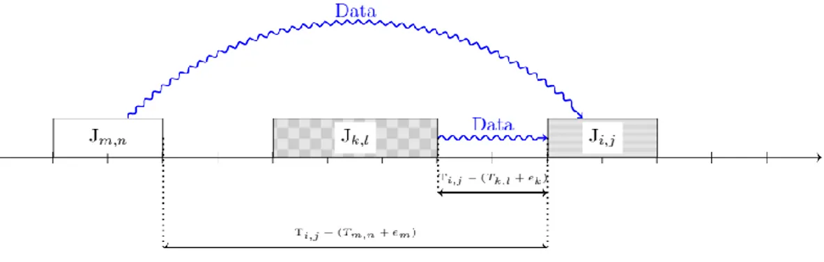
Consider two jobs 𝐽𝑖 and 𝐽𝑘 such that there is a data dependency from 𝐽𝑘 to 𝐽𝑖, (𝑘, 𝑖) ∈ 𝐷𝑎𝑡𝑎𝑖. The

immediate predecessor instance to a job instance 𝐽𝑖,𝑗 is an instance 𝐽𝑘,𝑙 such that 𝑇𝑘,𝑙+ 𝑒𝑘 < 𝑇𝑖,𝑗 and no

other instance of 𝐽𝑖 or 𝐽𝑘 will finish between 𝐽𝑘,𝑙 and 𝐽𝑖,𝑗. Let 𝐼𝑃𝑖,𝑗 be the set of all immediate data

predecessors to the instance 𝐽𝑖,𝑗. Then the data latency of each job instance 𝐽𝑖,𝑗 is 𝐿𝑖,𝑗= ∑𝐽𝑘,𝑙∈𝐼𝑃𝑖,𝑗(𝑇𝑖,𝑗−

(16)

Figure 6: Data latency

A phenomenon that comes with calculating data latency are called over- and under sampling. This is shown in Figure 7 which highlights the concept of under sampling. A job that has a data predecessor with smaller period will be executed several times, during different intervals, before the job with larger period is executed once. Only the data predecessor that is the closest to the job is of significance when

calculating the data latency.

Figure 7: Under sampling

Figure 8 shows the second example, highlighting the concept of over sampling. In this example, a job that has a data predecessor with higher period will be executed once, during different intervals, whereas the job with the lower period is executed several times. Only the data predecessor that is the closest to the job is of significance when calculating the data latency.

Figure 8: Over sampling

Going back to the example with the brakes. A minimized latency would improve the responsiveness of the system to external events, such as pressing the pedal. Therefore minimizing data latency is interesting from the perspective of how effective the system is. This is a great incentive for wanting to reduce the total data latency according to (Liu, 2000).

(17)

Jitter

By calculating the largest difference between the job instances in terms of time of execution, 𝑇𝑖,𝑗 relative

to the each period, we retrieve 𝐺𝑖 = ma x(𝑇𝑖,𝑗− (𝑗 − 1) ∗ 𝑃𝑖) – min (𝑇𝑖,𝑗− (𝑗 − 1) ∗ 𝑃𝑖) for each job

where 𝑗 = 1, … ,𝐿𝐶𝑀

𝑃𝑖 . This means that jitter is an entity which can be derived from looking at each job’s

irregularity, when comparing job instances, in execution time over the whole repeating cycle. Assume that a job 𝐽𝑖 has three instances under the whole repeating cycle. The total jitter for this job is shown in

Figure 9 as 𝐺1. Here the comparison is made between all instances of a job.

Figure 9: Jitter

In some systems, it is necessary to keep this variation between jobs small so that the system regularly produces outputs at specific time instants. Furthermore, measuring the total jitter and keeping it

(18)

2.2 OPTIMIZATION IN REAL-TIME SYSTEMS

This chapter will define optimality in real-time systems. When is a scheduler or a schedule optimal? It will also mention some commonly used algorithms for creating schedules for real-time systems.

2.2.1 Scheduler and schedules/schedule

J. W. S. Liu, (2000) states that when assigning jobs to a processor, a scheduler is acting in accordance to an algorithm that places jobs in sequences, which are called schedules, or a schedule if the scheduler only produces one job-sequence. The case for this report will be to find one job-sequence for a set of jobs and therefore the term schedule will be used here on out. Subsequently, when talking about optimality within the subject of real-time systems the aim of focus can be on either the scheduler or the schedule that the scheduler produces.

2.2.2 Scheduler optimality

Since a schedule can consist of a range of different sequences it is important that a scheduler finds a feasible solution for a set of jobs, if there is one. Therefore J. W. S. Liu, (2000) states that a scheduler is optimal if the scheduler always finds a feasible solution, or valid schedule, if there is one for the set of jobs.

In the continuation of this report the scheduler will be assumed to be optimal if nothing else is noted. The reason for why the scheduler must be optimal is because the product, Rubus®, is applied to systems where safety is of high importance. That is, it must have a valid schedule.

2.2.3 Schedule optimality

When discussing optimality for a schedule, J. W. S. Liu, (2000) states that there are not any widely adopted performance measure for schedule optimality. Real-time systems can be applied to a variety of applications and therefore there can be different aspects you want to reduce or boost, performance wise. J. W. S. Liu, (2000) mention some frequently used performance measures such as data latency, jitter, lateness, miss rate, loss rate and invalid-rate which all have their usage within different types of real-time systems.

As discussed earlier, minimizing latency improves the responsiveness of a system to external events and minimizing jitter makes sure that outputs are being produced regularly at specific time instants. The scope of this report only covers minimizing data latency but at the same time measuring to see how jitter is affected.

2.2.4 Algorithms for scheduling in real-time systems

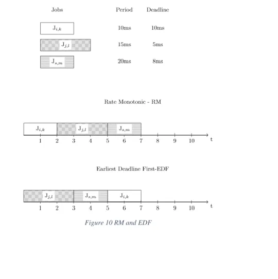
J. W. S. Liu, (2000) explains that when creating a scheduling algorithm in real-time systems, it is conventional to prioritize jobs in the order in which they should be placed. This is called priority-driven scheduling. Some of the most widely adopted scheduling algorithms for priority-driven scheduling are Rate Monotonic (RM) and Earliest Deadline First (EDF).

According to J. W. S. Liu, (2000), an assumption when regarding the optimality of RM and EDF is that all jobs need to be independent and that there are no aperiodic or sporadic jobs. As mentioned earlier, the jobs defined in this report fulfil the latter criteria but the jobs are both trigger- and data dependent. Nevertheless, RM and EDF will still lay the foundation of pillar for how to optimize the schedule. How RM and EDF are implemented in the algorithms will be explained in chapter 4.

(19)

Rate-Monotonic

Buttazo, (2005) explains that rate-monotonic scheduling works by scheduling the jobs based on their priority, each job has a period and the shorter the period is, the higher priority the job gets, for example 𝑝𝑟𝑖𝑜𝑟𝑖𝑡𝑦𝑖 =

1

𝑃𝑖. The jobs are then ordered in a list with respect to their priority. It is illustrated in what

order the jobs are placed on the schedule according to RM in Figure 10. If two jobs have the same priority, 1

𝑃1=

1

𝑃2, then further scheduling refinements need to be implemented to place equally prioritized

jobs, for example looking at the shortest WCET. Whichever of the job that has the highest priority will be placed first in the schedule and this will continue until all jobs are placed.

Earliest deadline first

Like RM, Earliest Deadline First (EDF) schedules with help of prioritization of the job set. Instead of prioritizing with respect to period, Buttazo, (2005), says that EDF prioritizes a given job set according to how soon it must be executed, where the job that has to be executed first has the highest priority. These are, as in the case with RM, placed in a specific order in a list with respect to priority. If 𝐷1,𝑗< 𝐷2,𝑘 then

the first job will have a higher priority and will be placed before the second job in the schedule. This is illustrated in Figure 10. Jobs that are equal in priority need further scheduling refinements in a similar way as mentioned for RM.

(20)

2.3 Optimization

/

Heuristics

With the scheduling problem defined, why do we choose to use heuristics? What is the relation between time complexity and the search space? This chapter will focus on answering the above questions to give some insight into the algorithms that are constructed for the scheduler.

2.3.1 What is combinatorial optimization?

As described by Lawler, (1976), combinatorial analysis, which combinatorial optimization derives from, studies the arrangements, groupings, orderings or selections of objects that are discrete (in contrast to continuous optimization).

Lawler, (1976) says that in the beginning, the study had its focus on the questions of “how many arrangements exists?” and “does an arrangement exist?” but thereafter, with the availability of computers, the question of “which arrangement is the best?” have taken the spotlight. This question would be considered naive without the advent of computers that can explore arrangements more than a thousand times faster than a human could ever do.

2.3.2 Time complexity

Ahuja, Magnanti, & Orlin, (1993) describe time complexity as an expression of how long it takes for an algorithm to execute its function with regards to the number of ingoing units and the character of the unit’s data. Practically, time complexity measures the rate of computational time increase as the problem size gets bigger.

Time complexity is important to keep track of since computational power is not an unlimited resource. For example, if an algorithm is to evaluate 𝑛 number of job instances and then test all the different possible sequences of job instances, it would have to look at 𝑛! different job sequences and therefore take increasingly long time to execute, but nevertheless it will find an optimal solution since it explores all the alternatives. Since the time complexity in the previous case increases proportionally to the number 𝑛, it is unreasonable to go on with the approach.

An example can be made were there are 400 ingoing units to the algorithm which would result in a search space of 400! ≈ 6.4 ∗ 10868_{different job sequences. Let us assume that each sequence takes 1}

nanosecond to evaluate. This means if a computer was to evaluate all these sequences it would take 4.0 ∗ 10852 years to iterate through the search space.

2.3.3 Search space

Search space is the space of all viable solutions, in the case of a scheduling problem a solution would be a sequence of all the jobs included in the problem as described by Burke & Kendall, (2014). The feasible search space is the set of all solutions within the search space that conforms to all conditions imposed on the jobs.

R. Liu, Agrawal, Liao, & Choudhary, (2014) state that to more effectively process the search space, the technique search space pre-processing more than often guides the heuristic in to an area of the search space that is more promising. According to R. Liu et al., (2014) Search space pre-processing consists of five different concepts whereas two concepts are important for this report. These are:

1. Search order reduction orders the variables in a list according to their influence on the objective function or alternatively some other condition, an example in our context are the trig

(21)

2. Search domain reduction reduces the variables’ domain to further reduce the search space, an example of this is restricting a job to a bucket where the domain for the variable Time of Execution 𝑇𝑖,𝑗 is reduced to the job interval instead of the whole length of the repeating cycle.

An example could be the domain reduction of the variable Time of Execution 𝑇𝑖,𝑗, below we can

see how the “search space” for 𝑇𝑖,𝑗 is being reduced:

Ii,j = [Pi⋅ (j − 1), . . , Pi⋅ j] This is the interval in which a job instance can be placed

𝑅𝐶 = [1, . . , 𝐿𝐶𝑀] RC is the repeating cycle (or the schedule) Ii,j ⊆ 𝑅𝐶 This means that the interval is a subset of RC

𝑇𝑖,𝑗∈ Ii,j The job instance must be executed within the interval

This is quite logical since options that would lead to invalid schedules should not even be

considered. Remember that the time of execution must be within a certain time interval otherwise it would result in an invalid schedule. That is, if any 𝑇𝑖,𝑗 ∉ Ii,j the schedule would become invalid.

An example of this could be a job with the following parameters: 𝐼𝑖,𝑗= [1,2, … ,499,500]

𝑅𝐶 = [1,2, . . . ,1999,2000]

We see that 𝐼𝑖,𝑗 ⊂ 𝑅𝐶 and the variable time of execution 𝑇𝑖,𝑗 is not confined to any set of integers

and therefore can take any integer value possible. To not test every possible integer value, domain reduction for the variable is preferable. That is, instead of letting 𝑇𝑖,𝑗 ∈ 𝑅𝐶 we reduce the domain

of 𝑇𝑖,𝑗 so that 𝑇𝑖,𝑗∈ 𝐼𝑖,𝑗.

2.3.4 Heuristics

According to Lundgren, Rönnqvist & Värbrand, (2010), methods of optimization are classified by if they are guaranteed to find an optimal solution to a presented problem or not. If the method does not always find the optimal solution to the problem, it is called a non-optimizing method and often called a heuristic. This loose definition of a heuristic means that a heuristic can be designed by very simple rules or

advanced optimization.

So why use a heuristic as solution method and have the risk to receive a non-optimal result? According to Lundgren et al., (2010), it is due to that an optimizing method often comes with some unwanted side effects, such as a long computational time and a lot of memory allocation. In contrast to optimizing methods, heuristic can avoid these side effects.

There are many classifications of heuristics, some of the more frequently used are approximation

algorithms, constructive heuristics, local search methods and metaheuristics. Whereas the latter three will be further explained because of their importance for this project.

(22)

Network design

A network’s building blocks are the edges and nodes which constitutes the graph, 𝐺 = (𝑁, 𝐵) where G is the graph that consists of nodes from the set of nodes 𝑁 and edges from the set of edges 𝐵.

Lundgren et al., (2010) explains that many problems are of the nature that make them intuitive to illustrate as a network built up on nodes and edges. Some examples of these problems are traffic networks, computer networks and telecommunication networks. By representing the problem as a network, the understanding of the problem is often increased, and solution methods can more easily be developed.

An edge can either be directed, where it has a distinct start node and end node, or undirected where the flow can go in both directions.

Combinatorial formulation

Lundgren et al., (2010) claims that for some types of heuristics one does not need to explicitly define the problem in terms of variable definitions, constraints and objective function. This is because a

combinatorial problem can for example be represented by a network, and have parts of the problem definition implicitly built in. By constructing the problem with a combinatorial formulation several of the variables, objective function and constraints do not need to be defined.

Constructive heuristics

There are many ways in which a heuristic can be initiated, every decision variable may have been given a random value within its domain, set to a predetermined value or left completely free, which means no value has been assigned to it.

According to Lundgren et al., (2010) a constructive heuristic works by initially having all its decision variables set as free and successively assigning values to them. The assignment of values works in iterations and in a way that assures a feasible solution when all variables are set.

Lundgren et al., (2010) mentions that a common type of constructive heuristic is the greedy-heuristic which works by assigning a variable a value that leads to both feasibility and effects the objective value in the most profitable way. Since the greedy-algorithm only look at the influence from its current decision variable it tends to steer the solution to non-optimality. There are many heuristics that are greedy, such as nearest neighbour and nearest addition (These heuristics are used for solving one of the most famous optimization problem, namely the traveling salesman problem.).

Local search

Lundgren et al., (2010) explains that when a feasible solution is achieved it can often be improved. The local search heuristic works by iteratively improving an already feasible solution. In each iteration, a solution 𝒙 have a set of neighbouring solutions 𝑁(𝒙) that is called the neighbourhood. What a neighbour in the set 𝑁(𝒙) is depends on the kind of decision variable, if the variable would be continuous, it can be expected to evaluate a specific range. But if it is combinatorial problem, the set 𝑁(𝒙), typically contains all solutions which can be reached by a swap. To choose an appropriate neighbourhood is one of the most important decisions when designing a local search.

Lundgren et al., (2010) also mentions that each solution 𝒚 ∈ 𝑁(𝒙) in combinatorial problems is a change of solution, this swap is dependent on what type of combinatorial problem it is. In other words, a swap

(23)

can be a change of order in each sequence or inclusion/exclusion in a problem where the decision variable is binary.

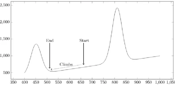
When looking into the scope of local search and optimization, local search can be described as a hill climbing heuristic. Russel & Norvig, (2010) describes the hill climbing heuristic with the mental metaphor “This resembles trying to find the top of Mount Everest in a thick fog while suffering from amnesia”. Breaking the metaphor down, the algorithm is moving in a direction that match the objective which can either be ascend or descend. The algorithm holds no memory in terms of what solutions it has visited beforehand, only the current solution. And it decides its direction depending on which

neighbouring solution holds the best value for its goal function. The algorithm will thus stop when it has reached a point where all neighbouring solutions holds values for the goal function that are worse than its current. This point is called an extrema, or local optima, which is either the maxima or minima for any given function.

Depending on the goal function the algorithm will either be searching for lower values or higher values. If the algorithm is trying to minimize a given goal function it will descend as much as possible and follow the steepest descent. If it on the other hand wants to maximize a given goal function it will follow the steepest ascent.

Figure 11 shows how the algorithm will descend until it reaches a solution that is the best when

comparing its current solution to neighbouring solutions. The Figure also presents a drawback associated with hill-climbing, the way hill-climbing is choosing its succeeding solution makes it prone to getting stuck in local extremums. This can be seen in the Figure where the algorithm gets a start solution and traverse to an end solution.

Figure 11 Hill Climbing, steepest descent

(24)

Figure 12: Pseudocode for local search

Metaheuristics

Meta is the greek word for upper level and the metaheuristic is a heuristic which stands above other heuristics. According to Du & Swamy, (2016a) the metaheuristic guides the design for other heuristics. The advantage of metaheuristics is that the lower-level heuristic can change design between iteration so that for example a start position in a local search can vary.

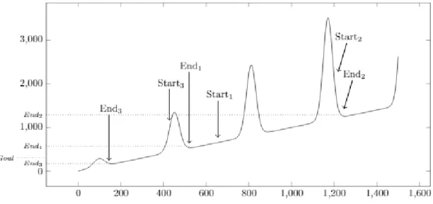
When looking at the previous example from Figure 11 it is not clear if the final end-solution is the best solution or perhaps do not reach a given goal. Therefore randomizing the start-solution, a number of times, and letting the hill-climbing algorithm find the best end-solution from each start-solution, is a viable tactic when trying to improve the goal function or reach a given goal. Russel & Norvig, (2010) describes this method as “if at first you don’t succeed, try again”. This approach can be seen in the example of Figure 13 where a goal has been set before the metaheuristic is initiated. The algorithm random-restart hill climbing initiates thereafter iterations of hill-climb search with different start-solutions until it has found an end-solution with a goal function value lower than the given goal.

(25)

Simulated annealing

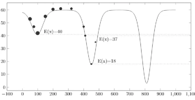
Simulated annealing is a metaheuristic which is an extension of local search. Du & Swamy, (2016) describes simulated annealing (SA) as an algorithm used to escape local minima which are not global minima. This is done by occasionally taking risks and accepting solutions that are worse than the current solution. This method tries to improve on local search so that the solution does not get stuck in local minima. A good example of this is “hill climbing” which was described earlier.

Du & Swamy, (2016) further explains that the probability of solution change, 𝑃 = 𝑒−ΔE𝑇 _{, is the factor that}

shows with what probability an inferior solution will be chosen. ΔE describes the change of the objective function between two different solution. 𝑇 is a parameter that starts with a large value and decreases after each iteration that the algorithm performs. The purpose of this is to lower the probability of changing to an inferior solution. When 𝑇 is large the probability of changing solution is high, and it is the opposite for when 𝑇 is low. The algorithm will continue running until a threshold level is met, this level is represented by parameter A.

Figure 14 Simulated annealing

Below, Figure 15, shows the algorithm for SA, according to Du & Swamy, (2016):

(26)

(27)

3 P

ROBLEM FORMULATION

The purpose of this chapter is to formulate the problem in a way so that it can be translated into a mathematical problem. The jobs will first be described as nodes and nodes that have similar properties will be grouped into buckets.

3.1 HOW THE DIFFERENT JOBS ARE TRANSLATED TO NODES

Each job instance is referred to as a node with different attributes such as WCET, deadline, period and interval. In other words, if you choose a node, all the information about a job will be revealed with the attributes mentioned above. The data- and trigger dependencies that are between nodes are represented by edges between them. The edge is either straight (trigger) or wavy (data). Free nodes are those nodes that neither have trig predecessors nor is a trig successor to any other node. Also, important to point out is that each node knows exactly how it is related to all the other nodes with regards to dependencies. Figure 16 illustrates all the above for one node.

Figure 16: Job representation with nodes

3.2 NODES GROUPED IN BUCKETS

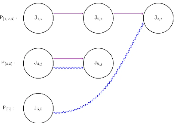
The nodes are grouped according to different periodicities. When creating the repeated cycle, with respect to the different periodicities that exist and LCM, the nodes are assigned to an interval. The nodes that belong to the same interval can further be grouped into “buckets”. Figure 17 shows six unique jobs that are grouped according to different periodicities and how they are related to one another by dependencies. In this example 𝑃1 = 𝑃2 = 𝑃3 = 15𝑚𝑠, 𝑃4 = 𝑃5 = 30𝑚𝑠 and 𝑃6 = 60𝑚𝑠. This will later be used to divide them into different buckets.

(28)

Figure 17: Example of how jobs are divided into different periodicities and how they can be related with regards to dependencies

Figure 18 shows how the jobs and how their instances are divided into different buckets. That 𝐿𝐶𝑀 = 𝑃6

means that all the nodes below are going to be scheduled in a timeline between zero and 𝑃6. 𝐽1, 𝐽2 and

𝐽3 will be scheduled four times, each in accordance with their job instance, meaning for example that 𝐽1,1,

𝐽2,1 and 𝐽3,1can only be placed between zero and 𝑃1. The remaining jobs, 𝐽4 and 𝐽5 will only be scheduled

twice while 𝐽6 will only be scheduled once. In other words, if a schedule were to be created with the jobs

represented in Figure 17 then all the nodes in Figure 18 should be scheduled with respect to their different constraint such as period, deadlines and trigger dependencies.

Figure 18 also displays how a data predecessor will create multiple arrows to all instances of a job where data will be “sent” to. To give an example, in Figure 17 𝐽₆ is a data predecessor to 𝐽3. This will result in

four arrows coming from 𝐽6 to all four instances of 𝐽3 meaning it is the data predecessor of all these

nodes. Later, depending on where 𝐽6,1 is placed in the schedule only the arrow closest to the first instance

of 𝐽3,𝑗 will be measured when calculating data latency. (This is an example of under sampling.)

Figure 18: Buckets and how the jobs extend to nodes

Earlier it was also mentioned that a schedule will be repeated an infinite number of times. Because of this, some nodes that are executed towards the end of the cycle could send its data "backwards". This is shown in Figure 18 as the dotted arrow from 𝐽4,2 to 𝐽5,1.

(29)

3.3 THE SCHEDULE

The schedule will now be represented by a repeated cycle. The cycle consists of 𝐿𝐶𝑀 numbers of units and the starting time is 0. A node will occupy 𝑊𝐶𝐸𝑇 number of units when it is placed on the schedule, this is where the node will be executed as well. For a schedule to be considered valid, these requirements need to be fulfilled:

 All nodes need to be placed within the cycle of the bucket in which they are placed in.  All trigger dependencies and deadlines must be met.

To minimize the data latency, the nodes with data dependencies need to be placed as close to each other as possible, without interfering with the requirements for a valid schedule. Jitter will be minimized if all nodes are placed at the same place relative to the start of their bucket.

3.4 THE NEIGHBOURHOOD

When looking at the neighbouring solutions for a specific node, the set of possible swaps with another node are the swaps which would result in a valid schedule.

3.5 EVALUATION MEASURES

As can be seen, if there are many jobs, the time complexity rises quite quickly and therefore it is of great importance that a schedule is created with a low time complexity. This means that when the number of jobs is increased, the computational time for the algorithm should not increase too much. At the same time, we will evaluate whether the algorithm is minimizing data latency and making sure that all the jobs are placed in an acceptable order with regards to period, deadline and triggers so that the schedule becomes viable. To summarize it, the points below will be used to evaluate the algorithms in chapter 4:

 The time it takes for scheduling a valid job sequence  Accumulated data latency and jitter between jobs

Data latency and jitter are two separate entities with different levels of importance. In this report focus will only be on satisfying the customers of Arcticus. Arcticus has expressed themselves that data latency is the factor that weighs in more when considering customer satisfaction, but they still want to minimize jitter. Therefore, the focus will solely be on reducing the data latency and later looking at how jitter is affected.

(30)

(31)

4 T

HE THREE ALGORITHMS THAT HAVE BEEN STUDIED

The three different schedulers are implemented by three different algorithms which are placed relative one another on the horizontal line illustrated below. This means that algorithm 1, which is placed the furthest to the left, will have a smaller search space to work on compared to the other algorithms. This in turn means that a solution will be generated faster than algorithm 2 and algorithm 3 but the solution will probably be worse. The search space expands the further you move right on the line which means that algorithm 3 will produce the best solution but it will also take more time to compute. This is the premise for the three algorithms that will be presented in this chapter.

Figure 19 Search space impact

4.1 GREEDY CONSTRUCTIVE ALGORITHM

The first algorithm will be based on the algorithms RM and EDF from real-time schedulers, with some tweaks to make sure that the schedule remains valid. This algorithm will find a valid schedule as fast as it can and it is a greedy constructive algorithm. Referring to the horizontal line it is placed to the left meaning focus will be on creating a job sequence with low time complexity. This algorithm will not consider the data dependencies at all.

4.1.1 Keeping schedule valid

The trick used for the greedy constructive algorithm, and the remaining two algorithms, is finding a critical path which is further explained in section 4.1.2.This ensures that the schedule remains valid. To find the critical path, all nodes are first placed into different buckets. The bucket order refers to how RM works, taking all jobs with lower periods first. Then each bucket, which consist of nodes, will rearrange the order of the nodes with accordance to the critical path and with respect to trigger dependencies and deadlines as mentioned before.

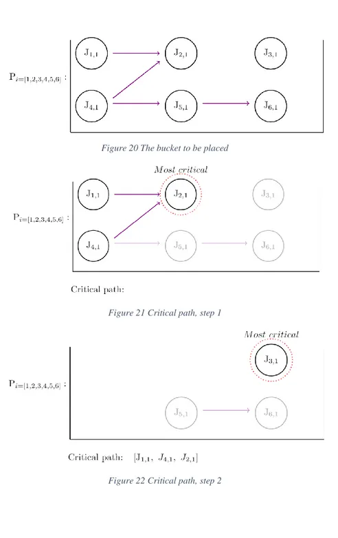
4.1.2 Critical path

Figure 20 to Figure 24 illustrates how a critical path is chosen. By looking at all the nodes in a specific bucket, the algorithm will sort the nodes according to deadlines and trigger dependencies. This will ensure that the nodes will have their precedence constraint and deadline fulfilled. The shortest deadline for a node is determined by how soon it must be executed in the schedule. A node with earlier deadline will therefore always be executed before a node with a later deadline. If a node has a deadline and trig predecessors, then the node predecessors will have their deadlines updated in a way so that there is enough time for the node successor to be executed. In this case assume that node 𝐽{2,1} is the most critical

node, with respect to deadline and the number of nodes that must be placed before it. Because node two has node one and node four as trig predecessors these nodes must be placed before node two, an

illustration of the pick can be seen in Figure 21. Whether node one or four will be placed first is based on chance, in this case number one is smaller than number four and the algorithm will sort accordingly. Next, assume that node 𝐽{3,1} and 𝐽{6,1} are equal in criticality. Since three is smaller than six it will be placed

(32)

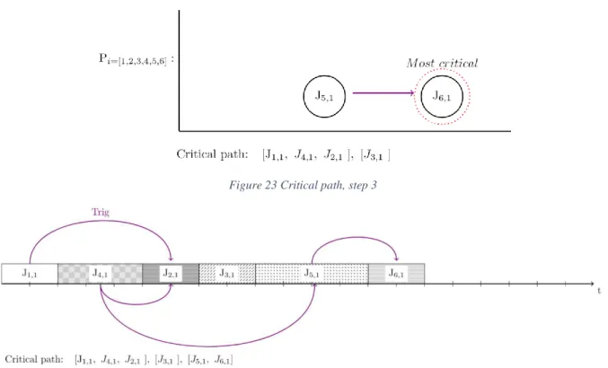
second, this step can be seen in Figure 22. After node 3 has been sequenced node 6 can be picked which gets illustrated in Figure 23. The sequence for the complete critical path is shown in Figure 24.

Figure 20 The bucket to be placed

Figure 21 Critical path, step 1

(33)

Figure 23 Critical path, step 3

Figure 24: Critical path, final placement

4.1.3 Bucket order

Figure 25 shows how five different jobs are first placed in three different buckets. The smaller buckets have a period of 𝑃[1,2,3] = 10 milliseconds and the bigger bucket has a period of 𝑃[4,5]=

20 milliseconds = 𝐿𝐶𝑀. Secondly the nodes are sorted according to the critical path in each bucket and Figure 25 shows in what order the buckets will be propagated in the schedule, were bucket 1 will be placed first, bucket 2 second and bucket 3 lastly.

Figure 25: Bucket order

4.1.4 Iteration through buckets

In Figure 26 it is illustrated how the jobs are placed according to the critical path and the ordering of the bucket placement. In iteration 1, all the jobs from the first bucket are placed on the timeline. In iteration 2 all the jobs from the second bucket are placed. These are not placed under the same interval even though

(34)

there is room for it because each job must be repeated every period. In iteration 3 the third bucket is placed with node four and five.

Figure 26: Iteration through buckets

4.1.5 Pseudocode for greedy constructive algorithm

Figure 27: Pseudocode for greedy constructive algorithm

The algorithm starts by creating the schedule with LCM number of units. Each unit represent one unit of execution time for the jobs. Then all the nodes are grouped into different buckets. The buckets are placed in a list called “Allbuckets” in the order in which they will be evaluated. Lastly each bucket will sort their nodes according to the critical path and then the jobs will be placed on the schedule.

4.2 LOCAL SEARCH ALGORITHM

The second algorithm will mimic the greedy heuristic used in section 4.1 but with an extra tweak. It will take data dependency fulfilment into account when placing jobs during the greedy construction of the schedule. The algorithm will also be extended to local search meaning after a schedule is created, the algorithm will consider to change order of the jobs if this leads to a lower objective value.

(35)

4.2.1 Minimizing the data latency

During each iteration of the greedy construction of the schedule, it will evaluate where the best placement for the node is when it is to be placed. The algorithm here is the same as for the greedy constructive algorithm when finding the critical path. But instead of just placing the node after the last placed node, it will evaluate placing the nodes in-between other nodes. The evaluation of spots in-between jobs is thus purely a greedy heuristic. For details, see 4.2.2.

Later, after the schedule has been created, a new evaluation will be made. This is a rearrangement of the nodes already placed and can be referred to as a local search. Each time when evaluating a neighbouring solution, the total data latency will be measured and compared to the earlier total data latency. If there is a better solution the algorithm will keep rearranging the nodes.

4.2.2 Evaluation of spots in-between jobs

Figure 28presents the idea of scheduling jobs in-between jobs that are already scheduled. The situation that is described is the placement of 𝐽6,𝑜. The arrows below the cycle shows all possible placements due to

the latest trig dependency for 𝐽6,𝑜. These arrows are the different candidate-placements for the job. Each

arrow will be evaluated to find an optimal placement with respect to data dependencies when the

algorithm decided to place 𝐽6,𝑜 on the schedule. Simultaneously, evaluation regarding other jobs deadlines

will be taken into consideration so that the schedule remains valid. If the validity of the schedule is not affected, then “candidate 1” is the best possible placement in this example.

Figure 28: Evaluation of spots in-between jobs

4.2.3 Rearrangement of jobs after completion of schedule

Figure 29illustrates how the heuristic technique local search is used after a schedule is created. The upper cycle is an example of a schedule where all the jobs have been placed. The idea is that all the smaller buckets will be rearranged, if possible, to minimize the total data latency. Within each bucket, each node’s neighborhood will get evaluated and changed to, if a neighboring solution is preferable to the current. When creating a neighborhood the trick is to create a span, lower and upper bound, in which the node can be placed within, without making the schedule invalid. The arrows in Figure 29, above the “candidate 1” and “candidate 4”, represent the lower- and upper bound for 𝐽_6,𝑜.

(36)

Figure 29: Rearrangement of jobs in buckets after schedule is created

4.2.4 Pseudocode for local search algorithm

(37)

The local search algorithm works exactly as the greedy constructive algorithm until step 11. Instead of just placing the nodes according to the critical path, this algorithm will first find all possible spots for a node to be placed on. The placement is then done by first identifying which of the candidates that lead to the minimum increase in data latency and thereafter place it at the same candidate position, this is further explained in section 4.2.2. After a schedule has been produced the schedule will try to further reduce its data latency by rearranging the nodes in the schedule.

In Figure 30, at step 23 the procedure LocalSearch is presented. The procedure goes through the

schedule’s buckets and tries to find better placements for each node by identifying the neighborhood of a node and picks the best solution.

4.3 SIMULATED ANNEALING

The third algorithm will be based on the principles of the local search algorithm but extended into Simulated annealing (SA). This algorithm does not have the same time constraint and can therefore more thoroughly explore job sequences and find a solution that is better. This algorithm is placed to the right relative to the other ones on the horizontal line in chapter 4, Figure 19.

4.3.1 Initial solution

The initial solution that the SA algorithm will try to improve will be produced by local search algorithm. This initial solution will act as the starting point from which the SA algorithm will further explore the neighbouring solutions.

4.3.2 Evaluation and placement of jobs

Like the second algorithm, SA will iterate through each neighbouring solution and evaluate how the total data latency would change in each possible placement. If there is a swap which would lead to a clear improvement for the current solution, the swap will be executed. But if the current solution is proved to be the best solution, regarding the total data latency, no swap would lead to an improvement. However, in the SA algorithm there is a probability that there will be a swap anyway and that it will lead to a higher total data latency value.

The difference here from the second algorithm is that a job, when there are no good rearrangements, can still make the switch with another job with a certain probability. This probability is decreasing after each iteration meaning that eventually the algorithm will behave like the local search algorithm.

An illustrative explanation of these two scenarios can be seen in Figure 31 and Figure 32. When going through the first scenario in Figure 31 it can be seen that 𝐽6,𝑜’s neighbourhood consists of the potential

swaps [candidate 1, candidate 2, candidate 3] and that a swap with either candidate 1 or candidate 2 will improve the data latency which gets incurred by 𝐽6,𝑜’s data dependencies. The most beneficial swap in

(38)

Figure 31 Placement with SA when there is clear improvement

When looking at the other scenario in Figure 32 it can be seen that 𝐽6,𝑜’s neighbourhood consists of the

potential swaps [candidate 1, candidate 2, candidate 3] but there is not any clear improvement and if the algorithm were to make a greedy decision it would be to choose candidate 1, that is not to swap at all. In the case with the SA algorithm there is still a chance that there would be a swap that would lead to a higher data latency.

Figure 32 Placement with SA when there is no clear improvement

4.3.3 Benefits of making non-greedy job rearrangements

The purpose of SA is to explore job-sequences that are not being evaluated in the earlier algorithms. This will make sure that the search space is larger with the possibility of ending up with a lower objective value. Only schedules with lower objective value will be saved throughout the algorithm. An example of this can be seen in Figure 33 where 𝐽3,𝑙 is placed directly after its preceding trigger dependency and in

front of its succeeding trigger dependency, that is, when computing the neighborhood for 𝐽3,𝑙 it will only

get one candidate, its current position. When looking at 𝐽6,𝑜 in Figure 34 the job has swapped place in the

sequence, even though it does not give any direct reduction in data latency for the solution. What it has done though is to have expanded the neighborhood for 𝐽3,𝑙.

(39)

Figure 33 locked job-position

(40)

4.3.4 Pseudocode for SA algorithm

Figure 35: Pseudocode for SA algorithm

This algorithm works exactly as the local search algorithm until step 33. Then a parameter called P is introduced. The purpose of P is that when rearranging nodes, there can sometimes be switches between nodes that result in a higher total data latency. This switch will be made with a probability of P and the probability P is decreasing after each iteration. This can be seen at Step 44. If the best-found spot is equal to the former spot meaning, there is no switch that is beneficial for minimizing the objective value then the algorithm will still make a switch with the probability P. This will loop until all jobs in the schedule have been evaluated and until P is very low.

(41)

5 R

ESULT

In this chapter, the different instances, with jobs that were to be scheduled, will be presented together with the results from solving these instances with the three different scheduling algorithms. The algorithms were implemented in Python 3.6.

5.1 THE INSTANCES TO BE SCHEDULED

To develop and evaluate the algorithms, three different instances was provided by Arcticus. These three scheduling instances have different challenges which makes them suitable for evaluation during algorithm development. The first two instances are mainly used to observe whether the algorithm makes smart choices or not. The third instance consist of more than 300 jobs which makes it more useful for evaluating the efficiency of the algorithms. This is referred to as “the real problem” and is described in chapter 5.1.3. One thing to keep in mind is that each time unit described from now on out equals 5𝜇s. This time unit will be described with parameter 𝑡, in other words 1𝑡 = 5𝜇s

5.1.1 Easy problem

The first instance is called “the easy problem” and consist of three jobs, see Figure 36 to see all their dependencies as well. All the three jobs have the same period length (𝑃1= 𝑃2 = 𝑃3), 𝐽1,𝑖 is a predecessor

to 𝐽2,𝑖 and 𝐽3,𝑖 is sending data to 𝐽1,𝑖.

´

Figure 36: Easy problem

5.1.2 Hard problem

The second instance is called “the hard problem” and consist of five jobs, see Figure 37 to see all their dependencies as well. The five jobs have three different period lengths i, j and k. 𝐽1,𝑖 is receiving data

from 𝐽3,𝑗,, 𝐽2,𝑖 needs to be executed after 𝐽1,𝑖, 𝐽3,𝑗 is receiving data from 𝐽5,𝑘, 𝐽5,𝑘 is receiving data from 𝐽4,𝑘

and needs to be executed after 𝐽4,𝑘.

(42)

5.1.3 The real problem

The real problem enables a more holistic benchmarking of the three algorithms. This problem’s characteristics are that it consists of 357 jobs with five different periods 5.000, 10.000, 20.000, 50.000 and 100.000 units of t which combined have a LCM of 100.000 units of t. Altogether, the 357 jobs have 2267 job instances, or nodes, which need to be scheduled.

An example of how a job is structured can be seen in Figure 38, in this specific description 𝐽275,𝑗, 𝑗 =

[1, . . , 𝐿𝐶𝑀/𝑃275] = [1, . . ,10], is described and it can be seen that 𝑊𝐶𝐸𝑇 = 𝑒275= 30𝑡, 𝑃275= 10.000𝑡

and that 𝐽275,𝑗 needs to be executed within its interval 𝐼275,𝑗 since deadline is 𝐷275,𝑗 = 0𝑡. For this

problem all deadlines are set to the end of each period, and thus resulting in a more relaxed problem. The job has fourteen data predecessors "DataDependency" and one trig successor "TrigSuccessor".

Figure 38 Structure of node data

5.2 RESULTS FROM THE ALGORITHMS

The first instance, described in Figure 36, received the following schedules and results from the three different algorithms.

5.2.1 Easy problem

Figure 39 shows the schedule created when applying the greedy constructive algorithm on the “easy problem”. We see that 𝐽1,1 is placed first, then comes 𝐽2,1 and lastly 𝐽3,1.