Elastic Anisotropy of Deformation Zones in both Seismic and Ultrasonic Frequencies: An Example from the Bergslagen Region, Eastern Sweden

Examensarbete vid Institutionen för geovetenskaper

ISSN 1650-6553 Nr 265

Elastic Anisotropy of Deformation

Zones in both Seismic and Ultrasonic

Frequencies: An Example from the

Bergslagen Region, Eastern Sweden

Elastic Anisotropy of Deformation Zones in both

Seismic and Ultrasonic Frequencies: An Example

from the Bergslagen Region, Eastern Sweden

Pouya Ahmadi

Pouya Ahmadi

Estimation of elastic anisotropy, which is usually caused by rock fabrics and mineral orientation, has an important role in exploration seismology and better understanding of crustal seismic reflections. If not properly taken care of during processing steps, it may lead to wrong interpretation or distorted seismic image. In this thesis, a state-of-the-art under the development Laser Doppler Interferometer (LDI) device is used to measure phase velocities on the surface of rock samples from a major deformation zone (Österbybruk Deformation Zone) in the Bergslagen region of eastern Sweden. Then, a general inversion code is deployed to invert measured phase velocities to obtain full elastic stiffness tensors of two samples from the major deformation zone in the study area. At the end, results are used to correct for the anisotropy effects using three dimensionless Tsvankin's parameters and a non-hyperbolic moveout equation. The resulting stacked section shows partial reflection improvement of the deformation zone compared with the isotropic processing section. This suggests that rock anisotropy may also contribute to the generation of reflections from the deformation zones in the study area but requires further investigations.

Examensarbete vid Institutionen för geovetenskaper

ISSN 1650-6553 Nr 265

Elastic Anisotropy of Deformation

Zones in both Seismic and Ultrasonic

Frequencies: An Example from the

Bergslagen Region, Eastern Sweden

Abstract

Estimation of elastic anisotropy, which is usually caused by rock fabrics and mineral orientation, has an important role in exploration seismology and better understanding of crustal seismic reflections. If not properly taken care of during processing steps, it may lead to wrong interpretation or distorted seismic image. In this thesis, a state-of-the-art under the development Laser Doppler Interferometer (LDI) device is used to measure phase velocities on the surface of rock samples from a major deformation zone (Österbybruk Deformation Zone) in the Bergslagen region of eastern Sweden. Then, a general inversion code is deployed to invert measured phase velocities to obtain full elastic stiffness tensors of two samples from the major deformation zone in the study area. At the end, results are used to correct for the anisotropy effects using three dimensionless Tsvankin's parameters and a non-hyperbolic moveout equation. The resulting stacked section shows partial reflection improvement of the deformation zone compared with the isotropic processing section. This suggests that rock anisotropy may also contribute to the generation of reflections from the deformation zones in the study area but requires further investigations.

Acknowledgements

I would like to express my deepest appreciation to all those who provided me the possibility to complete this thesis. A special gratitude I give to my supervisor, Dr. Alireza Malehmir, whose contribution in productive suggestions and encouragement, helped me to complete this thesis.

Special thanks go to my dearest friends, Taher Mazloumian, Ershad Gholamrezaie, Hanieh Shahrokhi, Amir Abdi, Omid Ahmadi, Ashkan Dorostkar and Magnus Andersson who helped me with their useful comments and suggestions about my thesis.

I have to appreciate the guidance given by other professors and supervisors especially in my project presentation that has improved my presentation skills thanks to their comments and ad-vices.

Furthermore, I would also like to thank:

• Dr. Robert W. Vestrum for letting me run his codes and use his helpful advices.

• Geological Survey of Sweden for financially supporting the Dannemora data acquisition and collecting rock samples.

• Dr. Maxim Lebedev for his corporation during laboratory measurements.

• GLOBE ClaritasT M _{under license from the Institute of Geological and Nuclear Sciences}

Limited, Lower Hutt, New Zealand was used to process the seismic data.

• This master thesis has been done in collaboration with Curtin University in Perth.

Last but not least, I would like to express my love and gratitude to my beloved family: my wife, father, mother and sister; for their understanding and endless love, through the duration of my studies.

Contents

Acknowledgements II

List of Figures V

List of Tables VI

List of Abbreviations VII

1 Introduction 1

2 Background 3

2.1 General . . . 3

2.2 Anisotropic Form of Hook's Law . . . 3

2.3 Propagation of Elastic Waves in Anisotropic Media . . . 4

2.4 Voigt Notation . . . 5

2.5 Common Anisotropy Classes . . . 6

2.6 Phase Velocities for Two Anisotropy Classes . . . 8

2.7 Thomsen's notation for weak anisotropy in TI media . . . 9

2.8 Tsvankin's extended Thomsen's parameters for orthorhombic media . . . 10

3 Laboratory Measurements 12 3.1 Laser Doppler Interferometer Device . . . 12

3.2 Inversion . . . 13

3.3 Results . . . 14

3.4 Discussion . . . 16

4 Real Seismic Data 18 4.1 Background . . . 18

4.2 From The Laboratory to the Real Data . . . 20

4.3 Results . . . 20

4.4 Discussion . . . 24

5 Conclusions 28

List of Figures

1.1 Map of the area of interest . . . 2

3.1 Laboratory Instrument and samples . . . 12

3.2 Velocity of particle motion and the hodogram . . . 13

4.1 Geological map of the study area . . . 18

4.2 CDP 1612 after applying NMO . . . 21

4.3 The unmigrated stacked section before introducing anisotropy . . . 22

4.4 The unmigrated stacked section after introducing anisotropy . . . 23

4.5 Closer look of the unmigrated stacked sections before and after . . . 24

4.6 Portions of the unmigrated stacked section before and after . . . 25

4.7 Azimuth-offset coverage of the data . . . 25

List of Tables

3.1 Input data summary . . . 14 3.2 Comparison of the results . . . 16 4.1 Acquisition parameters and processing steps of the data . . . 19

List of Abbreviations

3C Three-Component 3D Three-Dimension

ÖDZ Österbybruk Deformation Zone CDP Common-depthpoint

CMP Common-midpoint DMODip Moveout

LDI Laser Doppler Interferometer NMONormal Moveout

SGU Sveriges Geologiska Undersökning TI Transversely Isotropic

1

Introduction

The Bergslagen region, located in south-central Sweden, is a major ore producing area in Swe-den with more than 1000 years of mining history (Malehmir et al., 2011; Allen et al., 1996; Stephens et al., 2009). This part was mapped by the Geological Survey of Sweden (Stålhös, 1991) and investigated more afterward (Bergman et al., 1996; Antal et al., 1998; Juhlin and Stephens, 2006; Stephens et al., 2009). Moreover, some valuable petrophysical measurements are available for different rock types at the Geological Survey of Sweden (Stephens et al., 2009). Ongoing studies show a major deformation zone , the Österbybruk Deformation zone (ÖDZ), in the south-east part of this area (Dahlin and Sjöström, 2010).

Malehmir et al. (2013) recently investigated petrophysical properties of the major deformation zone (Österbybruk Deformation Zone) in the same area (Figure 1.1). Using a Laser Doppler Interferometer (LDI) device (Figure 3.1a, b), they suggested up to 10% velocity-anisotropy as-sociated with a major reflective package in the seismic data (Malehmir et al., 2011). The origin of the package was linked to a combination of anisotropy and amphibolite lenses within the de-formation zone (Malehmir et al., 2011, 2013). However, their seismic data processing did not account for the anisotropy and a full exploitation of the LDI measurements was not provided.

LDI device has been used in many investigations (Pouet and Rasolofosaon, 1990; Martin et al., 1994; Rasolofosaon et al., 1994; Bayón and Rasolofosaon, 1996; Nishizawa et al., 1997; Fukushima et al., 2003). Lebedev et al. (2011) introduced a new method for conducting laboratory mea-surements of P- and S-waves velocities and polarizations in rock samples using a Laser Doppler Interferometer (LDI) device. The main advantages of using LDI instead of piezoelectric trans-ducers are that (1) the area of measurement is much smaller than the wavelength and (2) the full particle velocity vector can be recorded (Lebedev et al., 2011). Using the equipment, one is able to measure particle velocities excited by a P- or S-wave transducer in a small portion of a sample along the direction of the laser beam and transform them into a 3-component (3C) particle/velocity vector (if three orthogonal measurements are done). These measurements are useful because they can provide information about the stiffness tensor especially for anisotropic rock samples that combined with the density of the material could provide a better understand-ing of elastic wave propagation within the samples.

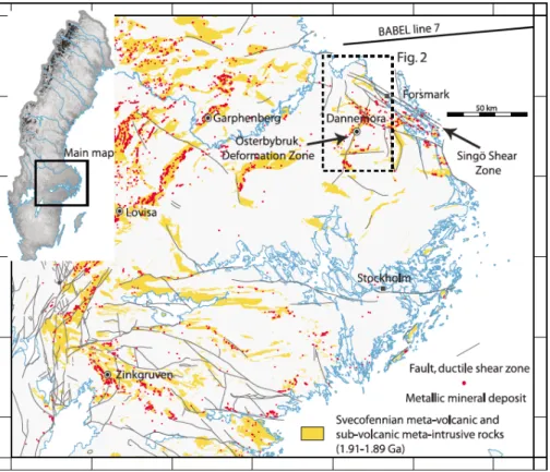
Figure 1.1: General geological map of the study area, Dannemora, in the northeastern part of the Bergslagen region. Österbybruk Deformation Zone (ÖDZ) is the main target of this study (modified from Malehmir et al., 2011).

Different experiments and theoretical investigations have been carried out on different materi-als attempting to estimate their full elastic stiffness tensor. One of the successful attempts was by Vestrum (1994), which would be briefly described in section 3.2 and his approach is used in this thesis.

The main objectives of this thesis, therefore, are:

1. To invert phase velocity data from the LDI measurements for elastic stiffness tensor with-out assuming any kind of symmetry as a priori information.

2. To include anisotropy parameters in the processing for a comparison with the original processing work (Malehmir et al., 2011). In this thesis, for example, by including some percentage of anisotropy partial improvement of the seismic image of the deformation zone is observed, which further supports the idea that the deformation zone is anisotropic to the seismic wave.

2

Background

2.1

General

Different experiments and theoretical investigations have been done on different material trying to estimate the full elastic stiffness tensor. Jech (1991), Arts (1993) and Vestrum (1994) used a generalised linear inversion method to calculate all the 21 elements. Arts (1993) and Vestrum (1994) assumed no symmetry to solve the equation for all 21 unknowns. Mah and Schmitt (2003) used almost similar method to what Vestrum used but with different input data and a slightly modified code to be more stable for their experiment setup.

Tsvankin (1997) introduced the dimensionless anisotropic parameters preserving all benefits of Thomsen's notation (Thomsen, 1986) in wave propagation for orthorhombic media which is used here to introduce anisotropy to the processing steps and in the same time link the stiffness tensor to the real seismic data which will be mentioned in section 2.8.

It should also be mentioned that all the equations and formulations used in this chapter are extracted from The Rock Physics Handbook, 2nd edition (Mavko et al., 2009). Readers are invited to see this book for detailed exploitation of the equations.

2.2

Anisotropic Form of Hook's Law

From the generalized Hook's law for anisotropic, linear and elastic media, we have the relation between stress and strain tensors:

τij = Cijklεkl, (2.1)

where τij and εklare the components of the stress and strain tensors and Cijklare the elements

of the fourth rank elastic stiffness tensor that obey the tensor transformation law and have 81 components which are not independent. The symmetry of the stress and strain tensors implies:

Cijkl= Cjikl = Cijlk = Cjilk, (2.2)

which reduces the independent constants to 36. Some thermodynamic considerations reduce the number of independent components to 21 (Arts et al., 1991), which require:

So, the total number of independent constants which a homogeneous linear elastic material can have is 21. Some symmetry considerations might imply some limitations and reduce the inde-pendent constants. The maximum symmetry (isotropic) is characterized by only two constants and the most general case (triclinic) is described by 21 constants.

2.3

Propagation of Elastic Waves in Anisotropic Media

From the Newton's second law and the definition of the strain tensor the following equation will be reached. ρ∂ 2_u i ∂t2 − Cijkl ∂2_u k ∂xi∂xj = 0, (2.4)

where u is the displacement and ρ is the density of the material. Now by considering a harmonic plane wave we have:

ui = Aiei

2π

λ(njxj−vt), (2.5)

where the plane wave propagates in the direction of a unit vector, n, normal to the wave form and Aiare the components of the amplitude of the particle displacement vector, λ is the wavelength,

xj are the components of the particle position vector, v is the phase velocity and t is the time

that the wave traveled. By rewriting (2.4) using (2.5) we will reach to the Christoffel's equation:

ΓilAl= ρv2Ai, (2.6)

Γilare the Christoffel symbols which are the components of a second order matrix that depends

on the elastic constants via:

Γil = Cijklnjnk. (2.7)

We can rewrite the Christoffel's equation to be able to use it in forward modelling an inverse problem:

(Cijklnjnl− ρv2δik)Ak = 0, (2.8)

2.4

Voigt Notation

In elasticity, it is standard and simple to use Voigt notation for stresses, strains and stiffness tensors. We can write the stresses and strains as six-element column vectors instead of nine-element square matrices;

T =             σ1 = σ11 σ2 = σ22 σ3 = σ33 σ4 = σ23 σ5 = σ13 σ6 = σ12             , E =             e1 = ε11 e2 = ε22 e3 = ε33 e4 = 2ε23 e5 = 2ε13 e6 = 2ε12             . (2.9)

In the stiffness tensor, use of Voigt notation will reduce the subscripts from 4 to 2 using the following convention: ij(kl) I(J) 11 1 22 2 33 3 23,32 4 13,31 5 12,21 6 , (2.10)

each pair of indices ij(kl) is replaced by one index I(J). So, the elastic stiffness can be written as: (CIJ) =             C11 C12 C13 C14 C15 C16 C21 C22 C23 C24 C25 C26 C31 C32 C33 C34 C35 C36 C41 C42 C43 C44 C45 C46 C51 C52 C53 C54 C55 C56 C61 C62 C63 C64 C65 C66             . (2.11)

Note that the Voigt representation of stiffness tensor is symmetric and the upper triangle con-tains 21 elements, which are needed to describe the most general case of anisotropy (triclinic).

The Hook's law using the Voigt notation is:             σ1 σ2 σ3 σ4 σ5 σ6             =             C11 C12 C13 C14 C15 C16 C21 C22 C23 C24 C25 C26 C31 C32 C33 C34 C35 C36 C41 C42 C43 C44 C45 C46 C51 C52 C53 C54 C55 C56 C61 C62 C63 C64 C65 C66                         ε1 ε2 ε3 ε4 ε5 ε6             . (2.12)

It is worth to mention that the stress and strain vectors and stiffness matrix in Voigt notation are not tensors and do not follow the laws of tensor transformation. So, we should be careful when transforming from one coordinate system to another. We can always go back to four-index notation to go between coordinate systems.

2.5

Common Anisotropy Classes

Voigt stiffness matrix structure for common anisotropy classes are:

• Isotropic: two independent constants, the most symmetric case (e.g. glass),

CIJ =             C11 C12 C12 0 0 0 C12 C11 C12 0 0 0 C12 C12 C11 0 0 0 0 0 0 C44 0 0 0 0 0 0 C44 0 0 0 0 0 0 C44             , C12 = C11− 2C44. (2.13)

• Cubic: three independent constants. This structure has three planes of symmetry (e.g. Halite, N aCl), CIJ =             C11 C12 C12 0 0 0 C12 C11 C12 0 0 0 C12 C12 C11 0 0 0 0 0 0 C44 0 0 0 0 0 0 C44 0 0 0 0 0 0 C44             . (2.14)

• Hexagonal or Transversely Isotropic (TI): five independent constants (e.g. Nepheline, N a3KAl4S4O16). This is valid when the axis of symmetry lies along the X3-axis:

CIJ =             C11 C12 C13 0 0 0 C12 C11 C13 0 0 0 C13 C13 C33 0 0 0 0 0 0 C44 0 0 0 0 0 0 C44 0 0 0 0 0 0 C66             , C12 = C11− 2C66. (2.15)

• Orthorhombic: nine independent constants (e.g. Olivine, (M g, F )2SiO4),

CIJ =             C11 C12 C13 0 0 0 C12 C22 C23 0 0 0 C13 C23 C33 0 0 0 0 0 0 C44 0 0 0 0 0 0 C55 0 0 0 0 0 0 C66             . (2.16)

• Monoclinic: 13 independent constants (e.g. Halotrichite, F eAl2(SO4)4.22H2O),

CIJ =             C11 C12 C13 0 C15 0 C12 C22 C23 0 C25 0 C13 C23 C33 0 C35 0 0 0 0 C44 0 C46 C15 C25 C35 0 C55 0 0 0 0 C46 0 C66             . (2.17)

• Triclinic: 21 independent constants, the most general case (e.g. Tantite, T a2O5),

CIJ =             C11 C12 C13 C14 C15 C16 C12 C22 C23 C24 C25 C26 C13 C23 C33 C34 C35 C36 C14 C24 C34 C44 C45 C46 C15 C25 C35 C45 C55 C56 C16 C26 C36 C46 C56 C66             . (2.18)

2.6

Phase Velocities for Two Anisotropy Classes

The phase velocities of wave propagation in isotropic media are:

VP = √ C11 ρ , VS = √ C44 ρ . (2.19)

But in anisotropic media, generally, there are three modes of propagation.

• Quasi-longitudinal (VP)

• Quasi-shear (VSV)

• Pure-shear (VSH)

For Transversely Isotropic (TI) medium in any plane containing the symmetry axis we have:

Quasi-longitudinal: VP = ( C11sin2θ + C33cos2θ + C44+ √ M )1/2 (2ρ)−1/2, (2.20) Quasi-shear: VSV = ( C11sin2θ + C33cos2θ + C44− √ M )1/2 (2ρ)−1/2, (2.21) Pure-shear: VSH = ( C66sin2θ + C44cos2θ ρ )1/2 , (2.22) where, M =[(C11− C44)sin2θ− (C33− C44)cos2θ ]2 + (C13+ C44)2sin22θ,

and θ is the angle between the wave vector and the x3-axis of symmetry (θ = 0 for propagation

along the x3-axis).

Phase velocities of three modes of propagation of an Orthorhombic medium in one of the three symmetry planes ([x1, x3] plane) are:

Quasi-longitudinal: VP = ( C55+ C11sin2θ + C33cos2θ + eA )1/2 (2ρ)−1/2, (2.23) Quasi-shear: VSV = ( C55+ C11sin2θ + C33cos2θ− eA )1/2 (2ρ)−1/2, (2.24) Pure-shear: VSH = ( C66sin2θ + C44cos2θ ρ )1/2 , (2.25) where, e

A =√(C55+ C11sin2θ + C33cos2θ)2− 4A,

A = (C11sin2θ + C55cos2θ)(C55sin2θ + C33cos2θ)− (C13+ C55)2sin2θcos2θ,

and θ is the angle of the wave vector relative to the x3-axis (θ = 0 for propagation along the

x3-axis).

2.7

Thomsen's notation for weak anisotropy in TI media

Thomsen (1986) introduced three constants along with the P- and S-wave velocities (denoted here by α and β, respectively) for TI media, which are weakly anisotropic:

α = √ C33 ρ , β = √ C44 ρ , (2.26) ϵ≡ C11− C33 2C33 , (2.27) σ ≡ (C13− C44) 2− (C 33− C44)2 2C33(C33− C44) , (2.28) γ ≡ C66− C44 2C44 . (2.29)

Using the above constants, we can approximate three phase velocities:

VP(θ) ≈ α

(

1 + σsin2θcos2θ + εsin4θ), (2.30) VSV(θ)≈ β [ 1 + α 2 β2(ε− σ)sin 2_θcos2_θ ] , (2.31) VSH ≈ β ( 1 + γsin2θ), (2.32)

where θ is the angle of the wave vector relative to the x3-axis.

Berryman (2008) rewrote Thomsen's parameters for P- and quasi-SV-wave velocities in a wider

range of angles and for stronger anisotropy;

VP(θ)≈ α [ 1 + εsin2θ− (ε − σ)2sin 2_θ msin2θcos2θ 1− cos2θmcos2θ ] , (2.33) VSV(θ)≈ β [ 1 + (α 2 β2)(ε− σ) 2sin2_θ msin2θcos2θ 1− cos2θmcos2θ ] , (2.34) where, tan2θm = C_C33₁₁−C_−C44₄₄.

2.8

Tsvankin's extended Thomsen's parameters for orthorhombic media

Since the Christoffel's equation is valid for the wave polarized in the [x1,x3] plane, Tsvankin

(1997) introduced the dimensionless coefficients (ϵ, σ and γ) similar to what Thomsen wrote for transversely isotropic medium with a vertical symmetry axis:

ϵ≡ C11− C33 2C33 , (2.35) σ ≡ (C13− C55) 2− (C 33− C55)2 2C33(C33− C55) , (2.36) γ ≡ C66− C44 2C . (2.37)

along with the anisotropic coefficient η (Equation 2.38) control the dip-depandent NMO veloc-ity and all time-related P-wave processing steps (DMO, pre-stack and post-stack migration) in homogeneous or vertically inhomogeneous TI media with a vertical symmetry axis;

η = ϵ− σ

1 + 2σ, (2.38)

and non-hyperbolic moveout equation would then be:

t2(x) = t2₀+ x 2 [VN M O(0)]2 − 2ηx4 [VN M O(0)]2{t20[VN M O(0)]2+ [1 + 2η]x2} . (2.39)

If η=0 the P-wave anisotropy in the [x1,x3] plane is elliptical and the moveout is purely

hyper-bolic (Tsvankin, 1997). Tsvankin (1997) declared that this conclusion remains valid for P-wave reflections confined to one of the vertical symmetry planes of orthorhombic media (for instance in the [x1,x3] symmetry plane).

In this thesis, Tsvankin's parameters (Equation 2.35-2.36) are calculated from the stiffness ten-sor to examine effect of including anisotropy into the processing steps for the seismic data in the study area using the non-hyperbolic moveout equation (Equation 2.39).

3

Laboratory Measurements

3.1

Laser Doppler Interferometer Device

In this thesis, an investigation on the same samples and seismic data set as Malehmir et al. (2011, 2013) presented is carried out to better understand the role of anisotropy on the generation of reflections from the ÖDZ. Two samples, A and B (Figure 3.1c and 3.1d respectively), from the deformation zone are used (the locations where the samples are taken are shown in Figure 4.1). Sample A is a mafic rock rich in phlogopite and amphibolite with coarse grains of quartz. The sample shows a clear indication of folding and strong deformation (Malehmir et al., 2011).

(a) (b)

(c) (d)

Sample B is relatively felsic in composition and shows clear indications of lamination in the horizontal direction (Malehmir et al., 2011).

(a) (b)

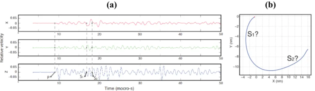
Figure 3.2: (a) Velocities of the particle motion on the surface of the sample B shown in Figure 3.1d at direction x, y and z against time. (b) Hodogram showing clear S-wave splitting of S1 and S2 registered by the LDI device on sample B. A time window between 17.42 to 18.50 micro-s is used to produce the hodogram.

LDI setup is shown in Figure 3.1a (Lebedev et al., 2011), The time-dependent displacement of a particular point on the sample surface in three independent directions was measured and transformed to cartesian coordinates to achieve three-component (3C) data (Figure 3.2a).

The anisotropy of these two samples are clear, as Malehmir et al. (2011) showed. In the exam-ple shown in Figure 3.2, we clearly observe shear-wave splitting (S1 and S2), which is already an indication of anisotropy in the sample.

3.2

Inversion

Different experiments and theoretical investigations have been carried out on different materi-als attempting to estimate full elastic stiffness tensor. Vestrum (1994) used a generalized linear inversion method to calculate all the elements of the tensor. He assumed no symmetry and ob-tained all components of the tensor. He carried out his experiment for both group and phase velocities. But here, I assumed that phase velocities were measured, which is a reasonable guess according to the size of the sample and the source. Moreover, the formulation here were ex-tracted from Vestrum (1994).

Here, a modified version of Vestrum's original code is deployed. The code is relatively straight-forward and uses no assumption about the symmetry of the sample in order to recover all the 21 components of the elastic stiffness tensor. Using LDI device, we measured phase velocities (P, S1 and S2) on the sample surface (Figure 3.1). At least a few shear-wave points are needed for the inversion to stabilize the result.

The code starts with an elastic stiffness tensor as an initial guess, after linearizing the prob-lem around the initial guess; using a linear least-square inversion method, it finds out a new guess in which the average squared phase velocity error (calculated with the measured ones) is minimized. This is done in an iterative manner until it reaches to a stage that the average squared error stops decreasing. In the inversion part, Christoffel's equation (Equation 2.8) is used for the forward modelling and in order to control validity of the results, velocities with more than 1 percent error to the measured ones will be eliminated in each step; velocities are computed from the forward modeling.

The ultimate goal of the inversion code is to minimize the difference between the observed phase velocities and the calculated ones via:

δvi = αji∆i, (3.1)

where Cj is the jth element of stiffness matrix (j varies between 1 and 21) and using the matrix

notation: δvi = viobs− v calc i , αji = ∂vj ∂Cj ∆i = ∆Cj,

The difference between the observed and calculated phase velocities (δvi) can be calculated

with:

− →

∆ = [eαTeα + λI]−1eαT−→δv. (3.2)

where λ is a small scalar quantity, which is added to diagonal of the matrix to be inverted in order to damp the solution and stabilize the inversion process.

3.3

Results

A summary of the measured values are shown in Table 3.1.

Table 3.1: Velocities in m/s, densities in kg/m3_{and thicknesses in mm.}

ID VP (0) VP(min) VP(max) VS(min) VS(max) Density Thickness

A 6450 6000 6450 3600 4000 2953 76.95

sample A: C =             21.9 34.3 50.4 −0.37 4.27 −0.08 34.3 53.9 79.2 −0.58 6.72 −0.12 50.4 79.2 117 −0.85 9.89 −0.18 −0.37 −0.58 −0.85 0.02 −0.07 0.0005 4.27 6.72 9.89 −0.07 0.84 −0.01 −0.08 −0.12 −0.18 0.0005 −0.01 0.02             , (3.3)

If 3.3 is rewritten by neglecting the small negative values in the matrix, 3.4 will be reached which looks like a Monoclinic symmetry. It will be discussed briefly in next section.

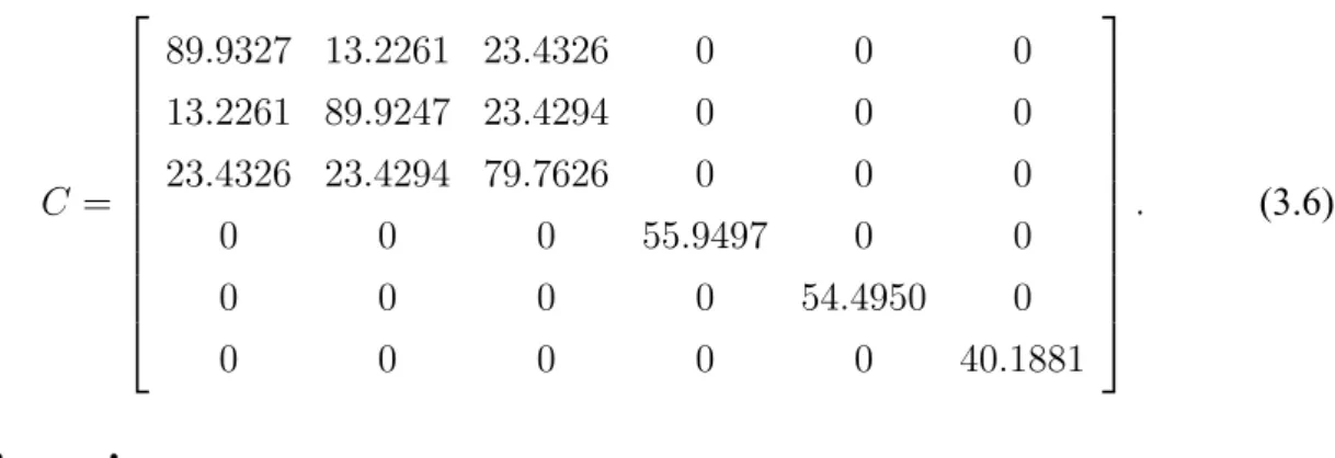
C =             21.9 34.3 50.4 0 4.27 0 34.3 53.9 79.2 0 6.72 0 50.4 79.2 117 0 9.89 0 0 0 0 0.02 0 0.0005 4.27 6.72 9.89 0 0.84 0 0 0 0 0.0005 0 0.02             . (3.4) sample B: C =             89.9327 13.2261 23.4326 −0.0008 0.0076 0.0000 13.2261 89.9247 23.4294 −0.0033 0.0018 0.0000 23.4326 23.4294 79.7626 0.0041 −0.0095 0.0000 −0.0008 −0.0033 0.0041 55.9497 0.0000 0.0028 0.0076 0.0018 −0.0095 0.0000 54.4950 −0.0011 0.0000 0.0000 0.0000 0.0028 −0.0011 40.1881             , (3.5)

Assuming the small values to be due to noise error and simply neglecting and replacing them with zero, an Orthorhombic symmetry is being reached:

C =             89.9327 13.2261 23.4326 0 0 0 13.2261 89.9247 23.4294 0 0 0 23.4326 23.4294 79.7626 0 0 0 0 0 0 55.9497 0 0 0 0 0 0 54.4950 0 0 0 0 0 0 40.1881             . (3.6)

3.4

Discussion

For sample A, only 12 measurements of P-waves and 3 measurements of both S-waves were used, which are not enough to obtain a unique solution. Some elements of sample A seem prob-lematic like the elements below one in the matrix 3.4. Moreover, as it is shown in Figure 3.1c, sample A is fairly folded and strongly deformed. So, the inversion might have failed in this case due to the complicated form of anisotropy and lack of sufficient data.

For sample B, 18 measurements of P-waves and 3 measurements of both S-waves were used, which are enough to obtain a unique solution. The results for sample B, more or less, are con-sistent with the previous studies (Malehmir et al., 2013). As it is shown in Table 3.2, there is a small difference between C44 and C55that made this result Orthorhombic but it is sufficiently

near to the previous study result. Hence, I decided not to rely on sample A for the next section. This explains why results from sample B are only shown in the next section. Please note that the nearest class of anisotropy for sample B is Orthorhombic.

The new results and those from previous study (Malehmir et al., 2013) for sample B are shown in Table 3.2. Please note the classes of symmetry in both case. This thesis shows slightly dif-ferent results from the previous study but they are reasonably close to each other.

Table 3.2: Comparison of the results with the previous study (Malehmir et al., 2013) for the sample B, all CIJ components are in GPa.

C11 C22 C33 C44 C55 C66 Symmetry

Previous study 104.8 104.8 91.9 33.3 33.3 38.2 TI (folded) This thesis 89.9 89.9 79.8 55.9 54.5 40.2 Orthorhombic

And the phase velocities for sample B in m/s is: • If Isotropic, according to the equation 2.19:

VP=5834 and VS=4602.

• If TI, according to the equations 2.20 to 2.22: VP=5497, VSV=4871 and VSH=4144.

• If TI, according to the Thomsen's approximation for weak anisotropy via the equations 2.30 to 2.32:

VP≈5809, VSV≈4507 and VSH≈4167.

• If TI, according to the Berryman's approximation for stronger anisotropy via the equations 2.33 and 2.34:

VP≈5791 and VSV≈4528.

• If Orthorhombic, according to equations 2.23 and 2.24: VP=6393 and VSV=3541.

Looking at the values of maximum P- and S-wave velocities in the Table 3.1 and comparing them with the above results show that the assumption of Orthorhombic as a class of symmetry for sample B is reasonable (note that the result of different TI approximations for VS is fairly

high but the Orthorhombic approximation seems convincing in both velocities).Thus, the LDI inversion results for sample B suggest Orthorhombic anisotropy and anisotropy parameters ob-tained here will be used in the next chapter for reprocessing the actual seismic data using an anisotropic processing approach.

4

Real Seismic Data

4.1

Background

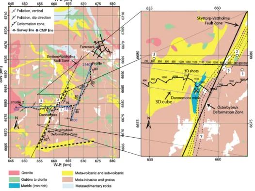
As it was mentioned earlier including anisotropy has an important role in exploration seismol-ogy and physical property studies are an essential prerequisites to design any seismic survey for crustal seismic imaging (Helbig and Thomsen, 2005; Tsvankin et al., 2010; Malehmir et al., 2013). Figure 4.1 shows the geological map of the study area and the location of the seismic profiles acquired in the previous study. The acquisition parameters and processing steps from previous study by Malehmir et al. (2011) without considering anisotropy are shown in Table 4.1. Malehmir et al. (2011) implied that the velocity anisotropy plays an important part in the

Figure 4.1:Geological map of the study area (zoomed in the right figure). Crooked-black line is the location of the seismic profile 2, the focus of this study; dashed lines show the inferred location of the deformation zone. The samples from location 1 and 2 are samples A and B respectively (modified from Malehmir et al., 2011).

reflections from the deformation zones in the study area. So, we want to introduce anisotropy to the same processing steps of the real seismic data acquired over the major deformation zone (the Österbybruk Deformation Zone) to examine if by introducing anisotropy, the seismic im-age of the ÖDZ improves. This, then, can somewhat support if anisotropy is playing a role in

Table 4.1: Acquisition parameters and processing steps of Dannemora data by Malehmir et al. (2011) without considering anisotropy.

Acquisition Parameters Processing Steps Parameters Unit Step Parameters

Survey Parameters 1 Read 21 s uncorrelated seismic data Recording system SERCEL 408UL 2 Data correlation and reduction to 3 s Profile 1 and 2 3 Building geometry data Spread geometry Asymmetric split spread 4 Trace editing

(100 stations arm) 5 Pick first breaks: full offset range automatic No. of live channels 360 neural network algorithm but manually Maximum offset 7200 m inspected and corrected

Survey length profile 2, around 21 km 6 Refraction static and elevation static Source VIBSIST corrections: datum 40 m, replacement Normal CMP fold 75 velocity 5800 m/s, v01000m/s

7 Geometric-spreading compensation: v2_t

Spread Parameters 8 Band-pass filtering: 20-35-150-170 Hz Receiver spacing 20 m (reduced to 10 m 9 Surface-consistent deconvolution: filter

around Dannemora) 140 ms, gap 15 ms, white noise 0.1% Source interval 40 m (reduced to 10 m 10 Band-pass filtering: 20-30-140-160 Hz

around Dannemora) 11 Top mute: 30 ms after first breaks Recording length 21 s (3 s after decoding) 12 Direct shear wave attenuation (near-offset) Sampling rate 1 ms 13 Air blast attenuation

14 Trace balance using data window Receiver and Source Parameters 15 Velocity analysis (iterative) Geophone frequency 28 Hz 16 Residual static corrections (iterative) Geophone per set Single 17 Normal moveout corrections (NMO): Sweeps 3-5 60% stretch mute

Shots 1350 18 Stack

To simplify the result and prior to highlighting the effect of anisotropy from the lab data to the real seismic data, I take your attention in following:

• The importance of different frequencies used in the lab and in the seismic data should not be underestimated and its contribution (and to what extent) should further be investigated using real field 3C data;

• One or a few samples (five samples in this study were used) may not be representative of the whole deformation zone thus our results provide first order information about the anisotropy until more data and experiments are conducted;

• In this study, the nearest form of anisotropy is assumed, orthorhombic here, to the in-version result for the data processing to be able to use the Tsvankin's dimensionless anisotropic parameters and the non-hyperbolic moveout equation (Equation 2.39).

4.2

From The Laboratory to the Real Data

The stiffness tensor of an orthorhombic media in two-index Voigt notation is:

C =             C11 C12 C13 0 0 0 C12 C22 C23 0 0 0 C13 C23 C33 0 0 0 0 0 0 C44 0 0 0 0 0 0 C55 0 0 0 0 0 0 C66             . (4.1)

So, stiffness tensor in the mentioned notation for sample B would be:

C =             89.9327 13.2261 23.4326 0 0 0 13.2261 89.9247 23.4294 0 0 0 23.4326 23.4294 79.7626 0 0 0 0 0 0 55.9497 0 0 0 0 0 0 54.4950 0 0 0 0 0 0 40.1881             . (4.2)

4.3

Results

Knowing the limitation mentioned in section 4.1, we can use the Tsvankin's extension of the Thomsen's parameters for orthorhombic media, which was briefly described in section 2.7, to in-troduce anisotropy to the processing steps of the Dannemora data via the non-hyperbolic move-out equation (Equation 2.39).

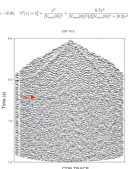
The event marked by arrow in CDP 1621 over the deformation zone, shown in Figure 4.2, is used to compute three dimensionless coefficients (equations 2.35 to 2.37) in order to calcu-late η (Equation 2.38) to use in the non-hyperbolic moveout equation (Equation 2.39). These are the results obtained:

thus: η =−0.35, t2(x) = t2₀+ x 2 [Vnmo(0)]2 + 0.7x 4 [Vnmo(0)]2{t20[Vnmo(0)]2+ [0.3]x2} . 0.0 0.5 1.0 1.5

T

im

e

(s)

CDP TRACE

Figure 4.2: An example CDP gather (CDP 1612) after applying NMO correction; the event marked by the red arrow is used to extract parameters for the non-hyperbolic moveout equation at this location and time.

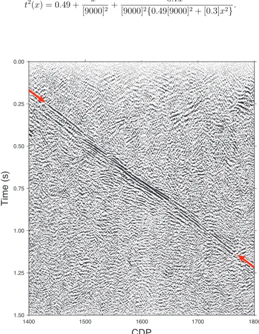
For the event marked by the red arrow in Figure 4.2 we will have: t0 = 700 ms and VN M O(0) = 9000 m s =⇒ t2(x) = 0.49 + x 2 [9000]2 + 0.7x4 [9000]2{0.49[9000]2_{+ [0.3]x}2}. (4.3) 0.00 0.25 0.50 0.75 1.00 1.25 1.50

T

im

e

(s)

CDP

Figure 4.3: Unmigrated stacked section of the deformation zone before introducing anisotropy parameters into the processing steps (after Malehmir et al., 2011); Reflection package in between two arrows is interpreted to be from the deformation zone, CDP spacing is 10 m.

after (Figure 4.4) introducing anisotropy parameters into the processing steps. 0.00 0.25 0.50 0.75 1.00 1.25 1.50

T

im

e

(s)

CDP

Figure 4.4:Unmigrated stacked section of the deformation zone after introducing anisotropy parameters into the processing steps (this study); Reflection package in between two arrows is interpreted to be from the deformation zone, CDP spacing is 10 m.

To highlight the effect of introducing anisotropy to the processing steps, we shall take a closer look at the unmigrated stacked section crossing the deformation zone before (Figure 4.5a) and after (Figure 4.5b) introducing anisotropy parameters into the processing steps. Please note partial improvement in the circled areas.

(a) 0.0 0.5 1.0 1.5 T im e (s) 1500 CDP 1600 1700 (b) 0.0 0.5 1.0 1.5 T im e (s) 1500 CDP 1600 1700

Figure 4.5: A closer look to the unmigrated stacked section crossing the deformation zone (a) before and (b) after introducing anisotropy parameters into the processing steps. Please note partial improvement in the circled area

Finally, in Figure 4.6 you can see portions of the unmigrated stacked section crossing the de-formation zone before (Figure 4.6a and 4.6c) and after (Figure 4.6b and 4.6d) introducing the anisotropy parameters into the processing steps (this study). Again please note partial improve-ments marked on the section by the red arrows.

4.4

Discussion

As it is briefly shown in Figures 4.3 - 4.6, introducing anisotropy to the processing steps at least partially improves the unmigrated stacked section crossing the deformation zone. Moreover, If we see the velocity versus azimuth plot, we might see further support for the presence of

(a) (b)

(c) (d)

Figure 4.6: Portions of the unmigrated stacked section crossing the deformation zone (a) and (c) before, (b) and (d) after introducing the anisotropy parameters into the processing steps (this study). Note partial improvements marked on the sections by the red arrows. CDP spacing is 10 m.

fitted curve over the whole data using an 8-order sinusoidal line with the following details:

4% 8% 12% WEST EAST SOUTH NORTH 0 − 500 500 − 1000 1000 − 1500 1500 − 2000 2000 − 2500 2500 − 3000 >=3000

0 60 120 180 240 300 360 0 1000 2000 3000 4000 5000 6000 7000 8000 9000 10000 Azimuth (degree) Ve lo ci ty (m/ s )

Figure 4.8: P-wave direct arrival velocity measured over the deformation zone with respect to the azimuth. Please note that each dot represent one P-wave arrival velocity and the red line is a fitted curve using MATLAB curve fitting application. The graph may suggest an NE-SW anisotropy direction that correlate well with the strike of the ÖDZ observed in the geological map.

General model Sin8:

f (x) =

a1sin(b1x + c1) + a2sin(b2x + c2) + a3sin(b3x + c3) + a4sin(b4x + c4)+

a5sin(b5x + c5) + a6sin(b6x + c6) + a7sin(b7x + c7) + a8sin(b8x + c8),

where x is normalized by mean value of 167.8 and standard deviation of 93.4, with these coef-ficients (with 95% confidence bounds):

a1 = 1.463e + 04, b1 = 0.6891, c1 = 1.695, a2 = 9768, b2 = 0.911, c2 =−1.4, a3 = 485.1, b3 = 3.763, c3 =−1.114, a4 = 72.97, b4 = 6.335, c4 =−5.14, a5 = 224.3, b5 = 8.877, c5 =−0.03853, a6 = 28.19, b6 = 26.85, c6 =−2.696,

a7 = 186.6, b7 = 9.746, c7 = 2.516, a8 = 161.3, b8 = 11.07, c8 =−0.102.

In general, the reflection seismic data show at least partial improvement; So, introducing anisotropy into the processing steps not only seems helpful and promising but also to some extent necessary and crucial for the processing results.

5

Conclusions

Phase velocity data, measured by LDI device, were successfully inverted to elastic stiffness ten-sor without assuming any kind of symmetry as a priori information. This maybe the first time that a general inversion code is deployed for the LDI measurements to obtain stiffness tensor. The inversion was stable and fast likely due to the rich and often consistent input data (at least for the sample B).

Inversion results suggest an Orthorhombic media (for sample B), more or less consistent with the previous studies suggesting fairly similar anisotropy system for the major deformation zone. This was further supported by other approximation for quasi-P and quasi-s wave velocities for anisotropic media.

New processing results show partial reflection improvement when the Orthorhombic anisotropy parameters were introduced into the processing steps. This fact suggests that anisotropy has a crucial role in processing results and should be included in the whole procedure.

Future studies should aim at:

• Collecting more rock samples in order to reach to better results and to be able to improve whole reflection package, generated by the deformation zone.

• Using synthetic data to study both parts (inversion and real data) more specifically in or-der to better unor-derstand the probable causes of failure of this method.

• Better understanding the relationship between the seismic frequency and lab measure-ments for rock samples from crystalline rock environment often characterized by low-porosity and high-degree of solidification.

6

References

Alkalifah, T. and Tsvankin, I. (1995). Velocity analysis for transversely isotropic media. Geo-physics, 60:1550--1566.

Allen, R. L., Lundström, I., Ripa, M., Simenov, A., and Christofferson, H. (1996). Facies analysis of a 1.9 ga, continental margin, back�arc, felsic caldera province with diverse zn�pb�ag�(cu�au) sulfide and fe oxide deposits, bergslagen region, sweden. Econ. Geol., 91:979--1008.

Antal, I., Bergman, S., Gierup, J., Persson, C., and Thunholm, B. (1998). Översiktsstudie av uppsala län--geologiska förutsättningar, rep. r�98� 32, 49 pp., svensk kärnbränslehantering ab. Stockholm, Sweden.

Arts, R. (1993). A study of general anisotropic elasticity in rocks by wave propagation: Theo-retical and experimental aspects. PhD thesis, Institut Français du Pétrole.

Arts, R., Rasolofosaon, N., and Zinszner, B. (1991). Complete inversion of the anisotropic elastic tensor in rocks: Experiment versus theory: 1991 technical program. 61st Annual International SEG Meeting, Expanded Abstracts, pages 1538--1540.

Bayón, A. and Rasolofosaon, P. N. J. (1996). Three-component recording of ultrasonic transient vibration by optical heterodyne interferometry. Journal of the Acoustical Society of America, 99:954--961.

Bergman, S., Isaksson, H., Johansson, R., Linden, A., Persson, C., and Stephens, M. (1996). Förstudie östhammar, jordarter, bergarter och deformationszoner, skb djupförvar, rep. pr d�96�016, 81 pp., svensk kärnbränslehantering ab. Stockholm, Sweden.

Berryman, J. (2008). Exact seismic velocities for transversely isotropic media and extended thomsen formulas for stronger anisotropies. Geophysics, 73:D1--D10.

Crampin, S. (1981). A review of wave motion in anisotropic and cracked elastic media. Wave Motion, 3:343--391.

Crampin, S. (1985). Evaluation of anisotropy by shear-wave splitting. Geophysics, 50:142--152.

Dahlin, P. and Sjöström, H. (2010). Structure and stratigraphy of the dannemora inlier, eastern bergslagen region: Primary volcanic textures, geochemistry and deformation, 91 pp., sveriges

Fukushima, Y., Nishizawa, O., Sato, H., and Ohtake, M. (2003). Laboratory study on scatter-ing characteristics of shear waves in rock samples. Bulletin of the Seismological Society of America, 93:253--263.

Helbig, K. and Thomsen, L. (2005). 75--plus years of anisotropy in exploration and reservoir seismics:ahistorical review of concepts and methods. Geophysics, 70(6):9ND--23ND.

Jech, J. (1991). Computation of elastic parameters of anisotropic medium from traveltimes of quasicompressional waves. Physics of the Earth and Planetary Interiors, 66:153--159.

Juhlin, C. and Stephens, M. B. (2006). Gently dipping fracture zones in paleoproterozoic meta-granite, sweden: Evidence from reflection seismic and cored borehole data, and implications for the disposal of nuclear waste. Journal of Geophysical Research, page B09302.

Lebedev, M., Bona, A., Pevzner, R., and Gurevich, B. (2011). Elastic anisotropy estimation from laboratory measurements of velocity and polarization of quasi-p-waves using laser in-terferometry. Geophysics, 76:WA83--WA89.

Lynn, H. B. and Thomsen, L. (1986). Shear wave exploration along the principal axis. 56th Annual International Meeting, SEG, Expanded Abstracts, pages 474--476.

Mah, M. and Schmitt, D. R. (2003). Determination of the complete elastic stiffnesses from ultrasonic phase velocity measurements. Journal of Geophysical Research, 108(B1):2016.

Malehmir, A., Andersson, M., Lebedev, M., Urosevic, M., and Mikhaltsevitch, V. (2013). Ex-perimental estimation of velocities and anisotropy of a series of swedish crystalline rocks and ores. Geophysical Prospecting, 61:153--167.

Malehmir, A., Dahlin, P., Lundberg, E., Juhlin, C., Sjöström, H., and Högdahl, K. (2011). Reflection seismic investigations in the dannemora area, central sweden: Insights into the geometry of polyphase deformation zones and magnetite�skarn deposits. Journal of Geo-physical Research, 116:B11307.

Martin, D., Pouet, B., and Rasolofosaon, P. N. J. (1994). Laser ultrasonics applied to seismic physical modeling, in d. a. ebrom, and j. a. mcdonald, eds., seismic physical modeling. SEG Geophysics Reprint Series 15, pages 499--511.

Mavko, G., Mukerji, T., and Dvorkin, J. (2009). The Rock Physics Handbook: Tools for Seismic Analysis of Porous Media. Cambridge University Press, second edition.

Nishizawa, O., Satoh, T., Lei, X., and Kuwahara, Y. (1997). Laboratory studies of seismic wave propagation in inhomogeneous media using a laser doppler vibrometer. Bulletin of the Seismological Society of America, 87:809--823.

Pouet, B. and Rasolofosaon, P. N. J. (1990). Seismic physical modeling using laser ultrasonics. 60th Annual International Meeting, SEG, Expanded Abstracts, pages 841--844.

Rasolofosaon, P. N. J., Martin, D., Gascon, F., Bayón, A., and Varade, A. (1994). Physical modeling of 3d seismic wave propagation, in k. helbig, ed., modeling the earth for oil ex-ploration: Final report of the cec's geoscience i program, 1990-93. Pergamon Press, pages 637--686.

Stålhös, G. (1991). Beskrivning till berggrundskartorna östhammar nv, no, sv, so: med sam-manfattande översikt av basiska gångar, metamorfos och tektonik i östra mellansverige, ser. af 161, 166, 169, 172, 249 pp., sveriges geologiska undersökning. Uppsala, Sweden.

Stephens, M. B., Ripa, M., Lundström, I., Persson, L., Bergman, T., Ahl, M., Wahlgren, C. H., Persson, P., and Wickström, L. (2009). Synthesis of the bedrock geology in the region, fennoscandian shield, south�central sweden. Rep. Ba 58, 259 pp., Geol. Surv. of Swed., Uppsala, Sweden.

Thomsen, L. (1986). Weak elastic anisotropy. Geophysics, 51:1954--1966.

Tsvankin, I. (1997). Anisotropic parameters and p-wave velocity for orthorhombic media. Geo-physics, 62(4):1292--1309.

Tsvankin, I., Gaiser, J., Grechka, V., van der Baan, M., and Thomsen, L. (2010). Seis-mic anisotropy in exploration and reservoir characterization: An overview. Geophysics, 75(5):75A15--75A29.

Vestrum, R. W. (1994). Group and phase-velocity inversions for the general anisotropic stiffness tensor. Master's thesis, University of Calgary.

Willis, H., Rethford, G., and Bielanski, E. (1986). Azimuthal anisotropy: The occurence and effect on shear wave data quality. 56th Annual International Meeting, SEG, Expanded Ab-stracts, pages 479--481.

Tidigare utgivna publikationer i serien ISSN 1650-6553

Nr 1 Geomorphological mapping and hazard assessment of alpine areas in

Vorarlberg, Austria, Marcus Gustavsson

Nr 2 Verification of the Turbulence Index used at SMHI, Stefan Bergman

Nr 3 Forecasting the next day’s maximum and minimum temperature in Vancouver,

Canada by using artificial neural network models, Magnus Nilsson

Nr 4 The tectonic history of the Skyttorp-Vattholma fault zone, south-central Sweden,

Anna Victoria Engström

Nr 5 Investigation on Surface energy fluxes and their relationship to synoptic weather

patterns on Storglaciären, northern Sweden, Yvonne Kramer

Nr 255 Kai XueThe Effects of Basal Friction and Basement Configuration on

Deformation of Fold-and-Thrust Belts: Insights from Analogue Modeling,      

Kai Xue, Mars 2013

Nr 256 Water quality in the Koga Irrigation Project, Ethiopia: A snapshot of general

quality parameters.Vattenkvalitet i konstbevattningsprojektet i Koga, Etiopien: En överblick av allmänna kvalitetsparametrar. Simon Eriksson, Mars 2013

Nr 257 3D Processing of Seismic Data from the Ketzin CO2 Storage Site, Germany.

Jawwad Ashraf Qureshi, April 2013

Nr 258 Investigations of Manual and Satellite Observations of Snow in Järämä (North

Sweden) Daniel Pinto, May 2013

Nr 259 Jämförande studie av två parameterskattningsmetoder i ett grundvattenmagasin.

Comparative study of two parameter estimation methods in a groundwater aquifer.

Stefan Eriksson, May 2013

Nr 260 Case Study of Uncertainties Connected to Long-term Correction of Wind

Observations. Elisabeth Saarnak, May 2013

Nr 261Variability and change in Koga reservoir volume, Blue Nile, Ethiopia . Variabilitet

och förändring i Koga dammens vattenvolym, Blå Nilen, Etiopien. Benjamin Reynolds, May 2013

Nr 262 Meteorological Investigation of Preconditions for Extreme-Scale Wind Turbines

in Scandinavia. Christoffer Hallgren, May 2013

Nr 263 Application of the Reflection Seismic Method in Monitoring CO2 Injection in a

Deep Saline Aquifer in the Baltic Sea. Saba Joodaki, May 2013