Anisotropic geometrical-spreading correction and its application in azimuthal AVO analysis

IN AZIMUTHAL AVO ANALYSIS

by

Philosophy (Geophysics). Golden, Colorado

Date /y''^ ^

■

O,

^

Date ^^0^-

ILOO^

Velocity vaxiations with angle in anisotropic media influence not only reflection coefficients but also geometrical spreading. Anisotropy-induced distortions in geo metrical spreading can be comparable to those in reflection coefiicients. Since AVO (amplitude-variation-with-oflFset) analysis operates with reflection coefficients, an im

portant element of AVO processing, particularly for azimuthaJ AVO, is to correct amplitude responses for anisotropic geometrical spreading.

Using paraxial ray theory, I obtain a concise expression for geometrical spreading

as a function of reflection traveltimes recorded over laterally homogeneous, arbitrar

ily anisotropic media. By extending the Alkhalifah-Tsvankin (1995) nonhyperbolic moveout equation to orthorhombic media, I further express azimuthally-vaxying geo metrical spreading in terms of normal-moveout velocities and anellipticity parameters. Weak-anisotropy approximation reveals that the azimuthal variation of geometrical spreading is primarily controlled by the difference between the anellipticity parame

ters in the two vertical symmetry planes of orthorhombic media.

Using the analytic results, I develop a moveout-based anisotropic spreading correction (MASC) that computes geometrical spreading from estimated normal-moveout velocities and anellipticity parameters. The implementation of MASC in volves almost no extra cost; the spreading correction can be incorporated easily into the processing sequence that estimates azimuthal moveout and AVO attributes. MASC proves to be insensitive to the trade-offs between moveout velocities and anel lipticity parameters as long as they approximate the traveltime surface with adequate accuracy. Sensitivity studies show that the robustness of MASC is lower than that

The underlying assumption of the MASC methodology is that the medium is laterally homogeneous. I perform numerical modeling to show that MASC remains sufficiently accurate for media with mild reflector dip and moderate lateral velocity variation. Because of the high sensitivity of shear waves to the presence of anisotropy, it is imperative to correct for geometrical spreading in AVO analysis of converted PS-waves. I, therefore, extend the MASC algorithm to PS-waves. The formalism developed for P-waves can be used to correct for the geometrical spreading for PS-waves, albeit with slightly lower accuracy.

To evaluate the accuracy of MASC and its significance for azimuthal AVO anal ysis, I apply anisotropic spreading correction to wide-azimuth full-wavefield synthetic data and field data. Synthetic studies on models with strong azimuthal anisotropy verify the accuracy of MASC. In addition, I show that application of MASC is criti cally important for accirrate quantitative AVO inversion. For qualitative AVO anal ysis, application of MASC becomes essential when the magnitude of the azimuthal variation of geometrical spreading reaches about one-third of that of the correspond ing reflection coefficient. Also, I demonstrate that the influence of transmission loss on azimuthal AVO analysis of P-waves is negligible. Application of MASC to

wide-azimuth data from the Rulison field, Colorado, confirms that MASC is essential for reliable estimation of azimuthal AVO attributes. In addition, the field study proves the stability of azimuthal AVO attributes and helps to improve understanding of the fracture distribution in the reservoir.

ABSTRACT iii

LIST OF FIGURES viii

LIST OF TABLES xvii

ACKNOWLEDGMENTS xix

Chapter 1 INTRODUCTION 1

Chapter 2 GEOMETRICAL SPREADING OF P-WAVES IN HORIZONTALLY

LAYERED, AZIMUTHALLY ANISOTROPIC MEDIA 9

2.1 Summary 9

2.2 Introduction 10

2.3 Relative geometrical spreading as a function of reflection traveltime . 12 2.3.1 Nonhyperbolic moveout equation for an orthorhombic layer . . 16

2.3.2 Geometrical spreading as a function of moveout coefficients . . 21 2.3.3 Analysis of the weak-anisotropy approximation 22

2.3.4 Numerical example 25

2.4 Comparison with dynamic ray tracing 29

2.5 Discussion and conclusions 32

2.6 References 37

Chapter 3 ANISOTROPIC GEOMETRICAL-SPREADING CORRECTION FOR

WIDE-AZIMUTH P-WAVE REFLECTIONS 40

3.1 Summary 40

3.2 Introduction 41

3.3 Moveout equations for orthorhombic media 43

3.3.1 Layered models with uniform symmetry-plane orientation . . . 45 3.3.2 Models with misaligned symmetry planes 48 3.4 Azimuth-dependent geometrical-spreading correction 52

3.4.1 Synthetic example 54

Chapter 4 ESTIMATION OF

REFLECTION COEFFICIENTS ON

FULL-WAVEFORM

SYNTHETIC DATA 71

4.1 Introduction 71

4.2 Synthetic modeUng 74

4.3 Estimation of the reflection coefficient from the AVO response . . . . 76

4.3.1 Model 1 77

4.3.2 Model 2 81

4.3.3 Model 3 84

4.4 Influence of the transmission loss 87

4.5 Discussion 87

Chapter 5 CASE

STUDIES

OF

AZIMUTHAL

AVO

ANALYSIS WITH

ANISOTROPIC

SPREADING CORRECTION 92

5.1 Introduction 92

5.2 Geologic background 94

5.3 Data acquisition and processing 94

5.4 Results of azimuthal seismic analysis 103

5.4.1 Mesaverde top 103

5.4.2 Top of the reservoir (UMV Shale) 103

5.4.3 Bottom of the reservoir (Cameo Coal) 107 5.5 Comparison with the fault system and EMI log 110

5.5.1 Fault system 110

5.5.2 EMI and production logs Ill

5.6 Discussion 112

5.6.1 Acquisition footprint 112

5.6.2 Error analysis 113

5.6.3 Correlation between the NMO and AVO ellipses 114

5.6.4 Group angle versus phase angle 114

5.7 Conclusions 116

5.8 References 116

Chapter 6 ANISOTROPIC GEOMETRICAL-SPREADING CORRECTION IN THE PRESENCE OF LATERAL HETEROGENEITY 119

6.1 Introduction 119

6.2 Numerical tests 120

6.3 Conclusions 126

6.4 References 126

Chapter 7 MASC FOR CONVERTED PS-WAVES 127

7.1 Introduction 127

7.2 Moveout-based expression for geometrical spreading of PS-waves . . . 128 7.3 Algorithm for moveout-based anisotropic spreading correction . . . . 132 7.4 Application to AVO analysis of synthetic data 141

7.5 Conclusions 143

7.6 References 144

Chapters CONCLUSIONS 146

APPENDIX A RELATIVE GEOMETRICAL SPREADING AS A FUNCTION

OF REFLECTION TRAVELTIME 151

APPENDIX B TRAVELTIME DERIVATIVES FROM THE NONHYPERBOLIC

MOVEOUT EQUATION 155

APPENDIX C TRAVELTIME DERIVATIVES FOR THE

GEOMETRICAL-SPREADING CORRECTION 157

1.1 P-wave propagation from a point source (triangle) in a vertical plane

of a homogeneous VTI medium with e = 0.15 and 5 = —0.1. The rays

(in black) are computed with a constant increment in phase angle; the

wavefront is shown in white. Notice that the density of rays strongly

varies with angle (after Tsvankin, 2005) 2

1.2 SV-wave propagation from a point source (triangle) in a vertical plane of a homogeneous VTI medium with e = 0.15 and 5 = —0.1 (a = 0.42). The rays (in black) are computed with a constant increment in phase

angle; the wavefront is shown in white. Notice the concentration of

rays near the velocity maximum at an angle of 45° (after Tsvankin,

2005) 3

2.1 Reflected ray in a homogeneous horizontal orthorhombic layer with a horizontal symmetry plane. The ray lies in the incidence plane, al

though the corresponding phase-velocity vector may point out of plane. 15

2.2 Sketch of body-wave phase-velocity surfaces in orthorhombic media

(after Grechka et al., 1999). Tsvankin's (1997) parameters axe defined in the mutually orthogonal symmetry planes which coincide with the coordinate planes. A marks a point (conical) singularity where the

phase velocities of the two S-waves are equal to each other 17

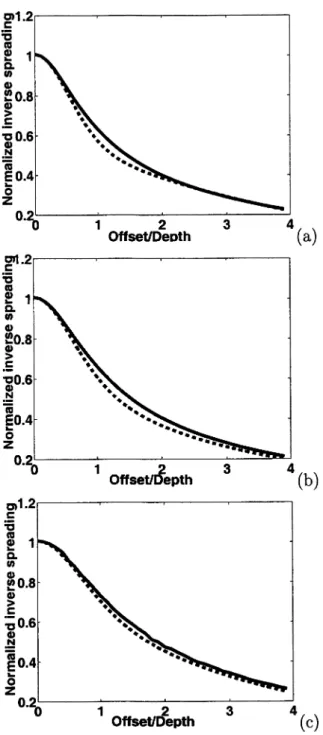
2.3 Normalized inverse spreading as a function of the oflfset-to-depth ratio in the symmetry planes [xi,a:3] (a) and [x2, X3] (b) of a horizontal orthorhombic layer. The solid line is computed using equations (2.5) and (2.10), the dashed line is the weak-anisotropy approximation, and the dotted line is L~^ in the reference VTI model. The model param

eters axe VpQ =

2.437 km/s,

=

0.329,

=

0.258, (5^^^ =

0.083,

(5^^) = —0.078, and = —0.106. The corresponding P-wave moveout

parameters axe Vnmo =

2.632 km/s, Vnmo =

2.239 km/s, 77^^^ =

0.211,

7y(2) = 0.398, and — 0.193. The inverse spreading L~^ is normal

ized by its value in the corresponding isotropic layer with the velocity

Vpo = 2.437 km/s 27

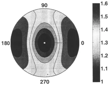
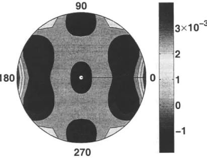
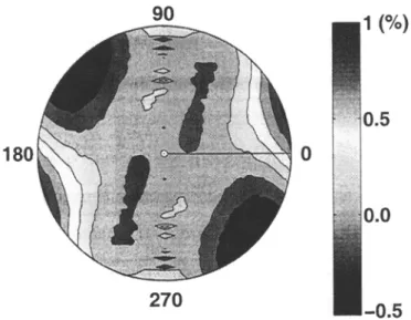
respect to the xi-axis. The solid line is computed using equations (2.5) and (2.10), the dashed line is the weak-anisotropy approximation. . . 30 2.5 Map of the normalized inverse spreading L~^ as a function of offset

and azimuth. Plot (a) is computed for the model from Figure 2.3; in plot (b), the sign of the parameter was changed from negative to

positive (i.e., 5^"^^ — 0.078). The oflFset-to-depth ratio varies from zero

to four 31

2.6 Comparison of the inverse relative spreading computed by our method (dashed line) and code ANRAY (solid) for the model from Figure 2.3. The source-receiver line is oriented (a) along the xi-axis; (b) at 45° with the xi-axis; and (c) along the a:2-axis 33 2.7 Comparison of the inverse relative spreading computed by our method

(dashed line) and code ANRAY (solid) for the layered orthorhombic model from Table 1 (we used the reflection from the bottom of the third layer). The source-receiver line is oriented (a) along the xi-axis; (b) at 45° with the ari-axis; and (c) along the X2-axis 34 3.1 Accuracy of equation 3.4 in describing full-azimuth, long-offset P-wave

moveout in a homogeneous orthorhombic layer. The moveout param

eters are found by fitting equation 3.4 to traveltimes computed by anisotropic ray tracing. The map shows the difference between the best-fit and ray-traced traveltimes normalized by the zero-offset time

(0.82 s). The radius corresponds to the source-receiver offset (the max

imum offset-to-depth ratio is three), the numbers around the perime ter indicate the azimuth with respect to the [xi, 0:3] symmetry plane. The P-wave velocity parameters of the model are Vpo = 2.437 km/s, = 0.329, = 0.258, = 0.083, = -0.078, and =

(1)

—0.106. The corresponding moveout parameters are Vnmo = 2.632

km/s, Kml

=

2.239 km/s,

=

0.211, 77(2) =

0.398, and

=

0.194. 46

dashed line is the ray-traced traveltime for the reflection from the bot tom of layer 3, the solid line is the corresponding traveltime com puted from equation 3.4 with the following estimated (best-fit)

move-out parameters: (f) =

90°, vimo =

2.307 km/s, Vnmo — 2.675 km/s,

= 0.305, = 0.222, and = -0.006 49

3.3 Map of the traveltime residuals (normalized by the zero-offset time To = 1.334 s) plotted as a function of offset and azimuth for the

two-layer model with misaligned symmetry planes from Table 2

(model 2).

The residuals are computed for the reflection from the bottom of the model as the differences between the best-fit traveUmes from equa tion 3.4 and ray tracing. The maximum offset is 4 km; the correspond ing offset-to-depth ratio is two. The estimated moveout parameters are </> = 78°, = 2.60 km/s, = 3.00 km/s, = 0.567,

77(2) =

0.330, and 77(2) =

0.104

50

3.4 Comparison of the effective parameter 77(0;) computed from the VTI averaging equation 3.6 (solid curve) and estimated by the moveout-inversion algorithm (dashed). The model is composed of two orthorhom-bic layers; for the top layer, 4> = 15°, Inmo = 2.236 km/s, Inmo =

2.850 km/s, 77^^) =

0.375, 77(2) =

0.000, and 77(2) =

-0.086; for the bot

tom layer, (j) =

0°)

=

3.421 km/s,

Kmo

=

2.683 km/s,

77^^^ =

0.000,

7^(2) =

0.375, and 77^^^ =

0.163. The maximum offset-to-depth ratio of

the data used in the inversion is two 52

3.5 Same as Figure 3, but the moveout parameters of equation 3.4 were estimated by the modified inversion algorithm that allows for an in dependent orientation of the 77(Q!)-curve [equation 3.7]. The best-fit

parameters are 0

=

81°, Vnmo =

2.586 km/s,

=

3.00 km/s,

77^^) =

0.594,77(2) =

0.339,

=

0.161, and (f>i =

89°

53

3.6 Map of the geometrical spreading for the reflection from the bottom of layer 3 in model 1 (Table 1). The factor L is normalized by its value in the reference isotropic homogeneous medium with the velocity equal to Kmo = (Vlimo + V'nmo)/2. The maximum offset-to-depth ratio is two. 56

3.8 A7iTTmt.ha.lly varying reflection coefficient from the bottom of layer 3 in model 1 (Table 1) computed for the phase incidence angle at the

reflector equal to 30° 58

3.9 Accuracy of our method for the reflection from the bottom of layer 3 in model 1; the azimuths from the [xi, 0:3] symmetry plane are a = 0°, 40°, and 90°. The geometrical-spreading factor L computed by our algorithm (solid lines) is compared with the output of dynamic

ray-tracing code ANRAY (dashed) 59

3.10 Percentage error of the geometrical spreading for model 1 (Figure 3.6)

caused by the traveltime error function 4sin(37rx/xniax) sin4Q; (in ms).

The maximum offset-to-depth ratio is two 61

3.11 Histogram of the error distribution in the geometrical spreading com

puted in the [xijXs] symmetry plane of model 1 (Figure 3.6). The

moveout parameters were contaminated by Gaussian noise with the

following standard deviations: 0.5% for To, 3%

for Vnmo and Vnmo, 30%

for and and 50% for The offset-to-depth ratio is equal to

one (a) and two (b). The standard deviation of the error in L

is 5%

in

plot (a) and 8% in plot (b) 63

3.12 Map of the geometrical spreading for the P-wave reflection from the Mississippian formation (the top of the reservoir) at Weyburn field computed for CMP 10829. The factor L is normalized by its value in the reference isotropic homogeneous medium with the velocity equal to

{Vnmo +

14mo)/2. The moveout parameters are taken from Vasconcelos

and Tsvankin (2004): (f) =

99°, Wmo =

2.371 km/s, Vnmo =

2.464 km/s,

= 0.255, = 0.186, and = -0.062. The reflector depth is

1.4 km (the maximum offset-to-depth ratio is 2.5). The North-South

direction is at (^ = 0°, and the East-West at 0 = 90° 64 3.13 Normalized geometrical spreading from Figme 3.12 in the east-west

and north-south directions 65

is specifled as a halfspace to eliminate the influence of the free surface. The arrows mark the target PP-wave reflected from the bottom of the orthorhombic layer. The ellipses highlight the areas of interference of the target PP event with the PS and SS reflections from the top of the

orthorhombic layer 75

4.2 Synthetic gather for model 6.3 (Table 3) computed in the symmetry

plane [0:2, X3] (azimuth 90°) 76

4.3 Comparison of the reconstructed (dashed lines) and exact (solid lines)

reflection coefficients for the PP-wave reflected from the bottom of the orthorhombic layer in model 7.1. The reflection coefficient is estimated using (a) MASC; and (b) the t^-gain. The offset-to-depth ratio that corresponds to the maximum horizontal slowness (0.3 s/km) is slightly

larger than two 80

4.4 Comparison of the geometrical spreading computed by MASC (dashed lines) and dynamic ray tracing (solid) for the PP reflection from the

bottom of the orthorhombic layer in model 7.1 81

4.5 Comparison of the reconstructed (dashed lines) and exact (solid) reflec

tion coefficients for model 7.2. The reflection coefficient is estimated

using (a) MASC;

and (b)

the t^-gain. The reconstructed reflection co

efficients for the 45°- and 90°-azimuths on plot (b) practically coincide with one another; for the 0°-azimuth, the reconstructed coefficient is almost invisible because it is close to the exact value. The

offset-to-depth ratio that corresponds to the maximum horizontal slowness (0.3

s/km) is close to two 82

4.6 Comparison of the reconstructed (dashed lines) and exact (solid) reflec

tion coefficients for model 6.3. The reflection coefficient is estimated

using (a) MASC; and (b) the t^-gain. The offset-to-depth ratio that corresponds to the maximum horizontal slowness (0.3 s/km) is close to

2.5 85

4.7 Transmission loss for the PP reflection from the bottom of the or

thorhombic layer in (a) model 7.1; (b) model 7.2; and (c) model 6.3. The loss is computed by subtracting from unity the product of the plane-wave transmission coefficients along the raypath 88

is bounded by the UMV Shale and the Cameo Coal. The Mesaverde Top is an unconformity that separates the Mesaverde group from the

overlying Wasatch formation 95

5.3 Seismic acquisition grid for the RCP nine-component 2003 survey. . 96 5.4 P-wave fold for the 55x55 ft binsize. The square in the center encom

passes the study area of this paper 97

5.5 Seismic section across the middle of the survey area. The refiectors analyzed in the paper are marked on the plot 98

5.6 (a) A 5x5 CMP supergather at the north-west corner of om: study area; (b) the same gather after application of azimuthally-varying normal-moveout correction. The maximum offset for the gather is 7700 feet. The maximum offset-to-depth-ratios for the Mesaverde Top, the top of the reservoir (UMV Shale), and the bottom of the reservoir (Cameo

Coal) are 1.9, 1.5, and 1.1, respectively. 100

5.7 Distribution of offsets and azimuths for CMP superbins in the four corners of the study area. Note that full azimuthaJ coverage is achieved

for offsets up to around 5000 feet 102

5.8 AVO and NMO ellipse information extracted for the reflection from the Mesaverde Top. The three columns correspond to the AVO ellipses

computed using MASC (left), the AVO ellipses after application of the conventional gain correction (center), and the effective NMO ellipses (right). The three rows show the eccentricity of the ellipses (top), the azimuths of the major principal axis of the ellipses (middle), and the rose diagram of the orientation of the major principal axis (bottom).

The eccentricity is calculated by subtracting unity firom the ratio of the semi-major and semi-minor axes. The lengths of the ticks in panels d, e, and f are related to the eccentricities of the ellipses. The arrow marks the north direction, which is consistent throughout figures 5.8

to 5.13 104

ratio of unity. Plot (b) shows the difference between 17^^^ and 77^^^ (the

anellipticity coefficients in the vertical symmetry planes) 105

5.10 AVO and interval NMO ellipse information for the top of the reservoir

(See Figure 5.8 for details) 106

5.11 Azimuthal variation of the geometrical spreading (a) and of the pa

rameter 77 (b) for the top of the reservoir (see Figure 5.9 for details). 107 5.12 AVO ellipse information extracted for the bottom of the reservoir

(Cameo Coal) and the interval NMO ellipse information for the reser

voir formation (see Figure 5.8 for detailed explanation) 109 5.13 Azimuthal variation of the geometrical spreading (a) and of the pa

rameter 77 (b) for the bottom of the reservoir (see Figure 5.9 for details). 110 5.14 Comparison of the fault system and the azimuthal AVO attributes for

the bottom of the reservoir. The fault system on both plots was inter

preted by Jansen (2005) using poststack P-wave images. The azimuthal AVO attribute in plot (a) is computed using MASC (Figure 5.12a), and

in plot (b) using the conventional spreading correction (Figure 5.12b).

The black rectangles mark the RCP survey area, the blue lines repre

sent faults, and the arrows indicate the directions of the sUp movement.

High fracture density is expected at the intersections E and E' of the two wrenching fault systems. The azimuthal AVO anomalies on plot

(a) coincide with these intersections Ill

5.15 Rose diagrams of the fracture orientation, (a) Fracture directions counted in well RWF 542-20 within the reservoir; (b) directions ob

tained from the azimuthal AVO analysis at the bottom of the reservoir. 112 6.1 Accuracy of MASC in computing full-azimuth, long-oflFset P-wave ge

ometrical spreading in a layered isotropic medium. The error is nor malized by the geometrical spreading obtained by dynamic ray tracing.

The maximum offset-to-depth-ratio is two 122

namic ray tracing. The maximum offset-to-depth-ratio is two 123 6.3 Parameters of a horizontal isotropic layer with quadratic lateral ve

locity variation. The arrow marks the common-midpoint (CMP). The

velocity and the lateral velocity gradient are marked at three lateral

positions (one km to the left of the CMP, at the CMP, one km to the right of the CMP). The thickness of the layer is 1 km 124

6.4 Accuracy of MASC in computing P-wave geometrical spreading for the isotropic laterally heterogeneous layer from Figure 3 125 7.1 Traveltime surface of the fast PS-wave computed for a TTI layer in

CMP geometry. Note that the global minimum is not located at zero offset because of the absence of a horizontal symmetry plane. More over, the surface is asymmetric with respect to the global minimum.

The model parameters are Vpo = 2.6 km/s, V50 = 1-38 km/s, e = 0.46, 5 = 0.11, 7 = 0.0, u = 70°. The thickness of the TTI layer is one

kilometer 129

7.2 Comparison of geometrical spreading computed from equation 2 (dashed line) and by ray tracing (solid) in the symmetry-axis plane of the model

in Figure 1. The "jitters" are caused by errors in approximating the traveltime surface shown in Figure 7.1. The arbitrary choice of the second-order derivatives at offsets of ±3 km and zero-offset results in discrepancies between our method and ray tracing at these locations. On the whole, however, the spreading computed by our method agrees

well that obtained by ray tracing 130

7.3 Geometrical spreading computed by our method and by ray tracing for model 1. The diamonds correspond to the output of our method with Tsvankin-Thomsen equation; the dashed curve is computed by oin: method using AUchalifah-Tsvankin equation; the solid line marks

the result of ray tracing 133

dash curves are results from our method with application of the 3D version of the Alkhalifah-Tsvankin equation; the solid lines mark the

results of ray tracing 134

7.5 Synthetic shot gather for model 1 computed by the reflectivity method. The top layer is specified as a halfspace to eliminate the influence of the

free surface. The arrow indicates the target PS-wave converted at the bottom of the VTI layer. The ellipse highlights the area of interference between the target PS event and the SS reflection from the top of the

VTI layer. 139

7.6 Comparison of the reconstructed conversion coeflicients. The dashed line corresponds to the output of MASC; the dots mark the coefficient

recovered by the t-gain correction; the solid line indicates the exact

conversion coefficient. The take-off angle of the downgoing P-wave

corresponding to the maximum horizontal slowness (0.3 s/km) is 30°;

for the upgoing S-wave, the angle is 15° 140

7.7 Transmission loss for the target PS-wave from Figure 5. The loss is

computed by subtracting from unity the product of the plane-wave transmission coefficients along the raypath 141

2.1 Parameters of a four-layer model that includes two orthorhombic layers (layers 2 and 3) with aligned vertical symmetry planes 35 3.1 Parameters of a four-layer model (model 1) that includes two orthorhom

bic layers with aligned vertical symmetry planes 0 = 0° and 0 = 90°. The density used in the computation of the reflection coefficient in Figure 3.8 is set to l.Og/cm^ in all layers 55 3.2 Parameters of a model (model 2) that includes two orthorhombic layers

with misaligned symmetry planes and uncommonly strong anisotropy. The azimuth of the [0:1,0:3] symmetry plane is 0 = 45° in layer 1 and

0 = 0° in layer 2 55

4.1 Parameters of a three-layer medium used in the numerical tests (model 1). Orthorhombic symmetry can be fully described by the two vertical ve

locities (Vpo for P-waves and V50 for one of the split S-waves) and

seven anisotropy parameters (e^^\

and 7^^^).

The anellipticity parameters

and 77^^^ control P-wave

non-hyperbolic moveout. For a detailed explanation of the notation, see

Tsvankin (2005) 78

4.2 Parameters of model 7.2. We modified model 7.1 to reduce the az-imuthal variation of the reflection coefficient while keeping the

geometrical-spreading factor unchanged 83

4.3 Parameters of model 6.3. The orthorhombic layer corresponds to the

"standard" orthorhombic model of Schoenberg and Helbig (1997). . 86 6.1 Parameters of the four-layer isotropic medium used in the numerical

test. The target event is the reflection from the dipping interface. . . 120 6.2 Parameters of a three-layer model that includes two orthorhombic lay

ers with aligned vertical symmetry planes 0 = 0° and 0 = 90°. The geometrical spreading is computed for the reflection from the dipping

interface 121

7.2 Parameters of a three-layer orthorhombic medium used in the numeri

cal tests (model 2). Orthorhombic symmetry can be fully described by the two vertical velocities (Vpo for P-waves and V50 for one of the split

S-waves) and seven anisotropy parameters (e^^\

and 7^^^). The anellipticity parameters

and 77^^^ control

P-wave nonhyperbolic moveout. The parameters and govern the

moveout of SV-waves in the vertical symmetry planes. For a detailed

explanation of the notation, see Tsvankin (2005). The parameters of the orthorhombic layer are based on the measurements of Wang (2002). The event of interest is the PS-wave converted at the bottom of the

orthorhombic layer 138

I am deeply grateful to many people without whom the completion of this thesis would not have been possible. My advisor, Ilya Tsvankin, provided me with solid guidance throughout my Ph.D. study. I admire his sharp scientific insights and clear and elegant writing style. As my advisor, he is always available to discuss my research and extremely efficient in revising my manuscripts. His firm support was indispens able for my success at CSM. My other committee members. Ken Larner, Max Peeters,

Eileen Poeter, and Williams Navidi each supported me in a unique way. Ken taught

me how to produce "Ken Larner" clear presentations, whether oral or written. Max

constantly reminded me of the broader context of my research. My minor representa

tive Dr. Poeter helped me with geological aspects of my Ph.D. study and Dr. Navidi saw to it that 1 understand uncertainty.

My gratitude also goes to the alumni, faculty and staflf at the CSM Geophysics Department. Zhaobo Meng first introduced me to CWP. Mike Batzle took me on for a fun ride with my second comprehensive project. Dave Hale enlightened me on computational aspect of geophysics. I will never forget the warm encouragement from Roel Snieder and Terry Young. Paul Sava, though newly axrived, has taught me how to document reproducible research. Tom Davis and his consortium (RCP) provided

me with resoxirces necessary for the field application of my research. Seismic Unix

guru John Stockwell brought me up to speed in programming in SU and taught me

how to interact with colleagues in a men-dominated field.

I am also indebted to Barbara McLenon, Michelle Szobody, the late Lela Web ber, Sara Summers, Barbara Middlebrook, and Susan Venable for making CWP and

provides me with professional help and warm friendship. I will never forget the lunch Barbara and Lela invited me to when I just arrived in Golden and the idioms they

taught me such as "it is raining cats and dogs."

Without many friends at the Department, study at a demanding graduate school would be too difficult to bear. Debashish Sarkar and his wife, Roshni, always had their home open for me and entertained me with delicious Indian cuisine and culture. At the beginning of my Ph.D. journey, when I was still in doubt about my capabilities, Andres Pech's encouragement was so precious. Yaping Zhu and his wife, Hanqiu, helped us purchase our first car and get familiar with the Denver area. Lunch with Jyoti Behura was a special time everyday. His good sense of humor eased much strain from work. The favorite adage of Rodrigo Fuck, "don't worry, be happy", helped me much during tough times. I will also cherish the many fond memories with and appreciate help from CWP fellow students Ivan Vasconcelos, Carlos Pacheco, Kurang Mehta, Matt Reynolds, Steve Smith, Dongjie Cheng, Alison Malcom, Jia Yan, Jianmin Lin, Jun Li, Xiaoxiang Wang, and Yuanzhong Fan. The collaboration with RCP and the Center for Rock Abuse provided me an opportunity to develop friendship with Ronny Hoffmann and Mila Adams. I am also grateful to RCP students and alumni, Eldar Culiyev, Cerardo Franco, Michael Rumon, Matthew Casey, K.J. Jansen, Lauri Burke, and Shannon Higgins for providing resources for my field study. It is said that one does not know how to work without knowing how to relax. Playing sports is an essential element of my daily life. I thank Yris for the compan ionship to hike almost all the trials at the foothills. The volleyball matches with the Chinese mafia on campus is forever imprinted in my memory. My unfailing stamina

words to thank for. I am looking forward to watch "The Lion, the Witch and the Wardrobe" with them to celebrate my defense. The love and guidance by sisters, Duan Ling and Wenzhi, made me a better person.

Finally, I thank my parents for their forever love and patience. My Mom is always ready to laugh with my laughter and cry with my crying. My aunts, Huanfan and Jin, are always proud of my least achievements. Last but no way the least, I am grateful to my husband, Qiufeng (David) Wang, whom this thesis is dedicated to. He is willing to give up anything for our marriage and showed me what true love is.

Geometrical spreading is one of the most fundamental subjects in wave prop

agation. With the expansion of wavefronts away from a source, the amplitudes of

elastic waves decay as a function of traveltime and medium properties. Although geometrical spreading is a dynamic quantity describing amplitude decay, it is gov erned by kinematic properties of wavefronts. While geometrical spreading in isotropic

homogeneous media is simple (i.e., it depends solely on the source-receiver distance),

it is complicated in anisotropic and heterogeneous media. For instance, explicit ex pression for geometrical spreading in homogeneous transversely isotropic media with

vertical symmetry axis (VTI media) involves evaluation of residues of a complicated

integrand associated with the Christoffel matrix (Tsvankin, 2005). Anisotropy acts like a lens that focuses and defocuses energy along a wavefront. As illustrated in Figures 1.1 and 1.2, the distribution of rays strongly varies with angle when rays are traced in a homogeneous, moderately anisotropic VTI medium using a constant phase-angle increment. These distortions of geometrical spreading become even more complicated in azimuthally anisotropic media.

The most straightforward way to compute geometrical spreading is by dynamic

ray tracing. Since geometrical spreading is proportional to the cross-section area of

a ray tube, it can be computed by tracing a bundle of rays. For simple homogeneous models, it is also possible to express geometrical spreading analytically. Modeling methods, however, require accurate knowledge of the anisotropic, heterogeneous

ometrical spreading to reflection traveltimes recorded on the earth's surface. One

of the most practical and important results of paraxial ray theory is an expression

for geometrical spreading in terms of the traveltime functions at the source and re ceiver locations (Cerveny, 2001). Direct implementation of this equation involves cumbersome sorting of data and suffers from instability (Tygel et al., 1992). Ursin and Hokstad (2003) simplify this equation for stratified VTI media. By employ ing the Tsvankin-Thomsen (1994) nonhyperbolic moveout equation, those authors further express geometrical spreading as a function of moveout parameters. Since orthorhombic model is typical for realistic fractured reservoirs, in Chapter 2 I obtain a concise equation for geometrical spreading as a function of traveltimes recorded over

stratified azimuthally anisotropic media.

One important appHcation of the obtained equation is to correct azimuthal AVO responses for anisotropic geometrical spreading. Azimuthal AVO analysis represents

one of the most effective seismic tools for characterizing fractured reservoirs. The pres

ence of preferentially oriented fractvues or horizontal stresses yields an azimuthally-varying AVO response that can be used to infer fracture orientation and intensity. Compared to traveltime inversion, the advantages of amplitude methods are their strong sensitivity to the presence of anisotropy and high vertical resolution that makes AVO analysis applicable to thin reservoirs. Based on the theoretical work of Riiger and Tsvankin (1997), azimuthal AVO analysis is becoming a routine tool for fracture characterization. Current processing for azimuthal AVO attributes, however, involves a simplified assumption that AVO responses recorded on the earth's surface represent reflection coefficients at the target horizon. In fact, the amphtude signature observed

the conversion coefficients at the receiver. Since AVO analysis aims at estimating the

reflection coefficient at the target horizon, an essential element of AVO processing is removal of all the other factors from the measured amplitudes. If the medium is not strongly attenuative, geometrical spreading typically makes the most significant

contribution to the measured amplitude, in particular when azimuthal anisotropy is

present in the overbmden. An exact geometrical-spreading correction allows accurate

reconstruction of the reflection coefficients, which not only ensures reliable qualitative

AVO analysis, but also makes possible quantitative AVO inversion for medium pa rameters (Jflek, 2002). Furthermore, fractvue density and fluid infill can be estimated from these parameters using effective medium theory (Bakulin et al, 2001).

The goal of this thesis is to develop a practical methodology to correct for ge ometrical spreading for both PP- and PS-waves in horizontally-layered azimuthally anisotropic media. I carry out azimuthal AVO analysis of synthetic and field data to

evaluate the performance of the correction algorithm.

Chapter 2 is devoted to the theoretical aspects. I derive a concise equation for ge ometrical spreading as a function of traveltimes measured on the earth's surface. The geometrical spreading is further related to moveout parameters that describe long-offset, wide-azimuth traveltimes. By applying the weak-anisotropy approximation, I also identify the key parameters controlling variations of geometrical spreading with offset and azimuth. Finally, I perform numerical tests to verify the analytic results.

In Chapter 3,1 develop a practical algorithm for anisotropic geometrical-spreading correction (MASC). The algorithm is designed in such a way that it readily fits into the processing sequence for azimuthal moveout and AVO attributes. In addition, I

spreading.

Using the full-wavefield synthetic study in Chapter 4, I answer a few questions

of practical importance regarding MASC:

1) Can MASC, despite its reliance on ray theory, accurately reconstruct reflection

coefficients in the presence of strong azimuthal anisotropy?

2) Can we replace MASC with simple gain corrections commonly used in prac tice?

3) Is it possible to ignore the contribution of transmission loss along the raypath, which is not accounted for by MASC?

The underlying assumption of Chapters 2 to 4 is that the medium is laterally homogeneous. Since the subsurface structure often violates this assumption, it is important to test the applicability of MASC to models with mild lateral heterogeneity. By performing a series of numerical tests in Chapter 5,1 show that the error of MASC is acceptable for media with mild reflector dip and moderate lateral velocity variation. Guided by insights from the synthetic study, in Chapter 6 I apply MASC to azimuthal AVO analysis of a wide-azimuth data acquired at the Rulison fleld, Col orado. A number of processing steps are used to obtain azimuthal seismic attributes including NMO ellipses, 3D nonhyperbolic moveout parameters, and azimuthal AVO gradients. I show that application of MASC is important for reliable estimation of the a^iimuthal AVO gradient for reflections from the bottom of the reservoir.

The high sensitivity of shear-wave amplitudes to the presence of anisotropy makes it imperative to correct PS-wave amplitudes for geometrical spreading prior to AVO inversion. Chapter 7 extends the methodology of MASC to converted PS-waves. Since

layered anisotropic media. In addition, I conduct full-wavefield synthetic study to compare the performance of MASC and a conventional gain correction.

Chapter 8 summarizes the results of the thesis and discusses additional chal lenges that lie ahead for quantitative AVO inversion. To perform azimuthal AVO analysis, I developed two SU codes SUAZAVO and SUCONV. After 3D nonhyper-bolic moveout inversion, SUAZAVO computes AVO ellipses for P-waves with applica tion of MASC. The code SUCONV reconstructs the PSV conversion coefficient with anisotropic spreading correction. Along with the codes SUAZVELAN for extraction of NMO ellipses and SUAZNHP for 3D nonhyperbolic moveout inversion, SU now contains a comprehensive toolkit to perform azimuthal moveout and AVO analysis.

This thesis is a compendium of papers with chapters bounded by overall intro duction and conclusions. Chapters 2 and 3 were pubhshed in Geophysics in 2005 and 2006, respectively. Likewise, chapter 4 was published in The Leading Edge, 2006. In the near futme, I will submit chapters 5 and 7 for publication.

1.0 References

Bakulin, A., V. Grechka, and I. Tsvankin, 2000, Estimation of fracture parameters from reflection seismic data - Part II: Fractured models with orthorhombic symmetry:

Geophysics, 65, 1803-1817.

Cerveny V., 2001, Seismic ray theory: Cambridge University Press.

Jflek, P., 2002, Modeling and inversion of converted-wave reflection coefficients in anisotropic media: A tool for quantitative AVO analysis: Ph.D. thesis, Colorado School of Mines.

Tsvankin, I., 2005, Seismic signatures and analysis of reflection data in anisotropic

media: Elsevier Science Publ. Co., Inc. (second edition).

Tygel, M., J. Schleicher, and P. Hubral, 1992, Geometrical spreading corrections of

offset reflections in a laterally inhomogeneous eaxth: Geophysics, 57, 1054-1063. Ursin, B., and Hokstad, K., 2003, Geometrical spreading in a layered transversely isotropic medium with vertical symmetry axis: Geophysics, 68, 2082-2091.

LAYERED, AZIMUTHALLY ANISOTROPIC MEDIA

2.1 Summary

For purposes of processing and inversion of reflection data, it is convenient to rep

resent geometrical spreading through the reflection traveltime measured at the earth's surface. Such expressions are particularly important for azimuthally anisotropic mod els in which variations of geometrical spreading with both offset and azimuth can sig nificantly distort the results of wide-azimuth AVO (amplitude variation with offset) analysis.

Here, we present an equation for the relative geometrical spreading in laterally homogeneous, arbitrarily anisotropic media as a simple function of the spatial deriva tives of reflection traveltimes." By employing the Tsvankin-Thomsen nonhyperbolic

moveout equation, the spreading is represented by using the moveout coefficients, which can be estimated from surface seismic data. This formulation is then applied to P-wave reflections in an orthorhombic layer to evaluate the distortions of the geo

metrical spreading caused by both polar and azimuthal anisotropy.

The relative geometrical spreading of P-waves in homogeneous orthorhombic media is controlled by five parameters that are also responsible for time processing. The weak-anisotropy approximation, verified by numerical tests, shows that azimuthal velocity variations make a significant contribution to the geometrical spreading, so

the existing equations for VTI (transversely isotropic with a vertical symmetry axis)

media cannot be accurately used even in the vertical symmetry planes. The shape

of the azimuthally varying spreading factor is close to an elliptical curve for oflFsets

smaller than the reflector depth but becomes more complicated for larger offset-to-depth ratios. The overall magnitude of the azimuthal variation of the geometrical

spreading for the moderately anisotropic model used in the tests exceeds 25% for a wide range of offsets.

While the methodology developed here is helpful in modeling and analyzing the anisotropic geometrical spreading, its main practical application is in correcting the wide-azimuth AVO signature for the influence of the anisotropic overburden.

2.2 Introduction

Inversion of prestack amplitude variation with offset and azimuth (azimuthal AVO analysis) is one of the most effective tools for characterization of naturally

fractured reservoirs. The presence of preferentially oriented fractures or horizontal stresses makes the reservoir formation azimuthally anisotropic, and wide-azimuth reflection amplitudes can be used to estimate the fracture orientation and, in some

cases, map the lateral variation of the fractvue density (Mallick et al, 1998; Lynn et al, 1999; Bakulin et al, 2000; Riiger, 2001). The main advantage of amplitude

methods compared to traveltime inversion is their high vertical resolution that makes AVO analysis applicable to relatively thin reservoir layers.

The amplitude signature of reflected waves is controlled by the radiation pattern of the source, geometrical spreading, attenuation, the reflection/transmission coeffi cients along the raypath, and the conversion coefficients at the receiver (Martinez, 1993; Maultzsch et al., 2003). Since AVO analysis operates with the reflection

coef-ficient at the target horizon, an essential element of AVO processing is the removal of the influence of all other factors from the measured amplitude. If the medium is not strongly attenuative, geometrical spreading typically makes the most signif icant contribution to the amplitude distortion above the target horizon (Martinez, 1993; Ursin and Hokstad, 2003). In particular, if the overbmden is anisotropic (e.g., shales in a sand-shale sequence), it acts hke a 3D focusing lens that can signifi

cantly change the amplitude distribution along the wavefront of the reflected wave

(Tsvankin, 1995, 2001). Therefore, estimation of the reflection coefficient for targets

beneath anisotropic layers can be strongly distorted without an accurate geometrical-spreading correction.

The most straightforward way to compute anisotropic geometrical spreading is

by performing dynamic ray tracing (Gajewski and Psencfk, 1990). For simple homo

geneous models it is possible to use analytic approximations of the Green's function,

such as those presented by Tsvankin (1995, 2001) for P- and SV-waves in a trans

versely isotropic layer. Modeling methods, however, require accurate information about the anisotropic velocity field for the whole overburden, which is seldom avail able in practice.

An alternative approach, more suitable for purposes of AVO processing, is based

on relating geometrical spreading to the traveltimes of reflection events recorded at the sruface. For example, Vanelle and Gajewski (2003) presented an algorithm to

determine geometrical spreading from coarsely-gridded traveltime tables. Ursin and

Hokstad (2003) expressed the geometrical spreading in stratified transversely isotropic media with a vertical symmetry axis (VTI) in terms of the reflection traveltime and

the group angle in the subsurface layer. For horizontally layered VTI models, P-wave traveltime can be accurately described by a nonhyperbolic moveout equation

param-eterized by just two moveout coefficients - the effective NMO velocity 14ino and the

effective anellipticity parameter r] (Alkhalifah and Tsvankin, 1995). The best-fit pa rameters Vnmo and T] can be estimated, for example, by a 2D semblance scan (Grechka and Tsvankin, 1998), which makes it possible to compute geometrical spreading using solely surface reflection data (Ursin and Hokstad, 2003). This approach can be also

used to find analytic expressions for geometrical spreading in VTI media in terms of the parameters and 77.

The distortions caused by geometrical spreading in reflection amplitudes are par ticularly pronounced for azimuthally anisotropic media (Riiger and Tsvankin, 1997;

Maultzsch et al., 2003). Here we use ray theory to obtain a simple traveltime-based equation for the geometrical spreading of pure (non-converted) reflected waves

recorded over horizontally layered arbitrarily anisotropic media. By combining this result with the Tsvankin-Thomsen moveout equation for an orthorhombic layer with a horizontal symmetry plane, we express the spreading as a function of the azimuthally varying moveout coefficients. Application of the wealc-anisotropy approximation helps to explain the dependence of the relative geometrical spreading on the anisotropic parameters of orthorhombic media both within and outside the vertical symmetry

planes. Numerical tests verify the accuracy of the analytic results and illustrate the

character of the amplitude distortions caused by the azimuthally-varying geometrical spreading.

2.3 Relative geometrical spreading as a function of reflection traveltime

Geometrical spreading describes the amplitude decay of an elastic wave caused

by the expansion of its wavefront away from the source. The relative geometrical

ray-theory Green's function Gin (Cerveny, 2001, eq. 5.4.24):

C (R f- ^ f )

—

9n{S)gi{R)exp[iT {R,S)]

q

_ + TiR S)) (2 1)

where t and to are the recording and excitation times (respectively), p{S) and V{S) are density and phase velocity at the source, p{R) and V(R) are the same quantities at the receiver, gn{S) and gi{R) are the polarization vectors at the source and receiver,

T'^{R,

S)

is the complete phase shift, R*^ is the product of the reflection/transmission

coefficients normalized with respect to the vertical energy flux at all interfaces crossed

by the ray, 6{t) is the delta function, and T{R, S) is the traveltime.

Throughout the paper, we treat the relative geometrical spreading L{R, S) de fined by equation (eq. 4.10.11) in Cerveny (2001). The factor L{R,S) can be ex

pressed through the spatial derivatives of the traveltime T

around a

raypath (Cerveny,

2001, eq. 4.10.50; Coldin, 1986):

where (j)^ is the angle between the ray and the normal to the surface at the source, (ff is the ray angle at the receiver, and the matrix M™'' is given by (Cerveny, 2001,

eq. 4.10.46)

"

(2.3)

(a;®, xl) and (xf, x^) are the local Cartesian coordinates of the somce and receiver.

reduced to the following function of the traveltime T (see Appendix A):

L{R, S) = L{x, a) = (cos 0® cos

^^1 d'^T d^T 1

/dry 1

-1/2

(2.4)

where x is the source-receiver offset, and a is the azimuth of the source-receiver line. Equation (7.2) is valid for pure (non-converted) modes in laterally homogeneous (but possible vertically heterogeneous) media, regardless of the anisotropic symmetry.

In addition to providing a concise representation of the spreading L{R,S) in terms of the reflection traveltime T{x, a), equation (7.2) helps to gain insight into the

influence of both polar and azimuthal velocity variations on geometrical spreading. The first term in the brackets coincides with the geometrical-spreading factor for

horizontally layered VTI media (Ursin and Hokstad, 2003), where the traveltime T is independent of the azimuth a. Note, however, that even this term is distorted by azimuthal anisotropy because the traveltime derivatives with respect to offset vary with a. The second and third term appear only in azimuthally anisotropic media.

Geometrical spreading in homogeneous orthorhombic media

Effective orthorhombic models, appropriate for one or two fracture sets, are considered typical for naturally fractured reservoirs (Schoenberg and Helbig, 1997; Bahulin et al., 2000). Here, we apply the general expression (7.2) to reflections from

the bottom of a single horizontal orthorhombic layer with a horizontal symmetry

plane (Figure 1). The incidence and reflection group angles for this model are equal to each other (i.e., (f)^ — (jf — 0), and equation (7.2) becomes

L{x, a) = cos 0 1 d'^T d^T 1

dx^ dx X ^

dx^ da^

jL _ (^yL

-1/2

Source

Receiver

Incidence plane

Figure 2.1. Reflected ray in a homogeneous horizontal orthorhombic layer with a horizontal symmetry plane. The ray lies in the incidence plane, although the corre sponding phase-velocity vector may point out of plane.

Orthorhombic media with a horizontal symmetry plane have two mutually orthog

onal vertical symmetry planes, in which the first derivative dT/da goes to zero so equation (2.5) further simplifies to

L{x) = cos </)

dT 1

J_

-1/2

(2.6)

Equation (2.6) confirms the conclusion of Tsvankin (1997, 2001) that the kinematic

equivalence between the symmetry planes of orthorhombic and VTI media cannot be extended to geometrical spreading. The second derivative which generally does not vanish in the symmetry planes, reflects the influence of azimuthal velocity variations on symmetry-plane amplitudes. This 3D character of geometrical spreading in the symmetry planes is explained by the dependence of the wavefront curvature on

both in-plane and out-of-plane (azimuthal) velocity variations. The spreading L(x,

a)

for source-receiver lines outside the symmetry planes [equation (2.5)] also depends on the first derivative BT/da.

2.3.1 Nonhyperbolic moveout equation for an orthorhombic layer Reflection moveout, as well as other signatures of reflected waves in orthorhom

bic media, is conveniently described using the notation suggested by Tsvankin (1997, 2001). Tsvankin's parameter definitions are based on the analogous form of the Christoffel equation in the symmetry planes of orthorhombic (Figure 2.2) and VTI media. The anisotropic parameters and 7^^^ play the roles of Thomsen's (1986) VTI coefficients e, 5, and 7 in the vertical symmetry plane [0:2, X3] (the super

script denotes the orthogonal axis Xj). The similar set of the anisotropic coefficients

in the [xi, XaJ-plane includes

and 7^^^. One more anisotropic coefficient,

is defined in the horizontal plane [xi,X2]. The parameter Vpo denotes the vertical

P-wave velocity, and V50 is the velocity of the vertically propagating S-P-wave polarized in the Xi-direction.

Although orthorhombic symmetry is described by a total of nine independent parameters (for a fixed orientation of the symmetry planes), kinematic signatures of P-waves depend only on five parameter combinations. As shown by Grechka and Tsvankin (1999), P-wave reflection traveltime and the operators for dip-moveout (DM0) correction and time migration in homogeneous orthorhombic media are con

trolled by the NMO velocities from horizontal reflectors in the vertical symmetry planes, Viimo and Inmo, and three anellipticity coefficients defined as follows:

TOT

=

e'" - -

.5"' (1 +

2c">)

,,,

p, ,3,

, ,

Figure 2.2. Sketch of body-wave phase-velocity surfaces in orthorhombic media (after Grechka et al., 1999). Tsvankin's (1997) parameters are defined in the mutually orthogonal symmetry planes which coincide with the coordinate planes. A marks a point (conical) singularity where the phase velocities of the two S-waves are equal to each other.

The long-spread reflection traveltime for orthorhombic media can be described by the general Tsvankin-Thomsen (1994) nonhyperbolic moveout equation with az-imuthally varying coefficients:

T2(i,a) = A„ +

A,(a)i' +

-^l§^^,

(2,10)

1 -H A[a) where d{x^) , . _ 1 d and A4. = -T 2 d{ x=0 x^) d{T^) _d{x'^) _x—0

Here To is the zero-offset traveltime, A2 is related to the normal-moveout velocity as A2 = Kmc ^4 is the quartic coefficient responsible for nonhyperbolic moveout.

The parameter A in the denominator depends on the horizontal group velocity Kor

and is designed to make T(x) convergent at large offsets x 00 (Tsvankin and

Thomsen, 1994):

A =

—^ .

(2.11)

hor nmo

The hyperbolic coefficient A2 in equation (2.10) can be obtained from the results of Grechka and Tsvankin (1999), who proved that the azimuthal variation of NMO velocity typically has a simple elliptical form even in arbitrarily anisotropic, hetero geneous media. For a horizontal orthorhombic layer in which the vertical symmetry planes coincide with the coordinate planes [xi,X3] and [x2,X3], the axes of the NMO

ellipse are aligned with the Xi and X2 directions, which yields (for P-waves):

A2(a) = A2^ sin^ a +

^2'

cos^ a,

A<'> =

^

^

1(2)

rvwy v?o(i+2«">)'

1(2) _ I Vnmo I

V^(l

+

2J(2))'

the azimuth a is computed with respect to the xi-axis.

The azimuthally dependent P-wave quartic moveout coefficient A4 in a horizontal orthorhombic layer has the form (Al-Dajani et ai, 1998)

^4(0;) =

^4^^ sin^ a +

cos'^ a +

^4^^ sin^ a cos^ a,

=

Af)

Ti (Vn^m^o)

'T'2 (pr(2) "i

Ji2 (yW

"i (y(2) y

^0 I '^nino 7 I ''nmo I 1

-'(I +

277W)

(1 +

277(2))

Here A^^^ and Af^ are the symmetry-plane coefficients and A^^^ is a cross-term that

contributes in off-symmetry directions. Al-Dajani et al. (1998) approximated Vhor in equation (2.11) by the horizontal phase velocity, and demonstrated that equa

tion (2.10) with the moveout coefficients given by equations (2.11), (2.12), and (2.15)

is sufficiently accurate for P-wave moveout in models with substantial azimuthal

used below in the numerical modeling of the geometrical spreading in an orthorhombic layer.

A simplified version of equation (2.10) can be obtained by exploring the ap

proximate kinematic equivalence between the vertical planes of orthorhombic and VTI media. In the limit of weak anisotropy, out-of-plane phenomena in a horizon tal orthorhombic layer have no influence on kinematic signatures including reflection

traveltimes (Tsvankin, 2001, p. 164). Also, the P-wave phase velocity in any verti

cal plane of weakly anisotropic orthorhombic media can be described by Thomsen's

(1986) VTI equation with azimuthally-dependent coefficients e and S [Tsvankin, 2001, equation (1.107)]. Therefore, P-wave reflection moveout in a horizontal orthorhombic layer can be approximated by the VTI equation of Alkhalifah and Tsvankin (1995) with the appropriate parameters Vnmo and r) for each azimuth:

T'(x a) = T' + — (2 19)

"

V;Ua)17?V;Ua)

+

(l+2'((Q))x21'

Kmo(<3:) in equation (2.19) is determined from equations (2.12)-(2.14),

:

(vinY (viiy

C.o(«) =-4.-'= 7--4 ^ \

^

■

(2.20)

(^Vnmoj COS^Q; + ^Vnmoj sin^ a

and the linearized azimuthally dependent parameter rj is given by (Pech and Tsvankin, 2004)

T){a) = sin^ a —

sin^ a cos^ a +

cos^ a.

(2.21)

using the VTI relationships

A / \

277(0;)

_.

J

_(a)

_-

_y,

^

_.

(n 00\

Although the linearization in the anisotropic parameters implied by the

weak-anisotropy approximation formally requires dropping the coefficient 77(0:) from the

denominator of equation (2.19), the complete denominator of the original VTI equa tion can be retained to increase the accuracy at large source-receiver offsets. Here,

equation (2.19) is used only to obtain analjdic expressions for the geometrical spread

ing in the weak-anisotropy approximation.

2.3.2 Geometrical spreading as a function of moveout coefficients The derivatives of the traveltime with respect to offset and azimuth needed to obtain the geometrical spreading L{x,a) from equation (2.5) can be found using the nonhyperbolic moveout equation (2.10). Explicit expressions for the traveltime derivatives in terms of the azimuthally dependent parameters ^2(0), ^4(0), and A{a)

are given in Appendix B. Substitution of equations (2.11), (2.12), and (2.15) yields

L{x,

o)

as a function of the medium parameters and the group angle. The group

angle (/> for a single orthorhombic layer can be found in a straightforward way from

the reflector depth (To Vpo/2) and offset x: cos^ = - . V ^ "'" 0 ^po

While the derived equation is well-suited for numerical modeling, it does not provide insight into the dependence of the geometrical spreading on the anisotropic parameters. Therefore, next we apply the weak-anisotropy approximation based on

the generalized VTI equation (2.19). The traveltime derivatives in equation (2.5)

are obtained from equation (2.19) and then linearized in the anellipticity parameters ^(1.2,3) purtJier linearization of equation (2.5) yields the weak-anisotropy

approxima-tion for the geometrical spreading discussed below.

2.3.3 Analysis of the weak-anisotropy approximation

Geometrical spreading in the symmetry planes. While the full linearized expression for geometrical spreading is still rather long, it takes a much more concise

form in the vertical symmetry planes. For the symmetry plane [xi,X3], we find the inverse relative spreading as

T-i, ^

-ij,

A

+

Bx^

+

Cx'

L (x) = cos (p

y(l) y(2)

V^nmo Fnmo

T2 {v^^o)

3 ' (2.23) where Tq Vpo cos cj) = (2.24)

A = Ti(VjSf,

(2.25)

B = To Klf

[2(1- Iri'") (V^of +

(1'" +

>?"' -¥")

(V«,)']

(2.26)

At zero offset, the factor L~^ becomes l/(Toynmo i4mo), which is an exact ex

pression that can be obtained directly from the wavefront curvatures for any strength

of anisotropy. As follows fi:om equations (2.13) and (2.14) for the NMO velocities, the geometrical spreading at vertical incidence is governed by two anisotropic coeffi cients, and For VTI media, Vnmo = 14mo, and L~^ at zero offset reduces to l/(To V^njo); this result was previously obtained by Tsvankin (1995) and Ursin and Hokstad (2003). If the medium is isotropic, L~^ further simplifies to the familial expression l/(ToVpo) (Newman, 1973).

The factors B and C in equation (2.23) can be called the "near-offset" and "fax-offset" spreading coefficients, respectively. It should be emphasized that B and C include terms dependent on both in-plane and out-of-plane traveltime (and, therefore, velocity) variations. P-wave reflection traveltime in the incidence plane is controlled

just by the NMO velocity V^mo and the anisotropic parameter 77^^^ (Grechka and

Tsvankin, 1999; Tsvankin, 2001). Hence, the term (1 —

477^^)) (Kmo)^ in the coefficient

B represents the in-plane contribution, which coincides with the corresponding (near-offset) spreading factor for VTI media. The other term in the expression for B,

[(77(2) _ ^(1) ^

^(3))

value of the second traveltime derivative with respect to o;). This term vanishes in

VTI media where 77^^^ =

0 and 77^^^ =

77^^^ Similarly, the far-offset coefficient C

contains the in-plane term [(1 + (Kmo)^] and exactly the same out-of-plane term

as that in the expression for B.

The inverse spreading L~^ in the symmetry plane [x2,X3\ can be obtained from

equations (2.23)-(2.27) by simply switching the superscripts (1) and (2)

in the NMO

velocities and the coefficients 77. A more detailed comparison of the geometrical spreading in the symmetry planes of orthorhombic media with that in VTI media can be found in the numerical examples below.

Azimuthal variation of geometrical spreading. Since azimuthal AVO analysis often operates with prestack amplitudes measured at a fixed offset, here we analyze the azimuthally-varying spreading factor L~^{a,x) for x = const. Using equations (2.13) and (2.14) for the symmetry-plane NMO velocities and linearizing

both the x^- and x'^-terms in equation (2.19) in the anisotropic parameters yields

T''[x,a) = T^ +

x'

1 —

(5^^) —

+

(5^^^ — 5^^^) cos 2a

Vh

2x

4

cos^ a

+ sin^ a —

cos^ a sin^ a

(2.28)

Substituting moveout equation (2.28) into equation (2.5) and carrying out further lin earization in the anisotropic parameters, we obtain the inverse geometrical spreading

as

L {x,a) = D{x) + E{a) X + F{a) X

To Vpo + ... (2.29) TqVpo

Here, D{x)

is an azimuthally-independent term that would coincide with L~^ in VTI

media (the model becomes VTI if the anisotropic coefficients in the vertical symmetry planes are identical, and = 0). The azimuthally-varying terms in equation (2.29) are expanded in x^, and powers of x higher than four are neglected. The coefficients E and F are given by

E{cx) F{a)

(^(1) _ ^(2)) _ (^(i) _ ^(2))]

2a;

(V^TS

+

x^)-^

(v?„r„2 +

x2)2

COS 2a -f- ^ cos 4a

1

The coefficient E{a) is responsible for the azimuthal dependence of the geometrical spreading at near offsets. Since E{(y) is proportional to cos 2a, for small x the function

L~^{ol) traces out a curve close to an ellipse. In contrast, the far-offset coefficient F{oi)

contains both cos 2a and cos 4a, and the form of L~^{a) may substantially deviate from elliptical; this is illustrated by the numerical examples in the next section.

The magnitude of the azimuthal variation of geometrical spreading is controlled

by the differences (5^^^ -

and, at far offsets, by the coefficient

If (5(1) =

(5(2)^ 7^(1) =

7^(2)^ and

=

0, P-wave velocity becomes azimuthally indepen

dent, and for purposes of computing P-wave geometrical spreading the orthorhombic

medium becomes equivalent to VTI.

2.3.4 Numerical example

The numerical example presented here is designed to illustrate the following

properties of the inverse spreading L~^ in an orthorhombic layer:

• The influence of azimuthal anisotropy on L~^ in the vertical symmetry planes.

• The azimuthal variation of at a flxed source-receiver offset.

• The spatial variation of L~^ expressed as a function of offset and azimuth.

•

The accuracy of the weak-anisotropy approximation for L~^.

We use an orthorhombic model formed by parallel vertical penny-shaped cracks embedded in a VTI background. The stiffness coefficients for this model are given in

Schoenberg and Helbig (1997), and the corresponding anisotropic parameters, listed

in the caption of Figure 2.3, are taken from Tsvankin (1997). Although this model has a substantial azimuthal velocity variation, it is dominated by the VTI component, with both e coefficients close to 0.3.

As before, we assume that the coordinate planes coincide with the symmetry

planes of the orthorhombic layer. The inverse spreading

is found using the

formulation based on equations (2.5) and (2.10) without making any further approx imations in computing the traveltime derivatives and the spreading factor itself. For

comparison, we also calculate the weak-anisotropy approximation for L~^ by em ploying the moveout equation (2.19) and linearizing the spreading in the anisotropic coefficients (see the previous section).

Figure 2.3 displays the inverse spreading L~^ (normalized by L~^ in the cor responding isotropic model) in the vertical symmetry planes of the layer. Clearly,

the influence of anisotropy leads to significant distortions of geometrical spreading

in a wide range of offsets for both symmetry planes. As shown by Tsvankin (1995, 2001) for VTI media, the influence of anisotropy causes the amplitude (e.g., the in verse spreading) to decrease with increasing offset if the difference e — 5 is positive (i.e., 77 > 0). Figure 2.3 confirms that this conclusion remains valid for the symme

try planes of orthorhombic media with moderate azimuthal anisotropy. Indeed, the

77 coefficients in both vertical symmetry planes (77^^^ and 77^^^) are positive, and the

normalized factor L~^ decreases with offset at near-vertical incidence.

Comparison with the spreading in the reference VTI medium (dotted line) helps to quantify the influence of azimuthal anisotropy in both symmetry planes. It is interesting that azimuthal anisotropy changes the spreading factor even at vertical

incidence, where for orthorhombic media L~^ =

l/{To Wmo

In^mo), while for VTI media

L~^ =

l/{ToV^^^). For example, if we substitute the NMO velocity in the [xi,X3]

symmetry plane into the VTI expression, we get a value that is 18% larger than the actual L~^ (Figure 2.3a).

As follows from the weak-anisotropy approximation discussed in the previous

section, the influence of azimuthal velocity variations on the offset-dependent part of the factor L~^ in the [xi,a:3] symmetry plane is controlled by the combination

(77(2) _7y{i) +77(3)) of the anellipticity coefficients. Since for om

model this combination

1 2 3

Offset/Depth _(a)

1 2 3

Offset/Depth _(b)

Figure 2.3. Normalized inverse spreading L~^ as a function of the oflFset-to-depth ratio in the symmetry planes [xi, xs] (a) and [0:2, X3] (b) of a horizontal orthorhombic layer. The solid line is computed using equations (2.5) and (2.10), the dashed line is the weak-anisotropy approximation, and the dotted line is in the reference VTI model. The model parameters axe Vpo = 2.437 km/s, = 0.329, = 0.258, = 0.083, 5(2) = —0.078, and = —0.106. The corresponding P-wave moveout parameters are

=

2.632 km/s,

=

2.239 km/s,

=

0.211, 77(2) =

0.398, and

=

0.193.

The inverse spreading L~^ is normalized by its value in the corresponding isotropic layer with the velocity Vpo = 2.437 km/s.

offset slower than that in the corresponding VTI medium (Figure 2.3a). For offset-to-depth ratios exceeding two, however, the factor L~^ almost coincides with the VTI value, which contradicts the weak-anisotropy result. Overall, the influence of azimuthal anisotropy is so significant that it is not acceptable to apply 2D amplitude analysis even in the symmetry planes of azimuthally anisotropic media.

Similarly, the factor L~^ in the [x2,X3] symmetry plane contains the "out-of-plane" term proportional to For the model at hand, however, this term is close to zero (0.006), and the offset dependence of the geometrical spreading

in the \x2, xaj-plane is close to that in the reference VTI medium (Figure 2.3b).

Figure 2.3 also helps to evaluate the accuracy of the weak-anisotropy approxi mation for a model that can be characterized as moderately-to-strongly anisotropic in terms of the magnitude of P-wave velocity variations. While the weak-anisotropy solution is exact at a; = 0 (because we did not linearize the NMO velocities in the

denominator of T~^), it rapidly deviates from the exact factor L~^ with increasing

offset. Still, the approximation correctly predicts the general character of the function L~^{x) and remains accurate for offset-to-depth ratios of up to about one.

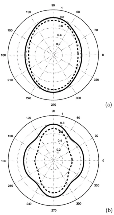
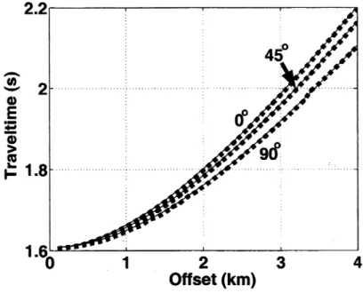
The azimuthal variation of the normalized spreading L~^ at two different offsets is plotted in Figure 2.4. Since the geometrical spreading in our model is symmetric with respect to both vertical coordinate planes, the signature of is repeated in each

quadrant. For the offset equal to the reflector depth, the azimuthal variation of L~^ is

close to elliptical, as predicted by the weaJj-anisotropy approximation (Figure 2.4a). The fractional difference between the values of L~^ in the symmetry planes, which determines the overall magnitude of the azimuthal variation of the inverse geometrical spreading, is about 30%. Hence, for this model the eccentricity of the "geometrical-spreading ellipse" exceeds that of the NMO ellipse (18%). For larger offset-to-depth