How to measure the degree of PIT-ness in a credit rating system for a low default portfolio?

DEGREE PROJECT IN MATHEMATICS, SECOND CYCLE, 30 CREDITS

STOCKHOLM, SWEDEN 2020

How to measure the degree of

PIT-ness in a credit rating system for a

low default portfolio?

An alternative approach using a markovian framework

SIGGE AHLQVIST

MATTEUS ARRIAZA-HULT

How to measure the degree of

PIT-ness in a credit rating

system for a low default

portfolio?

An alternative approach using a markovian framework

SIGGE AHLQVIST

MATTEUS ARRIAZA-HULT

Degree Projects in Financial Mathematics (30 ECTS credits) Master’s Programme in Applied and Computational Mathematics KTH Royal Institute of Technology year 2020

Supervisor at Nordea Bank Abp: Johan Dimitry Supervisor at KTH: Sigrid Källblad Nordin Examiner at KTH: Sigrid Källblad Nordin

TRITA-SCI-GRU 2020:085 MAT-E 2020:048

Royal Institute of Technology School of Engineering Sciences

KTH SCI

SE-100 44 Stockholm, Sweden URL: www.kth.se/sci

Abstract

In order to be compliant with the Basel regulations, banks need to compute two probabilities of default (PDs): point-in-time (PIT) and through-the-cycle (TTC). The aim is to explain fluctuations in the rating system, which are expected to be affected by systematic and idiosyncratic factors. Being able to, in an objective manner, determine whether the rating system is taking the business cycle - i.e the systematic factors - into account when assigning a credit rating to an obligor is useful in order to evaluate PD-models. It is also necessary for banks in order to use their own risk parameters and models instead of standardized models, which is desirable for most banks as it could lower capital requirements.

This thesis propose a new measure for the degree of PIT-ness. This measure aims to be especially useful when examining a low default portfolio. The proposed measure is built on a markovian approach of the credit rating system. In order to find a suitable measure for a low default portfolio, the proposed measure takes into account credit rating migrations, the seasonal component of the business cycle and time series analysis. An analysis were performed between two different credit portfolios in order to interpret results.

The results demonstrated that the degree of PIT-ness was lower in a low default portfolio in comparison with a sampled portfolio which displayed a greater amount of rating migrations with a larger magnitude. The importance of considering relevant macroeconomic variables to represent the business cycle was mentioned amongst the most important factors to consider in order to receive reliable results given the proposed measure.

Keywords

Markov theory, Business cycle, Migration matrix, Directional mobility index, Time series analysis, Spectral analysis, Basel III, PIT-ness, PIT, TTC.

Sammanfattning

För att uppfylla Basel regelverken behöver banker beräkna två sannolikheter för fallissemang (PD): point-in-time (PIT) och through-the-cycle (TTC). Målet är att förklara fluktuationer i betygssystemet, som förväntas påverkas av systematiska och idiosynkratiska faktorer. Att på ett objektivt sätt kunna avgöra om betygssystemet tar hänsyn till affärscykeln dvs de systematiska faktorerna -när man tilldelar en kredittagare ett kreditbetyg är användbart för att utvärdera PD-modeller. Detta är också nödvändigt för att banker ska få använda sina egna riskparametrar och modeller istället för standardiserade modeller, vilket är önskvärt för de flesta banker eftersom det kan sänka kapitalkraven.

Denna avhandling föreslår ett nytt mått för att mäta graden av PIT-ness. Detta mått syftar till att vara särskilt användbart när man utvärderar en kreditportfölj med få fallissemang. Det föreslagna måttet är byggt på en Markov tillämpning på kreditbetygssystemet. För att hitta ett lämpligt mått för en kreditportfölj med få fallissemang, tar det föreslagna måttet hänsyn till kreditbetygsmigrationer, säsongskomponenten i affärscykeln och tidsserieanalys. En analys utfördes mellan två olika kreditportföljer för att tolka resultaten.

Resultaten visade att graden av PIT-ness var lägre i en kreditportfölj med få fallissemang jämfört med en testportfölj som uppvisade en större mängd kreditbetygsmigrationer med en större magnitud. Vikten av att beakta relevanta makroekonomiska variabler för att representera affärscykeln nämndes bland de viktigaste faktorerna att beakta för att få tillförlitliga resultat givet det föreslagna måttet.

Nyckelord

Markov teori, Affärscykel, Migrationsmatris, Riktningsrörelsesindex, Tidsserieanalys, Spektralanalys, Basel III, PIT-ness, PIT, TTC.

Acknowledgements

We would like to thank Nordea’s Credit Risk Model team and especially Johan Dimitry for taking the time to guide us in our work, providing us with materials and added valuable input when requested.

An expression of gratitude towards our academic supervisor at KTH Royal Institute of Technology, Sigrid Källblad. Your interest and willingness to keep discussions going has pushed the work forward.

We would also like to thank family and friends for your encouragement and unconditional support throughout our time at KTH in what marks the end of our studies.

A special thanks to Emil Gnem and André Gerbaulet, whom have spent many long days and nights together with us studying to exams and writings reports.

Contents

2.2.1 Discrete-time Markov Chain . . . 18

2.2.2 Properties of the Markov Chain . . . 18

2.2.3 The cohort model . . . 19

2.3 Directional mobility index . . . 20

2.3.1 Properties of the mobility index . . . 21

2.4 Time series analysis . . . 22

2.4.1 Time series model . . . 22

2.4.2 Additive decomposition . . . 22

2.4.3 Stationarity . . . 23

2.4.4 Stationarity tests . . . 24

2.4.4.1 Augmented Dickey-Fuller test (ADF-test) . . . 24

2.4.4.2 Kwiatkowski-Phillips-Schmidt-Shin (KPSS) test . . 24 2.4.5 Spectral density . . . 25 2.4.5.1 Periodogram . . . 26 2.4.6 Standardization . . . 27 3 Literature review 28 3.1 Previous studies . . . 28

3.1.1 Structural-form models and reduced-form models . . . 28

3.1.2 Measure of the degree of PIT-ness . . . 30

3.1.3 Low default portfolio . . . 31

4 Data 33 4.1 Handling data . . . 33 4.1.1 Credit data . . . 33 4.1.1.1 Non-rated states . . . 36 4.1.1.2 Recovering defaults . . . 36 4.1.1.3 Mapping ratings . . . 37 4.1.1.4 Clustering ratings . . . 37

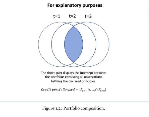
4.1.1.5 Portfolio composition principles . . . 37

4.2 Credit portfolios . . . 38

4.2.1 Low default portfolio . . . 38

4.2.1.1 Data handling, low default portfolio . . . 38

4.2.2 Sampled portfolio . . . 39

4.2.2.1 Data handling, sampled portfolio . . . 39

4.3 Business cycle . . . 40

4.3.1 Unemployment rate . . . 40

4.3.2 Final consumption expenditure (% of GDP) . . . 40

4.3.3 Handling missing data . . . 41

5 Method 42 5.1 The Markov model . . . 42

5.2 Directional mobility index . . . 44

5.2.1 Creating the directional mobility index time series . . . 44

5.3 Determining the business cycle . . . 46

5.3.1 Business cycle estimate - Unemployment rate . . . 47

5.3.2 Business cycle estimate - Final consumption expenditure (% of GDP) . . . 49

5.3.3 Estimating the seasonal component of the business cycle time series . . . 50

5.3.3.1 Determining the frequency using spectral density of business cycle estimates . . . 50

5.3.3.2 Creation of sinusoidal waves representing the seasonal component of business cycle time series . 53 5.4 The measure of the degree of PIT-ness . . . 55 5.4.1 Standardization of time series . . . 55 5.4.2 The measure of the degree of PIT-ness . . . 58

5.4.2.1 The development of the measure of the degree of PIT-ness . . . 58

6 Results 60

6.1 Degree of PIT-ness letting unemployment rate represent the business cycle . . . 60 6.2 Degree of PIT-ness letting final consumption expenditure (% of

GDP) represent the business cycle . . . 61

7 Discussion 62

7.1 Interpretation of results . . . 62 7.2 Conclusions and implications . . . 63 7.3 Suggestions for further studies . . . 69

List of Figures

1.1 Display of the PD of a portfolio depending on the rating philosophy

utilized during different periods of the business cycle. . . 9

1.2 Portfolio composition. . . 11

2.1 Visualization of a business cycle. . . 15

2.2 Decomposition of an additive time series. . . 23

2.3 Example of a periodogram, the y-axis corresponds to the level of spectral density. . . 26

5.1 Example of migration matrices, 2009-2010; Upper: Low default portfolio, Lower: Sampled portfolio. . . 43

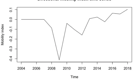
5.2 Directional mobility index time series of the low default portfolio, using v =|i − j| and w = p0(i). . . 45

5.3 Directional mobility index time series of the sampled portfolio, using v =|i − j| and w = p0(i). . . 45

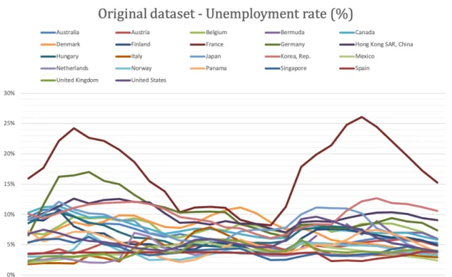
5.4 Original data set - Unemployment rate adjusted to the credit portfolio. 48 5.5 Weighted average Countries - Unemployment rate adjusted to the credit portfolio. . . 48

5.6 Original data set - Final consumption expenditure (% of GDP). . . . 49

5.7 Weighted average Countries - Final consumption expenditure (% of GDP). . . 50

5.8 Periodogram - Unemployment rate adjusted for the credit portfolio. 52 5.9 Periodogram - Final Consumption expenditure (% of GDP) adjusted for the credit portfolio. . . 52

5.10 Sinusoidal business cycle estimate using frequency retrieved from unemployment rate. . . 54

5.11 Sinusoidal business cycle estimate using frequency retrieved from final consumption expenditure (% of GDP). . . 55

5.12 Time series of the standardized directional mobility index of the low default portfolio vs. sinusoidal wave estimate letting Unemployment rate represent the business cycle. . . 56

5.13 Time series of the standardized directional mobility index of the sampled portfolio vs. sinusoidal wave estimate letting

Unemployment rate represent the business cycle. . . 56

5.14 Time series of the standardized directional mobility index of the low default portfolio vs. sinusoidal wave estimate letting Final

consumption expenditure (% of GDP) represent the business cycle. 57

5.15 Time series of the standardized directional mobility index of the sampled portfolio vs. sinusoidal wave estimate letting Final

List of Tables

2.1 Alternative choices of the jump parameter, v. . . 20

4.1 Sample of the original dataset provided by Nordea. . . 34

4.2 S&P credit ratings. . . 35

5.1 The geographical composition of the credit portfolio. . . 46

5.2 Stationarity tests for the business cycle estimates . . . 51

5.3 Frequencies and periods determined from the periodograms for the business cycle representations . . . 53

6.1 Results for the low default portfolio. . . 60

6.2 Results for the sampled portfolio. . . 60

6.3 Results from the low default portfolio. . . 61

1

Introduction

Since the recent economic downturn periods, there has been continuous advancement of the regulatory requirements. Adequate risk mitigation and overall risk management, including quantitative risk modeling, is rapidly evolving and gaining attention from regulators well as the banks. The experience with banking crises in numerous countries has also demonstrated the intricate links between deterioration in creditor quality, macroeconomic conditions, and institutional failure, highlighting the importance of evaluating the credit risk models utilized.

1.1

Background

The major source of risk for banks is the credit risk, being the risk that one of the bank’s counter parties goes into default and thereby not repaying interest and/or principal [6]. A solid framework for measuring credit risk is therefore of the utmost importance for a bank to manage and control its credit risks properly. Since the foundation of the Basel Committee in 1974, the Basel accords have been developed and fine tuned during several occasions until today’s date. The latest implementation with the purpose of enhancing the financial stability is the Basel III accords, whose two main amendments compared to the Basel II accords consists of stricter capital requirements and an introduction of regulatory capital requirements [5]. In order to become compliant with the Basel III frameworks, most financial institutions will have to develop internal models to adequately determine the risk arising from their credit exposures. The amount of risk a bank faces have an impact on the buffer capital the regulatory capital requirement -that banks are required by regulators to put aside as a cushion in case the risks would materialise.

Under the Basel II internal ratings-based approach (IRB), banks are allowed to use their own estimated risk parameters for the purpose of calculating regulatory capital [8]. One of the main elements in doing so under the IRB approach is to determine the probability of default (PD) of their obligors, which is based on the bank’s own assessment of the PD of the individual borrowers [9]. In this

context, banks build up rating systems, which refers to the entire mathematical and technological infrastructure that a bank has put in place to quantify and assign the risk parameters. In order to adopt the IRB approach, banks must also satisfy certain requirements that they can demonstrate to the national supervisor, including a logical and documented methodology for the rating system. This is required for a bank to be allowed to use its internally created ratings systems [22]. The Basel capital requirements regulation also requires banks to take all relevant information into account when assessing an obligor’s default risk [49].

In order to explain the methodology of the rating systems used to the national supervisor under the IRB approach, bank’s seeks to use measures for explanatory and validation purposes. One aspect that bank’s seeks to clarify in their models is to which extent they are depending on the current state of the business cycle. In its latest proposal regarding the IRB approach, the Basel committee of banking supervision states: ”Rating systems should be designed in such a way

that assignments to rating categories generally remain stable over time and throughout business cycles. Migrations from one category to another should generally be due to idiosyncratic or industry-specific changes rather than due to business cycles” [7]. The aim is to explain fluctuations in the rating system,

which are expected to be affected by systematic and idiosyncratic factors. The former factor expresses rating grades that excludes migrations due to the business cycle, which leads to a congruous definition for through-the-cycle (TTC) rating grades. The latter expresses the point-in-time (PIT) rating grades which explains the rating grades that depends on changing macroeconomic conditions.

The two factors, TTC and PIT, are also mentioned in the International Financial Reporting Standard 9 (IFRS9). IFRS9 requires banks to be able to be aware of the rating philosophy of their rating systems and explicitly be able to model

”point-in-time, forward looking PDs”. In order to describe the rating system to a third

party, a measure of how sensitive the rating system’s estimate is to the systematic influence of the business cycle is valuable. This measure is called the degree of point-in-time-ness (PIT-ness) in the rating system. IFRS9 also implicate that an indicator which shows the PIT-ness of the rating system should be used in order to choose the right method for comparative purposes [31]. The information

regarding how a rating system is responding to an economic expansion and an economic recession is therefore highly relevant from this perspective and can also be used for calibration purposes. This document also includes the expectation that banks are aware of the rating philosophy of their rating systems (i.e the level of PIT-ness), given the following statements about the measure of the degree of PIT-ness:

• ”It should be able to analyze the appropriateness of the philosophy

underlying the rating or pool assignment in terms of how institutions assign exposures, obligors or facilities to risk buckets according to appropriate risk drivers”.

• ”It should decide the rating philosophy”.

• ”The choice of rating philosophy must be taken into account in the

calibration”.

• ”Care needs to be taken in the use of information from another rating

system that has a different rating philosophy”.

Intuitively, the degree of PIT-ness is a characteristic of the bank’s rating system that tells us how sensitive the rating system estimates are to the systematic influence of the business cycle. However, matters become more complicated if the bank obtains its PD estimates not directly, but rather in two consecutive steps: first, by assigning rating grades to customers on the basis of the ordinal rating score (i.e rating assignment), and, second, by estimating rating-grade PDs (i.e calibration). In this case an additional dimension of the problem is to be considered, namely rating migration. The latter splits the impact of the business cycle into two parts, so that one can talk about the degree of PIT-ness of a rating system (i.e the degree of rating migration in response to changing macroeconomic conditions) [44]. The approach to be investigated in this thesis uses the credit ratings and its migrations to assess the PIT-ness of the rating system. Credit ratings are set by rating agencies such as Standard and Poor’s (S&P) or Moody’s, but larger banks and financial companies often have their own internal rating system used on its counter parties [52].

As the first contribution in this study, this thesis seeks to estimate rating migrations using a Markovian framework for a low default portfolio, meaning

that an obligors credit rating can be regarded as a Markov chain. This approach requests that the rating system considered uses some sort of ordinal rating scale. The markovian approach is specifically relevant for a low default portfolio due to the fact that such a portfolio consists of few actual default observations. Thus applying structural-form based approaches, that will be presented in greater detail in section 3.1.1, could be problematic. Credit ratings are considered as an evaluation of the credit risk of an obligor and thus provide an implicit forecast of the likelihood of an obligor defaulting [45]. Since a PIT-system re-grades obligors more actively than a TTC-system, the degree of PIT-ness, which provides a measure of the rating philosophy, can be determined by measuring the mobility of transition matrices. The mobility of a transition matrix can be measured by a single number, namely a mobility metric or index. There are two classes of mobility metrics, eigenvalue based metrics and norm based metrics. The eigenvalue based metrics measure the amount of mobility inherent in a particular transition matrix because they can be used to derive the future composition of credit ratings distribution. The norm based metrics measure the distance or magnitude of the change in the current distribution of ratings implied by a particular transition matrix. This thesis seeks to measure the mobility of transition matrices using a norm based metrics. One interpretation is that is also is a measure of the degree of rating migration. Hence, it will be a characteristic of the rating grades, pertaining to the assignment step rather than to a particular calibration technique. Thus, this thesis propose a new way of defining and estimating the degree of PIT-ness of a rating system that will take into account the direction and the magnitude of the credit rating migrations, well as considering the distribution of the obligors’ credit ratings. Furthermore, this thesis seeks to estimate the business cycle. This will be done in order to define how sensitive the rating system is considering the business cycle, which will be important given the measure of the degree of PIT-ness presented in this thesis. By evaluating time series, reflecting the directional mobility of transition matrices and the seasonal component of the estimated business cycle, this thesis aims to provide a new measure, assessing the degree of PIT-ness of a rating system. Consequently, this work can hopefully improve the accuracy of the assessment of credit risk well as being beneficial for all banks with an internal rating system.

1.2

Problem

To adopt the IRB approach and its continued use, a bank must satisfy certain minimum requirements that it can demonstrate to the regulatory supervisor. A rating system refers to the entire mathematical and technological infrastructure a bank has put in place to quantify and assign the risk parameters. Banks are allowed to use multiple ratings systems for different exposures, but the methodology of assigning an exposure to a particular rating system must be logical and documented; banks are not allowed to use a particular rating system to minimize regulatory capital requirements.

According to the Basel Framework, the standard risk weights for credit risks are very conservative compared to the historically observed loss levels. Banks with larger credit portfolios with lower risk usually have a business case of calculating their own risk parameters in their credit risk models, since this will decrease their capital requirements. The relevance for a bank to use its own credit risk model could therefore be inherited from the fact that the demands on capital requirements is based on the credit risk models, either provided by Basel regulations and IFRS9 or by the banks [23]. If the bank could provide an own credit risk model to calculate the capital required that is approved by the national supervisor, the demand on capital requirements could be optimized based on the individual bank’s demands. If a bank finds that it could be valuable for them to optimize their capital allocation, then they would like to create their own credit risk models. For this to be approved, the bank has to cater the national supervisor with a methodology for why they believe that their own risk parameters in their credit risk models could replace the risk parameters in the regulatory capital credit risk model. To grant further relevance to the model created by the bank, measures for how their credit risk models are operating could be used for evaluation. An attempt to create such a measure for evaluation would be to measure the degree of PIT-ness in a rating system. Intuitively, the degree of PIT-ness is a characteristic of the bank’s rating system that tells us how sensitive the rating system is to the systematic influence of the business cycle.

To focus the scope by having clear constraints, an important aspect of the measure is to ensure its feasibility when applied. Hence, the following research question

was posed for this thesis:

How to measure the degree of PIT-ness in a credit rating system for a low default portfolio?

To answer the main research question of this thesis and in order to produce further understanding in the subject, the following sub-questions are identified as:

• How is a business cycle determined, what are relevant macroeconomic factors to consider?

• How should the credit portfolio evaluated be taken into account?

• How is it made sure that the measure provides a link between the rating system and the business cycle?

• How is the degree of PIT-ness interpreted given the proposed measure?

1.3

Purpose

This study aims to investigate to which degree a rating system using an ordinal rating scale is considering the business cycle when determining the ratings of its obligors. Since this thesis intends to investigate a low default portfolio, the objective specifically aims to provide a measure that can simplify the degree of PIT-ness in such portfolios that generally are more complicated evaluating with other approaches, such as structural-based approaches.

1.4

Goal

The goal is to find a measure that can be used for any financial institute assigning ordinal credit ratings to their obligors in order to determine whether their rating system is taking into consideration the business cycle when determining the ratings. Under this approach, banks are assumed using hybrid rating system, adjusted to both PIT and TTC methodologies when assigning their obligors credit ratings.

The measure proposed has a number of features and seeks to fulfill the Insititute of International Finance (IIF) requests for a measure of the degree of PIT-ness [42] :

• The measure should be able to compare rating systems independently

from the portfolio it is measured on. Therefore, the measure should

not be influenced by the portfolio composition (e.g with different rating distributions or different default rates).

• The measure should also not be influenced by changes in the portfolio

composition (e.g exits, new borrowers).

• The measure should have a floor and a ceiling.

• The measure should include a link between macro economy and the rating

(or PD) development. The default rate could be one indicator for the macro economy.

• In case of a stable macro economy, the measure should not be defined (or

zero). As then, one could not be able to distinguish between a PIT or a TTC rating system.

• A rating system which reacts faster and in the right direction to the changes

in the macro economy should get a higher value.

• The measure should not be influenced by the accuracy of the rating system.

1.4.1 Expected contribution

With IFRS 9 recently being implemented as of January 2018, and Basel IV being implemented continuously until 2027, many studies have been presented during the past decade on the topic of macroeconomic factors in relation to credit risk evaluation and the measure of the degree of PIT-ness; see e.g [23]. However, the focus on the macroeconomic impact on the credit risk of low default portfolios, and the evaluation of the measure of PIT-ness in the rating systems utilized, is found to be limited in previous studies. Especially, research concerning low default portfolios has not been identified by the authors in scientific publications. Also, studies that seeks to evaluate the degree of PIT-ness of rating systems which make use of structural-form models might not be favorable for low default portfolios. By using a markovian approach in order to define a measure on the degree of PIT-ness, this thesis specifically seeks to provide a new method of evaluating low default portfolios principally.

risk modeling teams with the need to assess their credit risk exposure well as for consultants. It will provide the credit risk modeling team with analysis about the assessments and determination of the important terms of the relationship between macroeconomic factors and the PIT-ness of their rating systems. The benefit of a better credit risk assessment is twofold. First it gives banks a better control over the risks they are facing and can be a support for business decisions. Secondly, internal models typically results in lower risk measures and thereby lower capital requirements. Since capital is costly, this is a direct benefit for a bank. As the study is principally focusing on a low default portfolio analysis, it aims to make use of relationships and theories concerning rating systems in relation to the macro economy and apply it to a quantitative analysis on the rating migrations of these low default obligors.

1.5

Methodology

In order to define a measure for the degree of PIT-ness in a credit rating system for a low default portfolio, the following methods are adopted. To measure to which extent the rating system is considering the business cycle, the business cycle had to be defined. The approach used in this thesis to define the business cycle is based on creating time series of different macroeconomic variables that could be used to represent a business cycle, such as Final consumption expenditure (% of GDP) and Unemployment rate. Specifically, the seasonal component of the business cycle is of certain interest, as it could reflect the cyclicality in the business cycle time series considered. The seasonal component of the business cycle time series is then interpreted as the reference time series displaying 100% PIT-ness.

Generally, rating systems are built as a combination of PIT and TTC rating philosophies. A PIT rating philosophy account for the current macroeconomic factors, and as a result, such a rating philosophy will closely track the business cycle. A TTC rating philosophy accounts only for the idiosyncratic factors, and as a result, a rating system applying a TTC philosophy will not change largely due to changes in the macro economy. The TTC-part of the rating philosophy is, just as the name gives the hint of, some sort of stable value through at least one business cycle. To increase the accuracy of the measure of the degree of PIT-ness, a long

time series is coveted. Although, given this approach, most importantly was that the time series created ran through at least one business cycle.

Figure 1.1: Display of the PD of a portfolio depending on the rating philosophy utilized during different periods of the business cycle.

The aim is to be able to model an arbitrary rating system using an ordinal scale and to put this into relation with the seasonal component of the business cycle to determine the degree of PIT-ness. In order to do so, this thesis make use of Markov theory and migration matrices to determine the mobility of the rating system. This is done by identifying obligors credit rating migrations as Markov chains, fulfilling the Markov property. By calculating the transition probabilities with a cohort approach, the migration matrix between two measure points is decided, making it possible to evaluate the dynamics of the migration matrix using a directional mobility index. Creating a time series of the values provided by the directional mobility index enables further evaluation. By examining the relationship between the standardized seasonal component of the business cycle time series and the standardized directional mobility index time series, this thesis hope to describe the degree of PIT-ness of the rating system. In order to simplify the interpretation of the results for the low default portfolio, a sampled portfolio is created. The degree of PIT-ness is also computed for this portfolio and compared to the results for the low default portfolio.

1.6

Limitations

The main focus on the study is to design a measure that provides a link between the business cycle and the rating system to be able to determine the degree of PIT-ness in the rating system. This thesis is limited to studying credit rating migrations, Markov theory and time series analysis.

The study was limited to generated data with ratings of banks in a low default portfolio. The data are generated to mimic S&Ps described rating methodology. Macroeconomic data was sourced from The World Bank. Hence market behaviors were expected to differ across countries, so was the macro economy. To conduct this study, an evaluation of the credit portfolio had to be performed in order to provide an appropriate link between the rating system and the macroeconomic conditions. The macroeconomic factors utilized in this thesis have been given on a country-specific level, which might not be representative for the ingoing obligors in the credit portfolio as they specifically represents one business sector.

As mentioned in section 1.4, the measure proposed in this paper search to fulfill IIFs requests for a measure of the degree of PIT-ness, which required some limitations for the proposed measure [42].

• The measure should be able to compare rating systems independently

from the portfolio it is measured on. Therefore, the measure should

not be influenced by the portfolio composition (e.g with different rating distributions or different default rates).

This measure was developed using a markovian approach that made use of the ratings set using an ordinal rating scale. This is the commonly used manner for both rating institutes and bank’s internal methods to assign their obligor’s with a credit rating. The approach presented is flexible in using different ordinal ratings scales in order to calculate PIT-ness. Regarding the portfolio composition, principles are defined, which are mentioned in the following request.

• The measure should also not be influenced by changes in the portfolio

composition (e.g exits, new borrowers).

composition. These are the following:

– Obligors must have been assigned ratings throughout the full business

cycle.

– Obligors that will be used when computing the transition matrices must

have non-defaulted rating grades throughout the full business cycle.

Figure 1.2: Portfolio composition.

• The measure should have a floor and a ceiling

This request was solved by introducing a quotient in the measure of the degree of PIT-ness. Given that the measure introduced will equal 1, it will suggest that that the rating system is 100% PIT. If the measure instead equals 0, it will suggest that the rating system is 0% PIT.

• The measure should include a link between macro economy and the rating

(or PD) development. The default rate could be one indicator for the macro economy.

The directional mobility index, on which the time series of investigation is based on, includes a sign-function that will assign rating downgrades with a negative value and assign rating upgrades with a positive sign. S&Ps

credit ratings express a forward-looking opinion about the capacity and willingness of an entity to meet its financial commitments as they come due. But also the credit quality of an individual debt issue, such as a corporate or municipal bond, and the relative likelihood that the issue may default [46]. By reviewing credit rating migrations for individual obligors only, one could not tell whether this would be due to idiosyncratic factors or if it is due to systematic factors. As the number of obligors increase, the idiosyncratic factors that affects the credit ratings migrations of the different obligors will subsequently take each other out and one will only be left with the systematic factor that affects credit rating migrations. Hence credit ratings and credit ratings migrations are providing information regarding the business cycle. The approach and the measure presented in this thesis will therefore include a link between macro economy and the rating development.

• In case of a stable macro economy, the measure should not be defined (or

zero). As then, one could not be able to distinguish between a PIT or a TTC rating system.

The measure proposed in this thesis make use of an estimate of the seasonal component of the business cycle during at least one business cycle. The measure requires not just a single observation in order to be computed. Therefore, a stable macro economy would in this thesis refer to the estimate of the seasonal component of the business cycle being flat throughout the examined period of time. The proposed measure in this thesis make use of a min-max normalization to be able to compare the directional mobility index time series and the time series representing the seasonal component of the business cycle. Given that the time series are normalized on the interval [0, 1], a flat time series would not be defined due to singularity. Consequently, the measure is not defined in case of a stable macro economy, whereas it would not be possible to distinguish between a PIT or a TTC rating system.

• A rating system which reacts faster and in the right direction to the changes

in the macro economy should get a higher value.

The measure presented is based on a directional mobility index that includes a jump condition and weight condition. The jump condition will emphasize

major changes in credit rating grades, giving these a larger magnitude in the calculations of the directional mobility index. The weight condition will reflect the effort required of making transitions between different rating grades based on the starting rating grade.

• The measure should not be influenced by the accuracy of the rating system. This part of IIFs requests will be outside of the scope of this thesis as external data are used from S&P in order to calculate the transition matrices. Credit ratings are generally set by rating agencies such as Standard and Poor’s or Moody’s, but larger banks and financial companies often have their own internal rating system for its counter parties. There is the possibility to construct own rating buckets and PD estimates in order to create own rating grade outcomes. Due to the fact that this thesis has a time limit, and this part would require extensive work that could be prohibitive, it was decided to use the ratings provided by S&P. Hence, this thesis will not try to determine the accuracy of their rating system and in order to fulfill the requests given by IIF fully, the creation of self-made rating buckets for example, would be necessary.

2

Theoretical background

In this chapter, the relevant background and related theory is presented to give context to the analysis.

2.1

Business cycle

There is no universal method of defining the length of a business cycle, according to Burns and Mitchell [14] it can be described as follows:

”Business cycles are a type of varying rotations that can be found in aggregated economic activity of nations that organize their work mainly in business enterprises: a cycle consists of expansions occurring at about the same time in many economic activities, followed by similarly general recessions, contractions and revivals which merge into the expansion phase of the next cycle; this sequence of changes is recurrent but not periodic; in duration business cycles vary from more than one year to ten or twelve years; they are not divisible into shorter cycles of similar character with amplitudes approximating their own”.

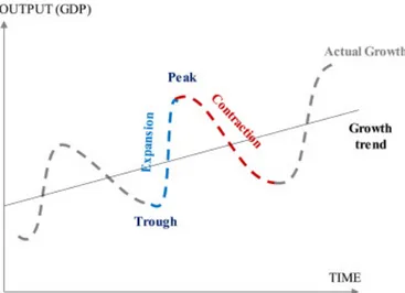
Given this definition, one can identify four distinct phases of a business cycle; trough, expansion, peak and contraction. Luvsannyam et al. [39] describes the characteristics of the different phases accordingly; through is the turning point when the contraction transforms into the expansion phase and the peak is the turning point when the expansion phase transforms into the contraction phase.

Figure 2.1: Visualization of a business cycle.

Petrov & Rubstov [44] presents different methods in order to estimate the business cycle. They mention that one can obtain an estimate of the business cycle by conditioning rating transition probabilities on macroeconomic variables. In their work, they proclaim that some requirements has to be fulfilled to be able to estimate a business cycle. Amongst these are the following:

• It must be external - otherwise it will be incorrect to base both estimation

and validation on the same data.

• The data needs to be forecastable.

• The actual numbers, not just the forecasts, must be observable.

• The length of the time-series used should be long enough to capture an

economic downturn period.

Petrov & Rubstov clarifies that there are many data sets that could potentially satisfy these requirements. They argue that typically, macroeconomic indexes closely followed by the financial market, such as GDP growth or inflation, are of interest.

2.2

Markov theory

In this section, definitions, properties and aspects of the Markov chain theory utilized in this thesis are presented in accordance with the works of Enger and Grandell [21].

Observations of an event that is suspected to be in-part randomly driven, can at each discrete point in time t ∈ T be mathematically described by a stochastic variable X(t). Moreover, the chain of events can be described by a discrete time stochastic process. In this thesis the discrete time stochastic processes known as Markov chains are of special interest.

Definition 1: A family of stochastic variables{X(t); t ∈ T }, where T ∈ [0, ∞) is

the index set of a the process, is called a discrete stochastic process.

In order to define the Markov chain, the Markov property has to be defined first. It is defined as:

Definition 2: A stationary, discrete Markov chain is satisfying the Markov

property if for all stages n and all states x0, x1, ..., xn+1,

P (Xn+1 = xn+1|X0 = x0, X1 = x1, . . . , Xn= xn) = P (Xn+1 = xn+1|Xn = xn).

Explicitly, the stochastic process at stage n + 1 is only dependent on its value at stage n.

Furthermore, the Markov chain can shift between different states. The set that considers all different states that the Markov chain can move between is referred to as the state space. It is defined as follows:

Definition 3: A finite or countable set S forms the state space of a Markov chain.

I.e each possible outcome xi ∈ S is called a state and the set of possible outcomes

is defined as Xi.

Given this, the Markov chain can be defined as:

Definition 4: A Markov chain is a stochastic process,{Xi}i>0, with a sequence

of stochastic variables with outcomes x0, x1,... on the set S that satisfies the

Due to the Markov property, the Markov chain is often referred to as being ”memory-less”. Furthermore, given that the Markov chain is defined, other concepts that are related with the Markov chain can subsequently be defined. One of these is the transition probability which is defined as:

Definition 5: The transition probability, pij, in a time-homogeneous Markov

chain is defined as,

pij = P (Xn= j|Xn−1 = i), (1)

i.e the probability to go from state i to j in one time step.

The matrix that is constructed by all possible transition probabilities is defined as the transition matrix. The transition matrix has the following properties:

Definition 6: The transition matrix, P, is defined as the matrix (pij)ij ∈ S which

consists of transition probabilities such as:

P =        p11 p12 p13 . . . p21 p22 p23 . . . p31 p32 p33 . . . .. . ... ... . ..        . (2)

Theorem 1: (Properties of the transition matrix)

a) ∑n_j=1pij = 1for i = 1, . . . , n.

b) pij ≥ 0, ∀i, j = 1, 2, . . . , n.

The concept of stationarity is of interest when studying Markov processes in order to define under which circumstances the distribution of X(t) is converging, and when the limit distribution is independent of the starting state.

Definition 7: A distribution, π = (π0, π1, ...), is a stationary distribution to a

Markov chain with the corresponding transition matrix P if:

This is sometimes referred to as time-homogeneity, which imply to the definition of the Markov chain that,

P (Xn+1= a|Xn= b) = P (Xn= a|Xn−1= b).

2.2.1 Discrete-time Markov Chain

In this thesis, the Markov chain in discrete time will be utilized. I.e each time step can be counted as a natural number 0, 1, 2, .. in which each stochastic process has its outcomes within a finite state space, S={ik, k = 1, 2, ..., N }. Worth mentioning

is that the time step ∆tkis constant, well as the time settings in the Markov chain

are referred to as stages.

2.2.2 Properties of the Markov Chain

Markov chains has some special properties that will be defined in the upcoming section.

Accessibility: A state j is said to be accessible if there is a non-zero probability

eventually moving to this state for a system starting in state i.

Communication: A state i is said to lead to state j if it is possible to go from i

to j in zero, one or several time steps, it is denoted i → j. Two states are said to communicate if i→ j and j → j, it is denoted i ↔ j.

Irreducibility: A set of states which are communicating with each other is called

an irreducible set of states. A chain for which its state space is irreducible is called a irreducible chain.

Transiency: In a Markov chain, a state i is said to be transient if there is a

non-zero probability that the Markov chain will never return to state i. A state is said to be recurrent if it is not transient.

Absorbing: A state i lead to state j if it is possible to in a finite amount of time

steps get from i to j. A state is absorbing if the chain always remains in the state. This means that i is a absorbing state if and only if pii= 1.

Periodicity: Let Di be the set of integers n such that it is possible to from state

i return to this state in n time steps. The period, di, is referred to as the greatest

common divider to the integers in Di. If di = 1, it is called an aperiodic state.

2.2.3 The cohort model

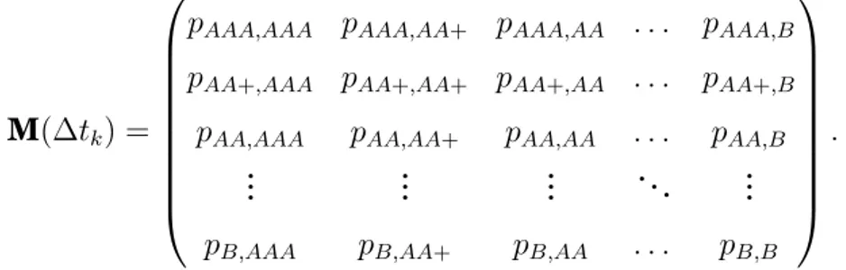
The cohort model can be applied in order to compute the transition probabilities for all possible transition given a specified set S. The transition probabilities can be utilized in order to create a migration matrix M(∆tk), as they constitute

the indexes in this. Migration matrices can for example be utilized to describe transition probabilities for several obligors’ credit rating migrations given one time step.

Let t0, t1, . . . , tnbe discrete time points such that the arbitrary time interval

tk+1− tk = ∆tk, and ∆tk is constant. The estimator of pij(tk)over a time interval

is then, ˆ pij(tk) = Nij(∆tk) Ni(tk) , (3)

where Ni(tk)is the number of obligors in state i at time tk. The factor, Nij(∆tk),

refers to the number of obligors that have migrated from state i to state j between time tkand tk+1[27].

The estimations of pii and pij, form the migration matrix M(∆tk) for the time

interval ∆tk. There is no time-homogeneity assumption, meaning that different

migration matrices will be computed for every ∆tk throughout the business

2.3

Directional mobility index

LetP bet the set of transition matrices:

P = {P = (pij)∈ Rk×k|pij ≥ 0,

k

∑

j=1

pij = 1,∀i = 1, . . . , k}.

A directional mobility index can be defined as a function, I : P → R, chosen in order to provide a suitable and synthetic description of the mobility. It can be utilized in order to evaluate the prevailing direction of the dynamics in the migration matrix. Ferratti et al. [24] presents a directional mobility index originating from a migration matrix, which is the one that is utilized in this thesis. The proposed directional mobility index is defined as follows:

Idir(P ) = n ∑ i=1 wi ∑ j pijsign(i− j)v(|i − j|), (4)

where the function sign is defined as:

sign(x) :=            −1, if x < 0 0, if x = 0 1, if x > 0.

The sign function is supposed to give an indication whether the migration is to a positive or negative direction within the matrix. In their proposed directional mobility index, the initial states are weighted by the factor, wi, for every initial

state i ∈ {1, ..., k} such that wi > 0 and

∑n

i=1wi = 1. In their proposal,

wi corresponds to the percentage of obligors starting from i. The parameter v,

denoted as the jump parameter, estimates the magnitude of the credit rating migrations from state i to state j, for each i, j = 1, . . . , k. It can be assigned in multiple ways, and in their work, Feretti & Ganugi [24] presents the following alternatives for v.

1, log10(|i − j| + 1),

√

|i − j|, |i − j|, |i − j|2_{, e}|i−j|_{− 1.}

As an illustration, selecting v as v = |i − j|, a migration from state i to state

i + 2would be given twice the magnitude in the directional mobility index as a

migration from state i to state i + 1. Linear measures, such as v = |i − j|, are generally a reasonable choice when the variable under study is qualitative, which is the case when evaluating credit rating migrations [25]. Though, the selection of

vis strictly related to the specific dynamics of the variable evaluated.

2.3.1 Properties of the mobility index

The directional mobility index fulfills four important properties; boundedness,

perfect mobility, immobility and monotonicity. The following propositions are

presented in order and will provide the validity of these properties for the family of directional mobility indexes, including the one presented by Ferratti et al.

Proposition 1 For every choice of wi and v, and for every P ∈ P we have,

m1 ≤ Idir(P )≤ m2,

where m1 ≤ 0 and m2 ≥ 0 are not depending on P and defined by:

m1 = n ∑ i=1 wiv(1− i); m2 = n ∑ i=1 wiv(n− i).

Proposition 2 For every choice of wiand v the index, Idir, satisfies Idir(P ) = m1,

if and only if, P = P₋ (perfect positive mobility) and Idir(P ) = m2, if and only

if, P = P+ (perfect negative mobility). Then the index is said to be strongly

perfect mobile.

Proposition 3 The directional index Idirsatisfies the following properties:

a) if wi = 1_nfor every i = 1, . . . , n and P is a symmetric matrix, then Idir(P ) = 0.

b) for every choice of w, if P is a matrix such that for every i = 1, . . . , n and

for every l = i− 1, . . . , n − i it holds pii−l = pii+l, then Idir(P ) = 0.

In this sense Idir(P )satisfies the weak immobility.

Proposition 4 For every P, Q∈ P such that pij ≤ qij, and for every choice of wi

2.4

Time series analysis

A time series is a set of observations{xt}, each one being recorded at a specific

time t. A discrete-time time series is one, in which the set T0 of times at which

observations are made is a discrete set [13]. In this thesis, time series models for the discrete case are evaluated.

2.4.1 Time series model

Definition 8: A time series model for the observed data{xt} is a specification

of the joint distributions (or possibly only the means and covariances) of a

sequence of random variables{Xt} of which {xt} is postulated to be a realization

[13].

A time series model is a dynamic system that is identified to fit a given signal or time series data. Modeling a time series can for example make it easier to identify patterns in the examined data set.

2.4.2 Additive decomposition

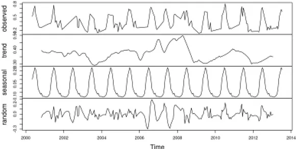
Decomposing time series is a statistical task that refers to the deconstruction of a time series into several components, each representing an underlying category of patterns. An additive decomposition of a time series is illustrated as follows,

Xt= mt+ st+ ϵt, (5)

where mtis the trend component, stis the seasonal component and ϵtis a random

noise term with zero mean [13]. The additive method is often utilized when the seasonal variation is relatively constant over time, i.e, the tendency of the data repeat itself of every L period [35].

Figure 2.2: Decomposition of an additive time series.

2.4.3 Stationarity

A time series,{Xt, t = 0,±1, ...}, is said to be stationary if its statistical properties

is similar to those of the ”time-shifted” time series{Xt+h, t = 0,±1, ...} for each

integer h [13]. Limited attention will be given to those properties that depend only on the first- and second-order moments of{Xt} in this thesis. Based on this, the

following definitions are presented.

Definition 9: Let{Xt} be a time series with E[Xt2] <∞, then the mean function

of {Xt} is µX(t) = E[Xt]. The covariance function of {Xt} is γX(r, s) =

Cov(Xr, Xs) = E[(Xr− E[Xr])(Xs− E[Xs])]for all integers r and s.

Definition 10:{Xt} is (weakly) stationary if

(i) µX(t)is independent of t.

2.4.4 Stationarity tests

There are different tests to determine whether a time series is stationary or non-stationary.

2.4.4.1 Augmented Dickey-Fuller test (ADF-test)

The augmented Dickey-Fuller tests, examines the null hypothesis that a unit root is present in a time series sample. The test starts with a hypothesis test for an auto-regressive (AR) time series, which refers to a time series model that uses observations from previous time steps as input to a regression equation to predict the value at the next time step. The ADF-test is conducted accordingly:

• Xt= ϕXt−1+ ϵt; H0 : ϕ = 1, H1 : ϕ≤ 1, (∗)

where, if H0is true then the time series is said to be non-stationary.

If Xt−1is subtracted from both left-hand side and right-hand side of the equation,

one receives:

• Xt− Xt−1 = (ϕ− 1)Xt−1+ ϵt, and set (ϕ− 1) = δ.

• ∆Xt= δXt−1+ ϵ; H0 : ϕ = 1, H1 : ϕ≤ 1.

If H0 is true, then the time series is said to be non-stationary.

By using the t-ratio, τ = δ ˆ

SE(δ), the augmented Dickey-Fuller test rejects the null

hypothesis of a unit root at significance level ρ (often 0.05). If τ < tρ, the time

series is said to be stationary. This can also be done on a general level for an AR(p) model.

2.4.4.2 Kwiatkowski-Phillips-Schmidt-Shin (KPSS) test

The Kwiatkowski-Phillips-Schmidt-Shin test, examines the stationarity of a time series model. The procedure is similar to the ADF-test, as the null hypothesis

H0 : ϕ = 1is tested against the hypothesis H1 : ϕ ≤ 1. Unlike the ADF-test, the

KPSS-test takes into consideration a trend component mtin the right-hand side

2.4.5 Spectral density

Any signal that can be represented as a variable that varies in time has a corresponding frequency spectrum, which can be calculated using the Fourier transform. The Fourier transform decomposes a function (often a function of time) into its constituent frequencies that can be characterized by cosines and sines. The spectral representation of a stationary time series,{Xt}, is the essential

method to decompose {Xt} into a sum of sinusoidal components with random

coefficients that are uncorrelated, in order to analyze the time series in the frequency domain. Hence, spectral decomposition is an equivalent method for evaluating stationary processes of the Fourier transform.

Given that{Xt} is a zero-mean stationary time series with autocovariance function

(ACVF) γ(·), satisfying ∑∞_h=−∞|γ(h)| < ∞, the spectral density of {Xt} is the

function f (·) defined by [13], f (λ) = 1 2π ∞ ∑ h=−∞ e−ihλ,−∞ < λ < ∞, (6)

where eiλ _{= cos(λ) + isin(λ)and i =}√−1. The summability of |γ(·)| implies that

the series converges absolutely. Both cos and sin have the period 2π, which implies that it is sufficient to confine f (·) to the interval (−π, π]. Some basic properties of

f (·) are:

a) f is even, i.e, f (λ) = f (−λ). b) f (λ)≥ 0 ∀λ ∈ (−π, π].

c) γ(k) =∫_−ππ eikλf (λ)dλ =∫_−ππ cos(kλ)f (λ)dλ.

Definition 11: A function f (·) is the spectral density of a stationary time series

{Xt} with ACVF, γ(·), if

i) f (λ) ≥ 0 ∀λ ∈ (0, π].

ii) γ(h) =∫_−ππ eihλf (λ)dλ for all integers h.

Its frequency, f , can be described as the amount of waves that pass a fixed location in a certain time. The relation between the period, T , and the frequency is defined as T = 1

f. In finance, spectral analysis are especially relevant to processes that

can also be used in order to determine whether there are any dominant cyclical components contained in a time series,{Xt}. Kamen et al. [36] defines the term,

”dominant”, as any sinusoidal component whose amplitude in{Xt} is much larger

than the amplitudes of most of the other sinusoidal components included in{Xt}.

The dominant sinusoidal component is of interest if one would like to represent the cyclical component in a time series given only one sinusoidal component.

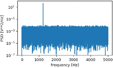
2.4.5.1 Periodogram

A periodogram is a method for estimating the spectral density of a time series. The periodogram can be utilized in order to receive an easy to understand illustration for which frequencies that are dominant in a time series.

Figure 2.3: Example of a periodogram, the y-axis corresponds to the level of spectral density.

If{Xt} is a stationary time series with the corresponding ACVF γ(·) and spectral

density f (·), then the periodogram, In(·), can be regarded as a sample analogue of

2πf (·). The periodogram of {x1, x2, . . . , xn} is given as [13]:

In(λ) = 1 n| n ∑ t=1 xte−itλ|2.

2.4.6 Standardization

Feature scaling is a method used to normalize the range of independent variables or features of data. One such method is the min-max normalization. The method provides a linear transformation of the original range of the data. The technique can be used to fit the data on a predefined boundary. The original formula on the arbitrary interval [a, b] is given as:

x′ = a + (x− xmin)(b− a)

xmax− xmin

. (7)

For the interval [0, 1], the formula is given by:

x′ = x− xmin

xmax− xmin

3

Literature review

This chapter presents relevant literature aided to deepen the knowledge on the topics treated in the thesis. Previous studies within the field of credit risk related to the application of Markov chains in credit-risk-modeling, measures of the degree of PIT-ness well as studies covering the special case regarding low default portfolios are presented.

3.1

Previous studies

3.1.1 Structural-form models and reduced-form models

The credit risk models built by banks can generally be grouped into two main categories: the structural-form models and the reduced-form models. The difference between these two categories of models is the implicit assumption they make about managerial decisions regarding their capital structure. The structural-form models are also called the asset value models for assessing credit risk, typically of a corporation’s debt. These models are generally based on the principle of pricing option in the Black-Scholes model and a more detailed model developed by Merton [12][40]. The Merton model uses the Black-Scholes-Merton option pricing methods and is called structural as it provides a relationship between the default risk and the capital structure of the firm. In spite of the extensions of Merton’s original framework, these models still suffer some drawbacks. As the firm’s value is not a tradable asset, nor is it easily observed, the parameters of the structural form models are difficult to estimate consistently. Also, there are some inclusions of some frictions like tax shields and liquidation costs. Another drawback is that corporate bonds undergo credit downgrades before they actually undergo default, but structural form models cannot incorporate these credit-rating changes. Reduced form models attempt to overcome these shortcomings of structural form models; unlike structural form models, reduced form model make no assumptions at all about the capital structure of the borrowers. In contrast, reduced form models can extract credit risks from the actual market data and are not dependent on asset value and leverage.

3.1.1.1 Markovian approach and transition matrices

There is one strand of the credit-risk-modeling literature that makes use of a matrix of transition probabilities to explain the migration of creditor quality, as measured by proxies such as credit ratings. These reduced-form models, based on rating migrations show the evolution of creditor quality for broad groups of obligors with the same approximate likelihood of default. This approach utilizes matrices of transition probabilities that can be used as an input to model credit evolution, which summarizes a broad range of possible creditor dynamics in a simple and coherent fashion.

Papers such as the one written by Jafry and Schuermann [33] suggested different approaches of comparing credit migration matrices to each other. In their seminal work on credit spread, Jarrow et al. derived the risk premium for the credit risk process from a Markov chain on a finite state space. In this paper, the estimation of PD were derived from transition matrices given a Markov chain [34]. There are also some attempts to identify the impact of the business cycle using rating transition matrices. The works of Wilson [11], Belkin et al. [10], Alessandrini [1], Kim [37], Nickell et al. [41] tried to identify the relationship between the business cycle and rating transition matrices. Rikkers and Thibeault [43] concluded in their studies that capital requirements under a PIT rating method are on average lower than under a TTC rating approach, even if the average PD over the period is the same. However, this study concluded that PIT ratings lead to very volatile and procyclical capital requirements. Cesaroni [16] showed that ex-post PD smoothing is able to remove business cycle effects on the credit risk estimates and to produce a mitigation of obligors’ migration among risk grades over time. This research also concluded that rating scale choice also has a significant impact on rating stability.

Against this convenience of adopting a markovian approach in credit risk modeling is mounting evidence of non-markovian behavior of the rating process. Altman and Kao [3], Carty and Fons [15], Altman [2], Nickell et al., Bangia et al. [4], Lando and Skødeberg [38], Hamilton and Cantor [30] have shown the presence of non-markovian behavior such as ratings drift and industry heterogeneity, and time variation due in particular to the business cycle.

Christensen et al. [18] considered the possibility of latent ”excited” states for certain downgrades in an effort to address serial correlation of ratings changes. Giampieri et al. [28] made use of a hidden Markov model to deduce the state of the economy from rating dynamics although their model focuses specifically on default prediction. Stefanescu et al. [48] considered a simulation-based Bayesian approach that allowed for some ratings momentum. Feretti et al. [24] applied an extension of a Markov chain model, the Mover-Stayer model, in order to determine the migration risk of small and medium enterprises. They found that banks are over-estimating their credit risk resulting in excessive regulatory capital, reinforcing the importance for banks to have well functioning credit risk models in order to be profitable.

3.1.2 Measure of the degree of PIT-ness

There are previous studies proposing different measures of the degree of PIT-ness. In their paper, Petrov & Rubtsov [44], suggests a decomposition of portfolio-level default rates into three components; a TTC-part, a PIT-part and a part that accounts for the natural improvement in portfolio quality due to defaults of the worst obligors. These three components are then obtained for every year in the bank’s historical sample and the degree of PIT-ness is proposed to be:

Degree of PIT-ness = Std dev.(∆ADFP IT)

Std dev.(∆ADFP IT) + Std dev.(∆ADFT T C)

.

The PIT component reflects the standard deviation of the change in the portfolio distribution due to credit rating grade migration, assuming constant default rates per credit rating grade. The TTC component reflects the standard deviation of the change in default rates per credit rating grade assuming no migration.

Another proposal for the degree of PIT-ness was presented by the Italian financial industry risk managers association (AIFIRM) [20], and analyzes the rating models capacity to attribute the volatility of the overall default rate to class migrations. In this proposal, the volatility of the default rate is divided into two components; the volatility of default rate for each credit rating class adjusted for the class migrations, and the overall volatility of the default rate. The relative weight

between these two components is the sought property of the rating system, for which the suggested degree of PIT-ness is defined as follows:

Degree of PIT-ness = Std dev of the default rate adjusted for the class migrations

Std dev. of the default rate .

Jafry & Schuermann [33] proposed a mobility index to calculate the degree of PIT-ness by evaluating transition matrices. In their proposal, the index used is calculated as the Euclidean distance between an observed transition matrix and the time homogenous transition matrix. The homogenous transition matrix is the identity matrix where the ratings do not change with time. Given an observed transition matrix T , a mobility matrix ˆT is defined as:

ˆ

T = T − I,

where ˆT, defines the degree of concentration of the transition matrix along its diagonal that deviates from an identity matrix. The larger the probability of transitioning to a different rating, the less concentrated will the transition matrix be along its diagonal. The average single value of a transition matrix is given by

MSV Dand is defined as:

MSV D =

∑N i=1λi( ˆT

T_{T )ˆ}

N .

In this proposal, λi is the i:th eigenvalue of ˆTTTˆ and N is the dimension of the

mobility matrix. A higher value of MSV D is suggesting a higher probability of

transitioning to a different rating in the rating system.

3.1.3 Low default portfolio

A substantial issue arises in certain credit portfolios consisting of low default obligors, as for higher rating classes practically no defaults are observed, yielding default probabilities of zero. Merton’s model, that uses actual default frequencies (ADF) to calculate the PD will not be effective. A second relevant question relates to the estimation of rating migration risk for the banks’ economic capital: to be effective, internal rating models should be designed coherently not only with the actual borrowers’ standing, but also with their expected assessment pattern [26]. Wilson [53] displayed that transition probabilities change over time as

the state of the economy evolves. In his approach, default probabilities were a function of macro variables such as unemployment, interest rate, the growth rate, government expenses, and foreign exchange rates. Wilson then used macro variables in order to derive the business cycle. The Basel Committee on Banking Supervision also emphasizes the importance of the business cycle, which may improve the accurate assessments of credit risk [6].

4

Data

In this chapter, the data sets utilized are presented and the process of handling data will be described. The process of adjusting the original data in order to establish a final data set will also be described in greater detail.

4.1

Handling data

The data set in its original form contained 11625 observations from 964 obligors, distributed over the years 1980− 2018. The original data set did not contain any missing values. The sections below describes for which reason the original data set was adjusted and how this was executed.

4.1.1 Credit data

The original data set consisted of credit ratings retrieved from an internal database at Nordea in the beginning of each year. The credit ratings were set in a way that mimic how S&P would rate the customers in accordance with their described rating process [47]: ”For corporate, government, and financial

services company or entity (collectively referred to as “C&G”) Credit Ratings, the analysis generally includes historical and projected financial information, industry and/or economic data, peer comparisons, and details on planned financing’s. In addition, the analysis is based on qualitative factors, such as the institutional or governance framework, the financial strategy of the rated entity and, generally, the experience and credibility of management”.