Alternate scale representation of atmospheric energy spectra, An

An Alternate Scale Representation of Atmospheric Energy

Spectra

BY

Ferdinand Baer

Department of Atmospheric Science

Colorado State University

lirprintecl iron1 J O [ : K S A L O F .ITAIOSPHKRIC SCIENCES, 1-01. 19. KO. 4. May 1972, pp. 649-664 ;in~rricnn .\Ietvor~~logici{l SocicLy

1'rintt.d in U. S. ;I.

An Alternate Scale Representation of Atmospheric Energy Spectra

L)cp/. JJ :11111o~pl1t~ric Science, C)ldrudo .>'toie L:r~ir c r ~ i i y , ].'or/ C;~liilr,

c \l+nuscript received i Septcinber 1971)

:ilthoagh it is known that 311 rpati:rl scitles arc nonlinearly interrelated in any prediction model of the atn~c~sl)lic~-c, truncation demands a limit to scale resolution. One is therefore compelled to 1)aranieterii:e sub-resolution scales, ho1)efully in such a nlanner that they Jescril.)e observed statistics. Such statistics II:LVC Ixen S ~ I I ~ V I I frecluently as energy spectra. of synoptic scales in terms of the planetary wavenumbcr. -111 alternate representation is the presentation of the energy in terms (of the degree of i~ 1,egendre poly- nomiul csp;u~sion; this rel~resentation may he more advantaxeous insofar as it presents a tn-o-din~ensional s1)cctr:ll incics .irguments itre presented which indeed suggest the appropriateness of the irlcles. Two months 1 ) i ;~tmospheric \vind d a t s itt five pressure levels and on a hemispheric grid were analyzed to establish energy 5pcctra. 7'he spectra are ~iescribetl both as a function of time and :ts a function of wavenumber lor time averages. Csing a five-1t:vel lineitr I.)aroclinic mode,l, stability characteristics for 1:ach wave component for the obscrved aon;ll nntl vertical profiles were established. Based on these results, the energy data, were tit logurit1~1iiic:rlly 11): least squitres to the \vavcnumber (,both planetary tvavenumber and Legendre polynon~ial ~legrccj. Energy slopes show v i t l ~ e ~ close to -3 n71len utilizing the two-dimensional indcs in the non-bar()- (:linically iorcctl scale range. These results suggest the use of this indes in studying scale parameterization..

1. Introduction

The question of atn~osplieric predict;~bility has

:1.1 rracted the :lttention of meteorologists with increas-

ill: urgency over tlie past few years, concomitant with

thc developn~ent of nlodel sophistication ;.md applicable com1)uter tec:hnologj-. Indeed, the proposals of C . U P r1:l;~ting to prediction psriods have catapulted the 111.1estion into intcrn:~t.ional prominence. Xevertheless, no iletinitive answers have !.et been forthcoming al- ihough valuable contributions have been made on

110th thc positive and negative sides, notably by

Jiobinson j 1067)? Lorenz (1 !)ti()), Smagorinsky (1969) :~.nd Leith (1971). 'I'hese argum~ents rl~~ipe fro111 the possibility of sat.isfactory long-range predictior~ with inlprovctl c.olnpuling power to a1)solul.e lin~its on pre- diction due to error propag;~tion.

. :Uthough it is not the purpose of t-his paper to s1)ecul:~te on the prospects of i~tnlosplieric preclicta- l~ility, we tlo wish to i.li~rify : ~ t 1e:rst. one factor which is clearly involvecl :~nt-l suggest: a, rcaprcsent.ztion which

ill lead to a better i~ntlerslanding of this fn.c:tor and

1101)cfully mist: in the subsecjuent evaluation of t.he 1)rcdiction process. It. is c~ornrnon knowledge that be- c:tuse the atmosphere is :L nonlinear system, ill1 scales

li.1.e intcract.ive. I-Iowever, despite superior con~puting

I)ower, no ~norlel cslc1.11a.t.ion can hope to resolve all , s(,a.les. One is consttcluently Ic(l lo thc nnhnppy hut

ilivvitable alt.ern;~tivt of p:~ran~vtcrizi~~g a portion of -.

'

l'rescnt. :~lliliitl.ion: J)eparlment of Meteoroloq- and 0ce:m-

*;;:r;ll,hy, The Gniversity of AIichiglm, Ann .irl)or.

the scale donlain (usually the shorter scales), a pro- cedure sometimes ternled closure, and recently con- sidered by 1,eit.h (1968).

If then--and we assert 'LS a. necessity-the shorter scales nmst he para~neterized so that the longer scales may be sutisfac torily predicted for a specified time, we must first have observ:ltional knowledge concerning some statistical properties of the shorter sc;tlcs. Finding such st~itibtics hl- r i ~ n d ~ l l l search c.learly would be futile. I'ortunatelq-, recent advances in two-dimensional

turbulence theory (Kraichnan, 196i) suggest a possibly

meaningf~il statistic. This theory st:ttes that in a two-

rlimensional viscous fluicl with an energy source con- fined to a narrow scale region, the energy distribution in scales shorter than the forcing scalc will decrease Iogarithmicdlp with the two-dimensional scale index wit11 a slope of -3. Should the atmosphere manifest

two-din~ensiond hehavior in part of the scale range, by 'tnalogy with turbulence theory, the energy distribution

in this scale range can he ;~ssessed from observation and

nl:i\- 2-icld j ~ ~ s t the desiretl statistic s011ght for closure

purposes. The atmosphere is cert:t.inly :I three-dimen-

sional fluid. However, baroclinic stability theory sug- yests that the prcdomin;tnt tliree-din~ension:~lity tends to assert itself in a limited scale range (principally in planetary waves 6-10) and that in shorter scales there is little vertical overturning. Thus, one might speculate that the sc:lles shorter than pl:lnctary waves 10 bch:tve in a 11u:tsi t ~ o - d i m e ~ ~ s i o n : ~ l sense and, by analogy with Kraichn,~n's theory, have an energy source in the range

C A R T E S I A N DOMAIN

T O U R . N . 4 L O F T H E A T M O S P H E R I C S C I E N C E S

dinlensions

S P H E R I C A L DOMAIN

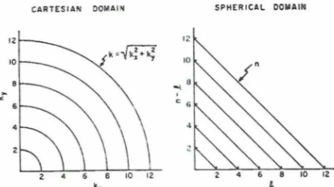
FIG. 1. Ilistrihution of the two-din~ensional scale index in terms of the two one-dimensional indices for both Cartesian and spheri- cal domains.

of waves 6-10. The observational data analyses of Wiin-Nielsen (1967) and Julian et ol. (1970) tend to substantiate a -3 energy distribution in the planetary

wave distribution.

Despite these apparently favorable observations, they are based on a one-dimensional analysis and are therefore not comparable to the expectations from two-dimensional theory; consequently, they also cannot provide a satisfactory closure condition. We must find a two-dimensional representation for the atnlosphere which yields observations corresponding to two-dimen- sional turbulence theory. Such a representation has been used by Lilly (1969) to calculate the energy distribution vs two-dimensional scale in a simple tur- bulence model with remarkable success, i.e., he calcu- lated the anticipated -3 slope. The geometry utilized by Lilly in his model is unfortunately inapplicable to the largest atmospheric scales because of the earth's curvature.

I t is the purpose of this study to present a two- dimensional scale representation applicable to varia- bles in atnlospheric surfaces (pressure or geopotential) and to describe observed energy distributions in terms of this scale. The appropriateness of the scale repre- sentation will be assessed, the region of two-dimen- sionality with regard to this scale will be established, and the -3 distribution of energy in tenns of the scale index will be highlighted. Based on the successful comparison of observed energy distributions with two- dimensional turbulence theory in terms of our pro- posed two-dimensional scale representation, that repre- sentation should lead to a suitable parameterization of shorter scales with known statistics and thereby ad- vance our understanding of the predic~dbility question.

2. An appropriate two-dimensional index

To establish an index which characterizes scales in a two-dimensional surface and which will permit an esyansion of variables in those scales, let us consider

a two-dimensional differential operator as it operates on a nornlalized function. Such an operator, say the Lnplacian (V), would by simple scale r~nalysis have the

where s2 is the overall area of the region and m is an index (the sought after two-dimensional indes) repre- senting the number of subregions (As)2 in the total domain ; i.e., (AsI2 = ( ~ / r n ) ~ .

Let us now apply this operator to a rectangular region described in a Cartesian representation wherein the function to be operated on is periodic in both dimensions. The characteristic functions with these properties are clearly given as

where

k=

k,i+k,j and r is the radius vector in the surface. By application of the Laplace operator

V f =

-k2f, where k2=kt+k,2,

and we see from m"k2s2 that the appropriate two- tlimensional indes for this domain is kZ. Indeed this is the indes which was used by Lilly (1969) in his nu- merical simulation of two-dimensional turbulence. The distribution of k2 as it depends on k , and k, is depicted graphically on the left-hand side of Fig. 1. Note that k, and k, represent one-dimensional indices of scale in the x and y directions, respectively.

For problems dealing with representation in a spherical surface (obviously applicable to the earth's atmosphere), the appropriate characteristic functions are the solid spherical harmonics

Y a (X,p) = exp (.1'JaA)Y a

(PI,

(1)

where a=na+ila is a complex wdve vector describing the two one-dimensional scales; i.e., la represents the planetary (longitudinal) scale index and nu-la the ordinal (latitudinal) index, defining the number of zeros between the poles. The longitude is represented by A, p describes the sine of latitude, and the associated Legendre polynomials (Pa) are polynomials in p of

order n,. Application of the Laplace operator to these functions leads to the well-known characteristic equation

The appropriate two-dimensional scale index is here seen to be n i ' na (nu+ l)s2, which depends not only on 12, alone, but is linearly proportional to n, for

indices not too close to unity. I t is this index then, the order of the Legendre polynomial, which we wish to explore as a possible alternative scale index for two- dimensional representation in a spherical surface. BY

suggesting our scale indes as an alternative, we imply that atmospheric variables have traditionally been de- scribed by the one-dimensional indes 2, alone and hemispheric averages have been evtracted by integra- tion over latitude of the variables as a function of l, and p. This procedure may be observed in the analj'ses

of Saltzlnltn : Julian et (11. ( The distrib one-dimensio~ rally on the larity of disi index of the given value Cartesian an fro111 Fig. 1. for each valuc of d l anlplit~ of constant i~ discuss the k dttail subseq fiied k in th m:ty not he R'e therefort structures for t) peprojectic be displayed how the cell tude (I,) and cell configura

is an repre- total ngular herein both these in the e two- this is iis nu-

:.

'The :pitted te that ~f scale in a earth's nctions scribing nts the -1, the ber of ,esented jociated in p of o these c4uation is here 3t only ) I . for hen, the wish to for two- 'ace.

H!'

;e imply been de- ,ne and integta- ion oi 1,

L;rc. 2. Ex3nipli of'ditkrent cell'corl!i~urntiu~ls all liaving the s m l e two-cliniensional in-

~ l c s , in this cast: n = 5 . The cells are defined I)>- thcir nodal lines and ;%re presented on a

>Iollweide-type projection.

of $;i.ltzn~;tn and Fleisher il!)6L), Uiiin-Nielse~l (1967 ),

Juli;tn et (11. (1970) and others.

'I'lie distribution of the indes 1 1 , in terms of the two

one-tliniensionaI indices l,,, 12,~-1, is described graphi- call! on the right-hand side of Fig. 1. Xote the simi- lari~ >. of dist.rib11 t ion be tx7ecrl this indes :uid the

L'

indcs of the Cartesian plane. 'I'he cells included in a givt n value of the two-din1ension;~l indcs in both Cartt.si:tn and spherical domains :~lso may be seen iron] Fig. 1. The total :tmplitude of a given variable for ~,;i.ch value of ;in indc:s would require t.he sunmlntion

of 2.11 a.mplitudes a t allowed intersections along n, curve

of coiistnnt indes value (k or 11,)---see Fig. 1. Wc shall clisci!ss the kinetic energy as such LL v:triable in nlore

dct:!.ii sut)sequentl\;. Although the structnre of cells for hse(l l,, in the Cartesian domain is well known, such

ma! not be the case for cells in :L spherical surf;tcc. lye therefore present. its ;in es;~mple the allowed cell struc.ti.~res for n,,=5 in Pig. 2.

By

use of the hlollweide-

Lypc. projection (Steers, 15)65), all 360" of longitude may be clihpbyed. It should he evident from this esamplt: how ihe cell structure depends upon the zeros in longi- tu(lc (:lrZj and the zeros in lalitude ( 1 2 , ~ -l,j. The limit. in

cell c.ontigurations is based on the condition for Legendre

polynomials that n ,

2

l,,. Finally, with regard t o the conventional representation in tcrms of I,, alone, 0111)

{he structure for 1=5 in Fig. 2 would come under consideration, i.e., no wave structure with latitude is qcnerally consideretl.

The argument for selecting the two-dimeusio~li~l indes presented ;tbove is based esscutially on dimensional 'tnallsis. I t is of some interest to note, however, that the wave components of a giver1 scale (e.g., Fig. 2 ) will

not inter:~ct non1ine;trly with one itnother in a two- dimensionCt1 turbulent Bow, thus sugg,rc.stin,g thcir scale independence u d supportinq our choice of inde.;. iis

'111 extension of thy results of Se:tmtan (1016) and

t'l:~tzman (1960) indicating the c\istcnc.e of an e ~ a c t solution to the nonlincnr hztrotropic vorticit! eclu;~tion subject to suitable wave truncation, the non-intcr:tction of wave components with fixed sc;tle (two dimensional) ma!^ he elucidated. C'onsiderinq the flow to be repre- sented by a streamfunction, and letting that strealn- function be sep:~rated into a zonal part ($) coniprising an arbitrary number of zonal components in an e\-- pansion of zonal harmonics ;incl a wave part (+') com- prising .In :trbitr:tr numiher of planetar) wave com- ponents of fixed ordinit1 i n d c ~ (12)-this latter choice

J O I J R N X L O F T H E - 1 T l I O S P I - I E R I C S C I E N C E S

basccl on our desire to investigate the interaction of wave conlpolients of given scale-the vorticity equa- tion may be written in a spherical surface as

where

$(p,t)

=C

ICI,,(t)Pn,(I*), 1-0

NL

$'(~JP$)

=Z

+a(!) I T a ( h , ~ ) 2u

X (c~=n+il,, 11 fixed, I,+ 0) (4)

In (3) the usual l~otatioll applies; J is the lacobian oper:ttor, f the Coriolis parameter (a linear function of p), a.nd L ;I li~leilr operator in the sulface coordinates. We have included a liileilr function for generality to allow enerqy sollrces and sinks, since the argument holds for this condition as well. T1:e first two Jacobians

in (3) and the Ja~obian of jf and $ vanish by virtue of

the fact that $ d e p e ~ ~ d s only on p [Eq. (411 and, since we have chosen only one scale 12, the Laplacian of &I

is proportional to $, i.e., V'$'= -11(12+ I)$' [Eqs. (2)

and (-I.)].

Let us first consider the time charjges of the zonal comnpoaents, $,,, (1). Multiplying (3) by P,(p) and sub- stituting the esp;~nsions from (4), we find, by utilizing the orthogonality properties of the surface harmonics, that all ternis rerllaining on the right-hand side of (3) vanish on integration over longitude. This result is also a consequence of applying the selection rules for nonlinear interacting waves presented for the spectral vorticity ehuation by Rat:r ltnd Platzman (1961). Soling, therefore, that the zonal held $ (I*) is invariant in time, let us consider the tin:e changes of the wave components ( + I ) .

We now multiply (3) by the conjugrtte of the surface harmonic for component y= IT+ IZ,, utilizing an asterisk

to denote conjugttion, and after introducing (4) inte- grate over the u~lit sphere. Expanding the Jacobians in terms of derivatives, perr'orming the differentiation with regard to h as indicated by (I), noting the time irivariance of $ and combining ternls, we find that

where

211 (IL+ I), and the anlplitude and consecjuently energy in each wave colnpocent is invariant with time. ?.his conclusion is indeed the result stated earlier that ijapc

comnpoize~zts of given scale (11) will ~zot irzteroct 1 ~ o i ~ 1 i l ~ ~ ~ ~ l ~

with oize alzotlzer irz u Pco-dimeizsionoi turbulerzt J O Z ~ .

We shall show in Section 4, moreover, that gro~vth of energy in spectral compollents due to barotropic- haroclinic instability tends to disappear sill~ultaneousl~ for all co~nponents of a given scale, when we utilize index 11 as the two-dimcnsional scale indicator.

3. Data and representation

To assess the utility of our proposed iades and a\so

to estal~lish sollle spectritl statistics of atmospheric data, we have selected to represent the wind field twice daily (0000 and 1200 GNT) for the months of January and February 1969 a t five levels (7, 5, 3, 2. j,

2 db) in terms of their spectral components. The data mere taken froin both the XhlC grid analyses arldlhe tropical (Redient) analyses, thereby providing complete hemispheric coverage. The two analyses were numeri- cally merged by a linear weighting process and were then translated to the Guri-grid (Kurihara, and Eollo- way, 1 9 6 7 ) . T h e Kuri-grid has 4705 points on the hemisphere including the pole and equator; it is etTcc- tively a latitude-longitude grid, beginning with one point a t the pole, incrementing 1.875' in latitude, increasing the nunlber of equidistantly spaced poifits on each latitude circle by four, and continuing to the equator with 192 points, thereby yielding the set of points on 49 equally spaced latitude circles.

Once the data are available on the Kuri-grid, they may be converted to a set of spectral coefficients; the method for performing this transfom~ation has been detailed by Ellsaesser (1966a) and will only be outlined here. We have analyzed both the zonal (u) and merid- ional (v) wind components. I n describing the generation of coefficients for the zonal wind, the reader should bear in mind that the meridional coefficients were derived in an identical manner. Given the data a t longitudes

A = jAh where 0 6 j< p and AX-

h i p ,

and a t latitudes

p~ where 1

<

k

<

9i to include the Southern Hemisphere,

we first expand about a latitude circle in Fourier series

(5) yielding by inversion

a$

3f _{S o t e that tve have suppressed tirlle and heicrht as}

I

D

'

cv'+iz(n+l)l-+---+g(y)

'

43 _{independent variables ;Jthough the fuJlctions do l n d d}

a/J

d~

depend upon them. The kinetic energy E2(pk) at each --

and g ( y ) depends on the linear operator

L.

The solution

T---

_-

The merging and translation of this data were programmed ant1

of (5) shows that each wave compollent y propagates carried out for us hp I)r. K. lIil~nkoda, Gl;L)T,/NOAA. I'rinceton,

a t its own constant rate with frequency

v,=l,G,/

X. J.

1:lti tude the coeff '1'11 e t rite of atmos f:~ is prt circles 01 1:~titudt: :~.pproncl The g we h a w given as In (11) which o summa ti^ (see Ells: The to t crlns of with the t lle a-ten spheric a~ fro111 the 'I'he e q u i ~ :;enerated i ion of sa i he total pansion ( lravenum r listributi~ index is p ~nspnnsion

ctruv 1:it.itucle circle ,u/; in tlie I-tv:tve I I ~ : I ~ - he c:~lc~~l:tted fro111 the sun1

. h.

tile coellicirn~s gencr;~.tetl I)!. ('8) ;1nd rcprescntcd as LI:,(,Li.;) --

4

211111*+~':';f.,*. (: 0;)

Tt mi.- be noted 1h:i.t the spccirnl e.<pnnsion recluircs

'!'llr t rnclitiona1 approucll to it sycc.t.r;~l rcprcsent-:ltion

( : ~ L L L ~ over the entire sphcsica\ SUT~;L,:C. S~IICC we h ; ~ v e

ot' atn~ospberic rncrgy ger~ernlly ends here. 'The energ>-

r _{/.': is presented :IS a fu11c.tioll of 1 for diifcrent latitude} d:lt:~ only over the 'Xorihern Hcn~ispliere, some as-

sumption on it.s dist ributiol~ over the Souther11 'ticnli-

( ircles or :t rniliicricd int e:r:it:ion c.,i /.;I over :L specified

sphere must bc made. Consistent xi t.3 ot.)scrvation, we i:itit.l~do 1)c.lt is pt:dornicd to yield :Lver;yes, some

;I ppro:Lching Iiemispht:~-ic. have nssumed tlie zon;~l j16j field 1.0 l i t syii~metric ancl

the ~~~criclional (i.) field to br antis>-nllnetric across the

T h e golcral exp;tnsion in solid harnionicr of which _{e,luntor. Call:olations of}

ml;Ll P211.gy llld llle

11.c II:LV(: SO I:Lr co~npleted o n l - tile 11jngitllc:iinal pi\.rt, is

energy in different scale groups for :tltern:~te choic-es

!!'I ven ;Ls

of s;mmztry show negligible difiere.lct:s from v a h ~ e s

;

,

-

;

, ( , +

ilo)

arrived a t bj, the above defined s~.m~:lct:ry. The cliosen

y s ) ~ n m e t r y does, howevrr, eliminnt:~ :my possiblc (.or-

relation in t.he mind componellts, eiicctivt~l?; imposing ~j.,hrrt: tbc hlnrt.ions I?;., ;o,. ~lelinril 11)- (1;). ('oniplctbg _{a con(litjon of jsorropi.}

I!IC isivcrsion, wr linrl _{For noal~.sis purposes, u-e have call LII:LI ed sc:~):~rat.el\-} ~ h c cont.1-ibut.ions from zonal : ~ n d n~cridionnl energies,

3

c

~ , . ~ ~ ~ c ~ ~ ~ ) r , c , , . j

A; L..,,i.rt) and E,jr), respectively! a.s :veil :IS the total

rlcfined bj- (12). Furtheriilore, we have cnlculnted tile

1 _{energy in each pl;Lnet:lry u:lve [see (1.3')] arid in cnch}

Z

Z

ak?l(~;ih.u~:)

J.~~'"~~\!irS.

(1 1) _{~\~o-~lilll~.~sion;11} sc;ll(. [.omponent [see (14j3. ~ . i ~ ; ~ ] l ~ ,

'3p

j i

these energies 11;ive heen est~~blished a t c:~ch :~wil;lblc I r l (1 1 j We hilvc Ill~Lcle _{t h e N ~\\-ciglll:s ,} pressure level tint1 for :1.11 tilne pcriotls. For somc _{~ ~ ~ ~ ~ ~}

\,,l,ich ort,hogollnl~,zc t j l e ~ , pol).nomials ~ on ~ i~nalyws vertic:~l averages of ~ ~ ~ dat.a l sufficed. 'I'lie i~ver- ~ ~ > i I m n l a l i o n i.e., {he)- :lrc. gol,el.;L~ecl iron] the eq,la,iOns : ~ g f i were perfor~ncd lincarlq- with regard t o pressure

i.xe Ells;~esser, 1000) by first esta1)ljshing vnl~lcs : ~ t 1 rind (3 rlb illrough quadrat.ic interpolut.ion, ;wsiilning v:Lnishing wind ;tt

I

!

:

zero and 1000 nib. Thest: vn.lues, the 1-db value de-

2

I )I P,,P;,,lP pen(dirig on those :it 2 and 2.5 d b : ~ n d I-he !)-db valtle

2;-1

depending i>n the 7- :tnd 5-(11) v:Llues, thercby scrverl

tol;L1 kinetic (,\; c r surfn,c.e is I,rivcn in :I. d011blc purpose, as they were needed for the linear

I~.rrns of tlie :~mplitudes of the c~ot.flicii.~~ts u,, and r:., ns i~nalysis to he discussed in the following sect.ion. illthough our primary concern in this papcr is with the energy distribution in terlns of 1 or n, he reader

( ~ ' + z ; ~ ) ( i . . l -7

<

( l ~ ~ , l ! . ~ , " - t 7 J ~ , ? J , ~ ) may be interested to see how thk: individual colnponcnts

(fie) distribute. We have prtparecl for this purpose

.-= E,,, ( 1 'j Fig. 3, in eflect two spcctral maps, with plancturv

wave indes on the abscissa :~.ncl zctl-0s-i11-1atit~1de indes on t.he ordinate, similar to the ~ h i l r t on the right-hand irh the energy in c:ch n-[.omponcrt Being given _{*ide of Fig 1.}

_on

_{these m:Lps we h;rve pbttecl :Llld}

1 1 1 ~ u-let-m OJI the right-h:~ild siile of ( l ? J . 7 he h m ~ i - ;in;Llvrcd the limt-na:n7,gai _sn-ricll

kinetic v)hcric :tver:i.e in t.:u-h pl:uii:ta.ry wavt- ( i ) is d c ~ c r ~ i i i n ~ ( l _{(:nergy pel-cl!nt ,,i the t(,ul ,.,nergy! for lIotll the}

from t.hc total usp;~.nsion hy 1.11' sum 01rt.r 1 1 , i.r., _{zonal and meridi:)nal winds. Of principal}

_interest,

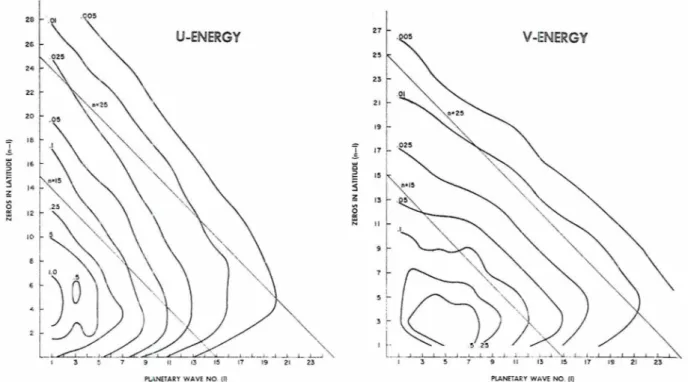
_one

obscr\res from t.hese maps t h ; ~ t for sm;~lIer .ic;lles (larger

e(l)

-C &=-C

f.:,il*,j. (1.;)

)('I k 17 index) the isopleths of const,ant energy t.encl 1-0 fo110~

lines of const:ult two-clin1ension:l1 indcs considcr:tbly '!'he criuiv;~lcnce in (13) of Icil) .with the sum oi energies more closely than the coordin;~te lints which rlufinc the :!t:nemtccl fro111 ( 0 ) i~vliich h:ls been i:riiied by _{~ ~ t i l i z a - one-dimensiolinl indices. 'This I-csult may snpport the}

1 ion of s:t~ilple d ; ~ t a ) shows the correspondencc between _{contention that the apprnpiii~te t.ru~lcai,i.,n for sp. c1;1,1}

lhe t.otal spc:c:tr;l.l exp;~nsiori (10) :i.nd the partial ex- integrntions should be triangular rather than rhanl- ~':msion ( 7 ) \ihcn only ihe (.list ribution with p1nnd:vy boidal (see Ellsacsscr! l966hj, especi:llly if one :lccrptr \ \ a v e n u ~ i ~ h e r (:L one-dimensional indes) is desired. The the 17 index as t.he approprintc two-dimensional indes

(listributioo of energy in t e r ~ u s of :L t.w-dioiensior;al _{in the spherical domain. Nevertllcless, a o,mpilrison oi}

l!lder is possililc only by i~rilixiing the i:oniplete spect r.11 Fig. 3 with :L similar figure doc]-ibing ;L recint spedrol

J(')T: R S - 4 1 - O F T H E , 1 T M O S P H E I I I C S C I E N C E S

U-ENERGY V-ENERGY

P U N E T A P Y W A V E NO (I) PIANETARY W A V E NO. (I)

FIG. 3. Average kinctic rnerg!. (holh in height and time) as a percent of total in each two-dimensional wave component, n=n+il, plotted and analyzed ns a spectral map.

Alyea, 1971, Fig. 9) shows re~narkable correspondence [and even for longer waves according to Julian e l a l .

and suggests that with adequate spectral resolution even (1970)], one is left with few waves to analyze for rhomboidal truncation will yield successful integrations. spectral statistics. Nevertheless both Julian et al.

(1c)fO) and Wiin-Nielsen (1967) find that their data

4. Linear analysis show a logarithmic decrease of kinetic energy with

If we have selected a reasonable two-dimensional incles, as argued in Section 2, we I-nay hope to find some meaningful statistical distribution in our analyzed energy data as a funct.ion of that indes. A correspon-

dence of distribution in our data with the two-dimen- sioilal t,urbulence theory as predicted by Kraichnan (1967) would necessitate an investigation of the data distribution in the spectral region beyond the scale of forcing. Since we may relate the spectral domain of baroclinic instability with the region of forcing result- ing from energy transformation, we must establish the baroclillically unstable wave region in terms of our two-dimensional indes. If there exists a cutoff indes value beyond which no instability exists, we might consider the spectral region beyond that point as euhibiting a two-dimensional turbulent structure Dre-

_-

dominantly driven by nonlinear niornentunl exchange, and with its energy source in region of baroclinic instability.

In terms of the one-dimensional planetary wave intles, most linear baroclinic stat~ility studies (Charney, 1947; Eady, 1949; Phillips, 1954; etc.) and the more recent barotropic-baroclinic stabi1it~- studies (Brown, 1969; Simons, 1970) indicate that the region of n~asi- mum instabilitv is between waves 6-10. Since current data accuracy deteriorates seriously for waves 1> 18

planetary wavenumber with a slope near -3.

To est~blish the corresponding longwave cutoff to instability (barotropic-baroclinic) in terms of our two- dimensional indes, we have solved the linearized po- tential vorticity eciuation in five atn~ospheric pressure levels (1, 3, 5, 7, 9 db) with both the vertical and latitudinal zonal tlistributions specified for each time period of available data as the zero-order state. This equation was solved in the spectral donlain and each wave component was independently superposed on the ground state and its growth rate, if existent, was calculated. The model and its program were taken from Simons (1970) and will be outlined only briefly below; for details, the reader is referred to Simon's report.

The potential vorticity equation studied has the form (also discussed t)y Phillips, 1063)

where the usual notation obt:~ins; i t . , $=$(X,p,p,t)

represents the stream field, j~ is a mean value of the

Coril bilit; chosc (196 horiz d e b (15) diff el linea zond wave wheE vectc ject strea

ft-al. .e for f1 al. data with

,IT

to two- 1 po- 'SSII re I and time 'This each 11 the WlLS i aken rief y 11on7s J,/'lGj f the

FIG. 1. Zonal wind profiles as a function of latitude and height (numhers on curves denote drcihar levels)

for two observation times and for two averaxed periods.

Coriolis parameter, u = u ( p ) is a standard static stn-

I~ility variable depending only on pressure with values

(hosen for average winter conditions given by Gates

r

1!)61), and pressure coordinates are utilized. The horizontal coordinates are latitude and longitude.

cic$ined symbolically in Section 2, and as stated above, (1.5) is evaluated at five pressure levels with finite

(liti'erencing used in place of pressure derivatives. The

liliearization hypothesis is imposed by considering the

zonal field constant in time and introducing only one

:\:~ve component then, we have for the stream field,

of the stream equation

at :~11 k latitudes of the Kuri-grit1 and the five pressure levels considered-note here why it was necessary to interpolate values at 1 and 9 clb from the given d:~t:~. The zonal espnnsion coefficients were then complited by the inversion method discussed in Section 3 from

wl~ere +o is the zonal field and a represents any wave for 1 ,( nz ,( 8, thus yielding eight coeEcients for e:~ch w4ctor in the range, 1

<

1,

<

16 and l,<n,

<

la+ 15, sub- pressure level. The wave coefficients

L

( p , / )

may also

j t t c t to the constraint that n,+la be odd. The zonal be evaluated a t each of the pressure surfaces, thus

J O U R Y A I , O F T H E A T M O S P H E R I C S C I E N C E S 4 row th 12002 18 J A N 1969 STABLE STABLE I o baroc ;L re:tsor range i r growth f 1 1 ~ app alluded

PLAN€lARY WAVE NO. (I) 1-L

-

--I -Id-L

3 s 7 9 +--iP-,k---

PLANETARY WAVE N O (I) AVERAGE FOR JAN. + RB. 1969

21 Wc h Jlllian 6 spheric the vici in midd limit ay the resi to thre x5-ould

t

the clua we do I two-din are ider

AVERAGE FOR JAN 1969

;I

STABLE 5

qo0

p

"1

2

9r

r

Wq-l

O 0

'

'!

L . . l . . i - - L l - L L - 1 - 1 I 1 . L - A - l l t I 3 S 7 9 1 1 1 3 U

PLANETARY WAVE LIO Ill

PLANETARY WAVE N O Ill

Let L planeta the rem of inde: is corn1 shorter in latit index n is that shorter been aj the poi The tribute may be Fig. 1. waves scale n which

.

This nl total ti ponellt! no con- require accept: tabulat (also c shows 1 acceptc ponent

Stability showing growth rates (e-folding time in inverse

distributions described in clays) for Fig. 4. wave componcn t s interacting with thc zonal

pressure surfaces :ire listed as of the available data sets as well as for time avenged data.

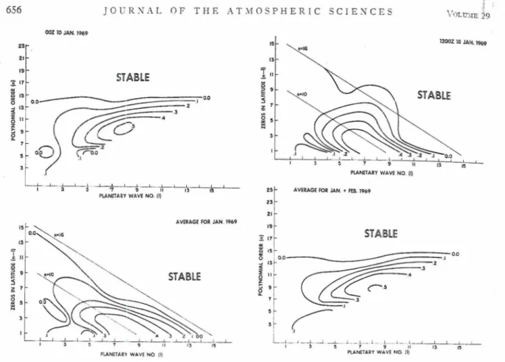
Fig. 4 describes the zonal configur;~tion for 0000 GhiT 10 January 1969, 1200 GRIT 18 January 1969, averaged data for January 1969, and a\-eraged data for January and February 1969, with the integers on the curves denoting decibar levels. VC'e have chosen the two daily profiles because of their pronounced differ- ence, one representing a single zonal jet, the other a double jet. The loss of the double jet a t 100 mb on 18

January is caused by the interpolation from the 250- and 200-mb levels. The corresponding growth rates associated with these distributions are shown in Fig.

5 , which represents the diagrams prepared from the

stability analysis discussed above. 'The positions of the diagranls in Figs. 4 and 3 correspond in time; thus, one can readily assess the impact of zonal distribution on

st ability.

The regions marked stable show no wave growth and indicate that all waves for rz> 16 are effectively un- involved in the baroclinic energy conversion process. The nlasinlum growth rates (units of inverse e-folding time in days) appear for planetary waves 1= 7-9 in agreement with the one-dimensional theory. However, these growth rates apply principally to the lowest modes (largest scale) in latitude. Indeed, the tlecay of Substituting (19) and (18) into (15) in their appropriate

series espansion, performing the necessary derivatives, and eliminating tht: horizontal space dependence by using the orthogonality properties of the Legendre polynomials (this process also involves the dis-allowance of self-interaction by the .wave components), one arrives a t the linear differential equation in time for the @-wave stream coefficient,

The (5x5) matris

A,

depends both on the static stability distribution ant1 the zonal stream coei5cients

& , - l ( p j ) for all allowed m and j, which incorporate

the vertical and horizont:il structure of the zonal field. The roots of

A,

specify the stability of the a wave and its growth rate. 'The largest imaginary component is the11 plotted on an (2, 1 2 - I ) or ( I , n) diagram -both

maps are used to familiarize the reader with these coordinates-and the calculation is perfomled for each wave coniponent within the allowed range specified above; the plotted rnaps are then analyzed in terms of these growth rates. The process is repeated for each

IAN. 1969

::i!i\:;l.h r:tlc ~r;it.ll incics is of w.ii11 a nitture ;is 1.0 yicltl i:.~:~~lc:ths of zcro growtl~ nhic.11 (.orrespond very closely

?i i! h isopleths of c-onstr~n t two-diii~ensiond scalc 11

, , . . I ,:pt for soli~e del-ifit ion in the c:~.se of ;I double jet.

T i , I [ ) J ) ~ ; L ~ s , therefore! that :I (.11:(~if index vi~lue related

1 0 i):~.~-ocIillic processes does eaist in our data, ;uid that

;, ,.i::~.son;~ble c1.1totT inclcx V ; I . I I I ~ n1:l.y i.)e chosen in the

1-;8:~;(. / I , . $ 14-16. 'l'his result, the confluence of zero

iI1-lr~~.tl~ wit11 :L ~011stfi1lt v:r.lue of index ?I, tends to

5 ) ; l ):.t:~.nti:lte our :lrpunitn t Inr sc1cc:ting this incies : ~ s ti,,. ;~.ppropri:l,t.c: two~-dirncnsion:11 indes, ;111 nrgl:n1ent;

;~Iii~t-lcd to in Section 2.

5 . Scale limit on data accuracy

'i\,-c have J r e i ~ d y inclici~.tcd, h:~:;cd on the ;ann.lysis of jl!ii;\.ti I,/ (I/.! that the rc1i;~bilitj liniit. of current ntnlo- s~)?ic~ric d:~tn in ternis of p1anet:~ry w:lvcni~r~iber is in I I ; , > vicinity of b- 16-18, r.orresponc:ling to w:tvl-lengths

il; irlicldle lariti.ldes of 1500 Ii171. Sho111d this numerical

i i i i i i t . :~pply also to the two-diniensionitl indcs N , using

t!ig' results of the prvvious sc,c:~ion for a lower cutofi 11: i.hn:c-din~ension:~.l forcing, virtu:~,lly no scale katn

I\ OIIICI be :tvnil:ible to tcsi: for statist.ica1 eq~~ilibrium in

i l i t . l-luasi t.wo~dinicnsiona1 spectral range. Fort.uni~tcly,

r i , . (lo not believe tll~tt thtr li~llit. of resolut,ion for the 1 is, !I-rlimensioni~l indcs and the p1:~netary-scale irides ;I!.(. idl-ntic:~l~ :is we s11:tll now attenipt to show.

Let us set the liil~it to reliability of dnta in terms of j)i;inctl;try scale :tt wavenumber 18, based essentially on ~!i,: results of Julian r.1 (11.. but wiih a slight relasat.ion 01' iljdes value. On the ;~:;sumpt.ion that ci:~tn re1i:lbility

i:: ~.,o~xparable in both 1;~iitude a!ld longiiude for the :~liortcr scales, we shall i~lso set the limit of reliability i l l I:ttit.ude, represented by the one-dimension:~l scale iiillcs 71-I! i1.t 18. 'Thc inip1ic;ttion of these scale li~nits i:. that-, for b o t l ~ l:~t.it~.~ciinal :tl-it1 longitudinal waves sii1)rtt.r than w:tvenu~nl.)er 18, serious snloot-hing has 1wi:n nppliec.1 which c:onsecjuently distorts the d:~t:t t o tiit: point where iriterpretnt.ion hecomes question:~ble.

I'he number of W : L Y ~ components CY which con- Li-ihute t o ;L single two-dimension:tl sc:tle 12 is IZ+ 1, ;.ts

r.::\y be clenrly seen iroln ;i.n ( l ! i r - I ) cli;tgmni such as

I'ig. 1. Indeed, Fig. 3 gives it11 cs:~mple of the incl~ldcd

i,\ ;i.ves fur rr = 5, :i.lso descri1)ing their nodes. For any :+c :~.le 11, one 111:t.y c:~lc~ul:.tte the n u n ~ b c r of components \;i>ich iLrc in the mnge of :lllowed scitles, I, 11-16 18.

'!'!>is nunlbcr is 37-n ;LII(I I I I L I S ~ be comp~~rccl to the 1 0 1 a1 n u ~ n b c r ]I+ 1. ('1e:lrly for sC:l!c.s ri

<

18 311 c o n -

ponents are in the :~c.cept:able range, whereas if ~ r > 37, 1:o c-oniponents have acct:pt:itjle d;t~:a :tccording to the ;-'.lluirenlents set. fort11 :~bove. ?he ratio (perccnt) of .~l.(:ept:ible colnponents to t.ot.al components has been. 1;lhnlated in II'i~ble 1 for two-di~.nensional scale values !:11so denoted as ordinal index) of 18<1z< 29, and :horvs tha.t for r i r 29 only 27% of the co~nponents ;Ire

::.( (.ept:~ble. Eowcver, ~ ~ e n r l y half' or illore of the com-

i:ljnel1ts may bc nccept.able for valucs of n < 2 5 . I n

'I'.%I:I.E I . Percc~lt of wnvcs \\,it11 ;rcccplal)lc ol~servalion;~l ~ i i ~ t : ~

in r : ~ h of the nrt1in:i.l index groups for IS <?z 6 20 ~ogcther with 1Iie

Ixrcmt of accepral~lt. encrgp st 111ree prcssurr Irvels.

. -- -

_

____..I.._"

. . -

Tr~blc 1. 777 represents both 1 :ind n-I, i.c., both lniist ~;tiisfy t he conditions m

<

18.

Since data are avni1:~ble for :t two-month period, wc.

may also detrrnlint: tllr percent of data in the ncccpt- able scsle r:tnge, a value which mill undoubtedly clifTer froin the percent of :~c.cept:~hle components listed in 'I'able 1. After time-averaging the l~incstic energy in each wavy component for all ci:~t;~ itt levels 700, 500

and 200 inb, we compute and list in Table 1 the percent

of energy data in the acceptable scale range (m< 18) to the total energy, together with the standard deviation for the same range of scale values, 1 8 s r z < 29. Wc note

from the table that in cscess of 5 0 ~ o of the data is ~cccptnble fol- scales w 25 except a t 200 mh.

Based on the resulis of this section and the Inst, we propose that cr re(-sonoble sc.c;lc rnlzge for t c s / i ~ ~ g two-

flinzerisio~zo/ tz~rbulcrit e,l ergy :yor/~urzgc from r~wrcni

czh)iosplrcric flat!^ is I d < ri

<

25. In this region we mnq

anticipate hoth no b:tro~:linic energy trnnsfor~~lation and rt asonabl) ;uxurate ohsenrational datn. :Innlyses

of dnta to be presented subsequent 1: will subsiantinte

this contention.

6. Spectral distributicn

T o describe the energy in different scalc components

:I.S :L function of the scale incics, TTC havc prep:~rcd

severa.1 charts (Fig. 6 ) tvhereirl energy nmplitude is plotted against wavcr,un.iher on :L log-log scale. T h c

energy groups include hoth li!I) and

L,,

for comp;~rison [see Ecjs. (13) :u:d (14) for definitions] with E,, plotted

above E f l ) on eac.:h chart. Wa have computed the zonal

srld nieridio~ial eiic-rgies sepitratelr, defined s s U and V respectively! and presented them as well as the total e ~ ~ e r g y , IT+ V. Three levels, 7, 5 :l.rid 3 db, are repre- sented and the heavy w r v e ch:~ractc.rizes the verticd mean. The periods chosen correspond to those utilized in the linear ana.lysis presented in Section 4. Solid 1inc.s denote the -3 s1:)pe.

A ct~su:tl glance itt Fig. 6 will show that we have plotted energy in the sc:lle ra.nge 5

<

1, n < 40. Howcver, our prcvious assessment of rlafn ;Lccur:lcy cleal-ly im-

J O C I I S , I I , O F T H E A T l l O S P H E R I C S C I E N C E S

FIG. 6. Spectral distributions of zonal (Lr), meridional (1/3 and total (U+V) kinetic energy for the vertical mean and decibar levels 3, .5, 7, for the two-dimensional index (n)---.upper curves--and the planetary wave index (1)--lower curves. Sections a-d corre- snond to dates utilized in Figs. 4 and 5. Solid lines denote the -3 slope.

plies that much of the data presented, indeed that for

I> 18 and n>25, is not representative. Since these

extra data are available from our source, nr~nlely KMC, and are utilized as initial data in the NNIC numerical prediction model, we attempt to show in Fig. 6 not only atn~ospherically relevant energy tlistributions, but :dso those distributions consequent on smoothing which are utilized in nun~erical forecasting. Lest the reader misinterpret this prtsentntio~l as a criticism, this writer feels that little is known about the influence of the shortest scales in a numerical prediction model, espe- cially as a function of the time period of integration, and the availability of actual initial conditions utilized

may assist in assessing the impact which the shortest scales have on predictability in terms of their spectral distribution. Our predo~ninant interest in the shorter, non-baroclinically influenced, scales led us to neglect the longest waves, those less than wavenumber 5. All

amplitudes in this and subsequent analyses are normal- ized by the total energy and the results are presented in percent.

On comparing Figs. 6a and 6b with 6c and 6d, one is in~n~ediately impressed with the variability in energy from one wavenurnber to another, a variability which effectively disappears on time averaging. Although these fluctuations are large, the energy amplitude does

FIG. scales dimens height!: Februa for fur: tend

.

decay quent range the d sentin a t les slope hle, a. applic this ir nccur: We temat ceeds corroi per le cyclo1 Since

15.0 JIR ₄₁₁ I 15.0 10.0 AK. 10.0 5.0 5.0 15.0 15.0 6.9 1 . 1 2 . 1 6.8 1.8 1 . 1 6.0 FIG. 7. Tinic dcpcndencc of wave cncrgy as n percent of total in 1.0 1.0

.;cnlcs with indices 4, i. 15 \i:~-.c, respectively), for both one- .s 2 . 0

~iimcnsionnl (1) and t~vo-dirnensiond ( 1 2 ) indices for all ohsc.rvec1

1.

. ) c : ~ ~ h t s . and the vertical meiin. Timc runs from 1 Jnnuarv t o 28 6.0

I'el~ruar!~, 1009, with 11ip n ~ n r k s denutinji missing data. See text 4.0

I'?r further tliscussion. 2 . 0

6.0 1 . 0 2 . 0 6.0 1 . 0 2.0

' -ntl to dcc:~!. with \~;~venuml)er, ;tnd statistics of this

~lt*c:ly u7ill be prescntcrl in (1u:lntitative form subse- [llrntly.

Moreover,

there is some indication, in the r,lnge of d a t a acceptability as previousl!. defined, that he distribution of cnergq appro:tches the line repre- cnting -3, if not for the planetar! wave distribution. ~t least for that of our two-di~lwnsiond index. 'The lope steepens sh;~rply for sc:~les shorter than accepta- l)le, :Ln indication that pcrhitps the smoothing operator ipplicd t o the data tends to reniove energy, howcver,

,his interpretation must be subjected to test with data ~ccurate in the shortest sc:tles.

We note further that the energy amplitude is sys-

cmnticnlly larger for all described waveb : ~ s one pro-

1 ceds to pressure levels closer to the ground. This result

orroborrites our more i1uLllitative observation that 11p- ))el. levels appe:lr inore zonal than lower levels and that I !.clone : ~ m p l i t ~ ~ d e s are relatively larger : ~ t the surface. jince our dxtn are r~onn;llizcd, t.11ere is no intlication

here of absolute amplitude; indeed the higher Iebels do attain larger energq :tnlplitudes, of which the longest waves of planetary scale have a disproportionate shnre. Perhaps the most interesting observation from Fig. 6 is the significnntlq- larger energy amplitude for all but the largest scales in the 91 relative to 1 i n d e ~ , implying that wave for wave, more energ>- resides in the two- dinlensional scale. Althouch wc do not propose to csplnin this f ~ t , we do note that each two-dimension;~l scale includes a number of planetary scales [see Eci.

(11)]. This effect holds true for the I, arid I' c onipo- nents of the energ). '1s well ;iq the totztl encrqq :~lthough, \vhcrcas the C and V components show nn equip;~rti- tion of energy in the two-dimensionnl sc:~les outside of

the ;tctively baroclinic region, the

L'

coniponcntb shon larger amplitudes than the C' conipoilents in thc planetary wave distributions. The 1:Ltter observ:ttion

may add another positive :~rqument for -electing ?z : ~ s the ;~ppropri;tte scale index.

J O U R N A L O F T H E A T M O S P H E R I C S C I E X C E S U T I N I EVERY I2 HRS, JAN I T H R U F E B 2 8 , 1 9 6 9 ) V U T V I I I

1

HEAR

1

I I I ' i ~ . l ~ ~ 3 0 . 0 1.4 I .jzo. 0 AVE. 7 ' '"c" - 10.0 .o 0

18.0; U TIHE I EVCRY I2 HRS, JAH 1 T H R U F t B Z B , 1959 V

I I I I - -. AVE. 1 2 . 0 " U TINE I L V E R Y I Z H R S , JAN 1 T H R U f E B 2 8 , 1969 1 V I I I I MBAR 1 I I 1 9 . 0

,

1 I 1 p . 0 U +V

U T l H E I EVCRY I2 HRS JAN I THRU FEE 2'2, 1969 ) 'f

9 . 0 / -, RBAR [ 1 1 I

'

(12.0 1 5 . 0 1 I 1 U t V I I

U TIN I [VERY I 2 HRS, JAN l IHRU FEB 2 8 , 1969 ) V U + V

( #BAR

1

1 I I s 1 I2.4 -- , 6.0 1 . 8 1 . 6

-

AVE. .9 0

-

. 3 JAN I 1 . 2 1.5 u *v HBlR .Z .B 1 . 0 .

--

AVE. .I .a .s n A w d h r a - .O a 0

.iuzn

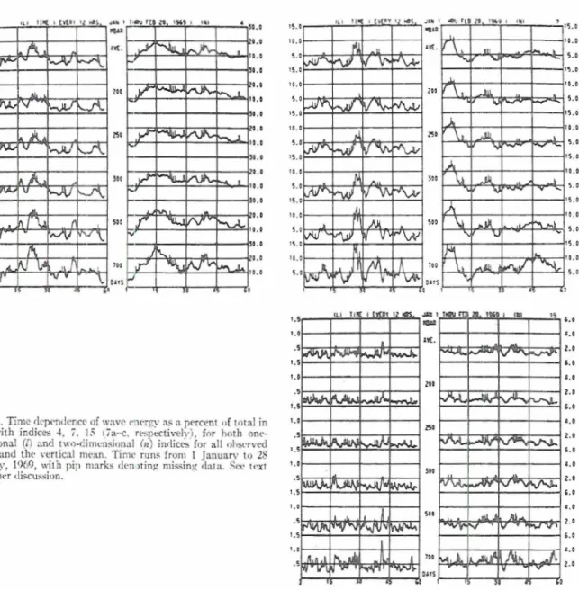
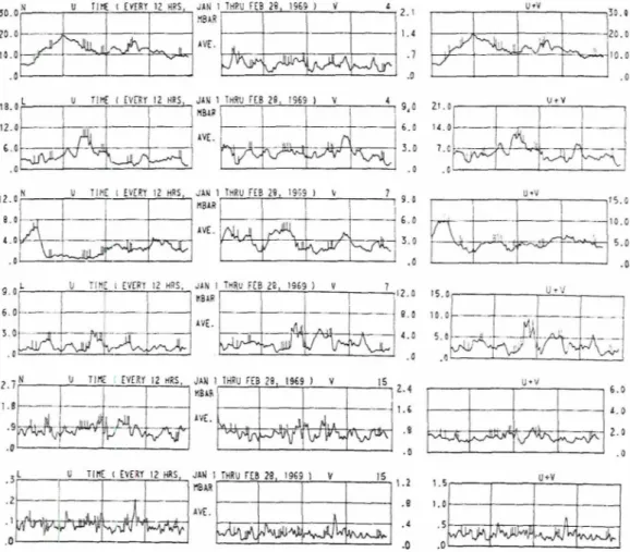
FIG. 8. Time dependence of vertical mean energy as a percent of total for waves 4, 7, 15, for both I ;uld n tlescril)ing the contributions from the zonal ( U j and meridional (V) components.

7. Time variation of energy by scale

Let us now turn our attention to the detailed varia- tion with time of the energy in the individual scale

groups, E(1) and E,,, their distribution with pressure,

and their li' and V component contributions. Since it is

in~possible t.o show all scales, we have selected three waves to represent what might be considered long, medium and short waves and given, respectively, by

indes numbers 4, 7 and 15. On Fig. 7 we present the

time variation of these three waves-Fig. 7a for wave-

number 4, 7b for 7, and 7c for 15--the left-hand chart

representing the planetary indes ( I ) and the right side

depicting the ordinal indes 07). The abscissa denotes time in days extending over the period from 1 January to 28 February 1969, and the ordinate represents corn- ponent energy as percent of total for each of the live observed levels arid the vertical mean (the uppernlost curve). Pip marks on curves of this and subsequent figures indicate times when data were unavailable.

We see from this figure that the oscillations for the I and n indices are uncorrelated in time, regardless of scale. Although such a result is perhaps obvious for the longer waves, on the assumption of isotropy in

the wave domain for the snlaller scales, one might anticipate some correlation between the one and two- dimensional representations. That the observations do not bear this correlation out indicates that for the indices chosen, the one-dimensional index (herein the

planetary wavenuniber) is ~ o t a suitable substitute for

describing the two-dimensional scale characteristics. This fact will also be apparent from the remaining presentation. As noted also on Fig. 6, the amplitude of the energy in the ordinal indes is significantly larger than that in the planetary indes for the shorter scales, an observation which is true a t all atmospheric levels.

Whereas we have seen from Fig. 6 that the relative

energy amplitude in the waves is larger a t higher pressure levels (closer to the surface), we see from

Fig. 7 that this result occurs in conjunction with larger

amplitude fiuctuations near the surface, although there is no significant change in the frequency of oscillation. One may conclude that energy eschange processes are more pronounced a t lower ievels, an effect undoubtedly related to the prosimity of the visccus boundary layer. Although the ecergy l~uctuations a t higher levels are less pronounced than near the surface, they are by no means negligible; indeed, perhaps the principal ob-

se1v of t err5 T the seen the 01114 indi, tho. ~ r i tl: relx coln the ncnl wnv oi el inde the tude scalc ener pres, of tl inch L', 1 call) ordil valu 7 an the shor

v

o amp. than the

'

Fig. sent6

F E I I D I X I \ S L ) B A E R

~ . ~ I : L P 2. T'illlc ; L V C ~ : L , ~ ~ S a i d slnnditrcl dcvintions of percent enerbqr in scale components 0 < I , vz

<

15 wit11

contributions froni the zonal (G) and meridionnl (11) parts.

_ _

.. . . ...

_

.

_ _

__

. . ...

_ _

__...

__

_

-. ... .

-. - --

-

- -- - -

-

- . .- - - --. . -. . -- .. - -

-

-- -- -.

W nvc- Planct :lrq indes Ordinal index

~ i l i n ~ b r r C I/ LT+ 1' U V I;+V

- c lv,~tion to be made Ero~u Fig. 7 is the non-constancj ,J lhe scale energy in ti111e and its significant and t I ~ I - ; L ~ ~ c variability.

The relati\-e influence of the C' and V con~ponents to

.

iic tinie variation of thc total scale energy nlny be

-(C-II froill Fig. S. Llt(lt~~se we h'1x-e already obserted r llc variation in pressure from Fi?. 7, we prcsent here ,):dy the vertical 111e.111 distributions for scales with ,11(1ices 3, 7 : ~ n d 15 and with coordinateh identical to 'hose on Fig. 7 , i t . , the 'lhscissa denotes time in d:~qs

vith 1.5 days per i n t e n d . .Is before, we note no cor- rcl;~tion between the 1 and 12 elements of the wind i onlponents. For the long w;Lv~:, with index eu,u:tl to 4, .he energy is predominantly in the zonal

(li)

compo- ?icnt, cspecially for the tw-o-diniensional indcs. 'The

.ives a i t h indices 7 :~11tl 15 show roughl~ equipartition

of cnergy between the two con~ponents for the ordinal 11des with no prono~~nccd corrtlation in tinze, although ;he conlponents ( L - ,md C? tend to have larger ampli- ude fiuctuations than the total

(C+

I.') for the shortest -(.ale. The dominance of amplitude in the V-con~ponent .nerqy for the I scales i ant1 15 is again apparent and

Lpplrs for all tinlcs (luring the ~ n a l ~ . s i s period. To assure the represrntntivcncss of the thrce scales presented in Figs. 7 # L I I ~ 8, wTe have prepared statistics

of the first fifteen sc a!es in T.lble 2. These statistics include the time olean and stxndarcl devi:ttion for the

I/', I/' :uld total wave ~omponent energies of the verti- (.ally nver:lged d'~ta. for both the planetary (I) and \)rdinal or two-tlin1nlsion:tl ( 1 6 ) ind~tes. These tabular v:~lucs do indeed Lc~rnp~lre to the ot~semations cf Figs. 7 2nd 8; tl~erc is l a y e v:lri:~l,ilit y in time for a11 sc:tles, the LT and V (-ontrib~iio~ls :Ire r0~1~171y e(4ucll for the shorter w:~ves :~ssoc.iated with the 11-in&\: whereas the

C'

~ o n t r i b ~ t i o n donlin;~tt~s for the I-index, and the eunplitude of the 11-( omponent~ is significantly larger than that of the I-components for indices

>

i.

Finally the ~ t ~ ~ t i s l i c s for t l ~ c sc:~les I O < l l < . i O are presented in

Fig. 0, with the timc (lnd veriical mean d:~ta repre- sented by the solid Lurve, f:anlced by dotted curves

defining the deviation liinits of the timc averaging. +4lthough the variability is again seen to be large, there is a tendency townrd a -3 slope in part of the scale region, a tendency which will now be csplored in greater detail.

8. Energy distribution by scale

Our observatio~ls of time niean energy distributions (Figs. 6 and 9j suggest that a power relationship may exist between the energy data and the sc:tle index in the form

E , = Amb, (21)

where m represciits the scale indes (1 for one diinen- sional and n for two dimensional), and b are con- stants, and E,, represents the energy in the m-scale

component. In (21), b clearly represents the slope on a log-log gr;tph of En, with m, and describes the ob-

6.0 JAN + Feb. 1969

1 .

ORDINAL INDEX WJ

I.'II:. 9 ,Time and vertical mean kinetic ener-!I wit11 stnntl:~rd ~ h v i a t i o n in two-dimensional sc;~les 10

<

1.1

<

30.

J O T J R N A L O F T H E A T M O S P H E R I C S C I E N C E S

L - 1 I * I , ~ - ~ - . J

17 19 21 23 25 27 29 31 2 3 25 27 29

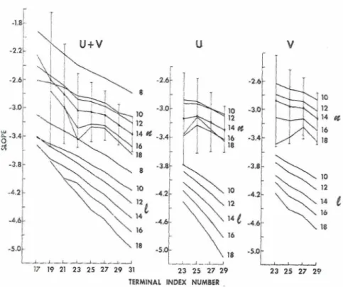
TERMlNAL INDEX NUMBER .

Fro. 10. Statistical slope of energy with scale (both I and n) for different spectral regions. Al)scissa denotes terminal index value and number following curve denotes initial index. Slopes of meridional and zonal components are also represented.

servational :malog to the energy-scale relationship anticipated from two-dimensional turbulence theory. If we define the scale region over which b is to be established from data by m,< m<ml, where mi is the

initial scale indes and m, the terminal index, and all

;V=m,--mi+l values in the allowed scale range are utilized, then by the process of least squares the data m&y be iit to the function (21) yielding b in tenns of

m, and ml, i.e.,

curves describing the I-scales are applicable, those points having values 1,=8, 10, 12 and 11= 17. I n temls

of previous investigations with this procedure, the point 1,=8, l t = 17 approaches a value b= -3 and compares favorably with the calculations of Wiin- Nielsen (1967) and Julian et ul. (1970). The remaining values for the 1-scales indicate the effect of smoothing on the initial data, and highlight the rapid reduction with scale of the zonal (U) energy relative to the meridional (I.') energy, an observation noted previously. Diverting our attention now to the slopes colnputed for the two-dimensional scale index (n), we note that for the acceptable index region previously defined,

14<n,< 25, the slope values are close to -3, and indeed do not vary significantly for variations of the terminal index in the range 23

<

nt

<

27. If one pro- ceeds into the actively baroclinic region, la,< 14, the

slope becomes less steep; if one neglects sonle baro- clinically inactive two-dimensional scales, n,> 1.2, the slope beconies more steep. These results thus tend to corroborate our earlier contention that the range

14<n<25 is the most reasonable for testing with respect to two-dimensional turbulence theory. A sys-

tematic difference between the slope of the U and V

contributions does appear, with the zonal (U) conlpo- nent energy decreasing somewhat more rapidly with scale.

Although the slope values described herein are promising by co~nparison to turbulence theory, large variability in time exists for these values (already

antic fidefi J Z i = greal of d the inclu to eI a va level some t r a y there betw large The sunln~ations in (22) go over the allowed range of

m as defined above.

The scale liniits within which we might discover distributions (slopes! coliiparable to those anticipated from turbulence theory have been defined in Section 5 .

Nevertheless, both because we have data over a wide scale range (and utilized as initial conditions for nu- nlerical integration of atn~ospheric models), we have chosen to calculate b for a wide range of values of m,

and ml. We show in Fig. 10 some values of slopes ( b )

for vertical mean time-averaged data, for the

li

and V energy components as well as the complete energy, and for both indices 1 and 11. The abscissa represents

the temlinal indes (nz,) and the numbers to the right of each curve specify the initial indices (m,).

I t is i~l~rnedialely apparent, in terms of meaningful atnlospheric data, that only s few points on all the

FIG

for tM initial*

63 ar4C

1,gc

ith

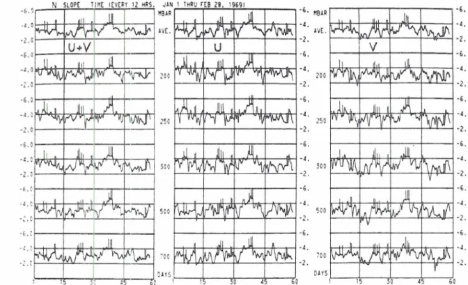
l'i,;. 11. Timc variation of slopes in the scale rcgion 14$n $25 fur all reported levels and vcrtical mean, with ct~ntrihutions

from the C. 11 components. Time period is the same as in Figs. 7 and S.

;~.niic:ip;ttcd from Fig. 6) and is expressed by the con- jidcrlcc limits (deviations) drawn for all points on the

a , = 14 curve of Fig. 10. This varittbility is described in

jisc:i.t.er detail in Fig. 11 which shows the time variation

of slope (6) for the range 14

6

11.

,<

25, including both

tlic b' and V contributions, and all reported levels

inil~iciing the vertical 2Lver:ge. It is hardly necess:lry

t o emphasize the largc anlplitude variability in time, a variahilit} which does not differ fro111 one pressure Icvcl to another, and which niay actually amplify

sonlewhat for the individual

U ,

V contrihutions. Con-

t r : ~ r y to our observation of the energy fluctuations,

t hcre appears to be some positive correlation in slope

bct.tveen the L7 and V components, principa!iy for the

1:itgcr tinle period iluctur~tions which, if significant

PI(:. 12. Vcrtical variation of statistical slo )e lti~nc avcragcd)

for the two-dimensional index with t e r m i d value of 25 and

~nitial value at Imttorn of curve. Both cnergy components (11 and

1') are tlescril)ecl ;~ncl the clot on c:ich curve clcnote* thr vcrtic:~l

cL\cr:Lge.

enough, might allow the use of either of the contribu- tions as an indicator of the total fluctudtion.

Fig. 11 also sqgests a steepening of slope with

height in the :ttniosphere. T l ~ i s effect is shown more clearly in Fig. 12 where we have plotted the slope for the 12-index in the range of 1 1 , specified a t the bottom

of the curves and terminating a t I ? , = 25 (similar results

were found for lzt=23 ;tnd 27). Thc dot on thc curves

denotes the slope of the vertical mean data, all data utilized here having been averaged in time. One sees again, as in Fig. 10, the 1owt.r 1-'tlues of slopefor the

V relative to the

li

component of encrgy. The result

of primary interest sren, however, is the si~nificant increase in slopc with altitude, especially a t the 250-mh level. One is again led to the in~clprctation oi weaker wave activit) a t higher levels, hut the predominance

of the 250-mb l e ~ e l vrith vtgard to its sterp slope is as yet unesplained.

9. Conclusion

To dr:~m- an analogy between clu:~si two-dimensional

:~tmospheric How in :L _{spherical surfncc with thc theory}

of two-dimensional turbulence, tvc have presented a.

scale representation based on the expansion of atmo-

spheric variables in spherical hsm~onics. The two-

di~nensional scale index in this case is givcn by the

order of thc Lcgcnclre poly~iomials, :~nd we have shown

thtit this index is not only ;q)~ropri;ite in tcr~ils of tlin~ensional i~n:ilysis, but t h ~ t waves oi tlie same scale