Digital Motion Control Techniques
for Electrical Drives
Sanath Alahakoon
Royal Institute of Technology
Department of Electric Power Engineering
Electrical Machines and Power Electronics
Digital Motion Control Techniques
for Electrical Drives
Sanath Alahakoon
TRITA - EME - 0001
ISSN - 1404 - 8248
ISBN - 91 - 7170 - 555 – 4
Electrical Machines and Power Electronics
Department of Electric Power Engineering
Royal Institute of Technology
Stockholm 2000
Submitted to the School of Electrical Engineering and Information Technology, KTH,
in partial fulfillment of the requirements for the degree of Doctor of Technology
1
It is believed that engineers, who were mainly trained in Power Electronics have developed the area of Motion Control. Motion control area is a result of applying control theory to power electronics. Currently it is a fairly matured field, which is almost three decades old. The research on application of microprocessors for electrical drive control in 1970’s laid the foundation stone for the Motion Control area [1]. The historical development of the Motion Control field is shown in Figure 1.1.
Power Electronics
Control Theory
Task:
Driving systems using microprocessors Computer Science Motion Control Mechanical Engineering Automatic Control Engineering Initiation of Motion Control Field - 1970's Maturation of Motion Control Field
Figure 1.1: Development of the Motion Control field
Though initiated by power electronic engineers, current status of motion control is such that conventionally trained power electronic engineers will probably require following complementary courses in motion control to grasp the development in this area. Now this field is an extremely competitive one. Nowadays, power electronics and motion control can be treated as two distinct fields that emerge as the technology advances.
Power electronics is mainly the transformation of electric power. High speed (in component switching), energy efficiency, environmental friendliness are keywords in the on going researches in this area. Achieving complete control over the motion is the fundamental idea of motion control. Obviously, this incorporates multiple fields as a typical system consists of not only electrical devices, but also mechanical components etc. Thus, motion control demands more advanced control strategies with higher degree of reliability. In most of the motion control problems, the processes under consideration are electrical machines controlled by some power electronic equipment.
The aim of this thesis is to present several digital motion control techniques that could be applied in the area of electrical drives. Before going deeper into the contents of this thesis, it is useful to have a perspective on the gradual development of digital motion control area, its present situation and the future development. From the initial introduction, it is already clear by now that motion control area is a result of the union of power electronics and automatic control theory (see Figure 1.1).
The invention of thyristors can be considered as the foundation stone of the area of power electronics. This triggered the development of sophisticated commutation circuits, as the thyristor does not have turn-off capability. This is the first phase of the development of power electronic area.
Power electronic area went through an extensive expansion during the second stage of the development, when large and small fast-switching power devices and microprocessors were introduced into the market in mid 70’s. The introduction of microprocessors into the field enhanced the possibilities of incorporating a vast amount of control theory in power electronic systems.
The key feature in the third phase of the development is the high-frequency power electronic devices. Device size can be made smaller by increasing the switching frequency. The introduction of Digital Signal Processors (DSPs) in place of microprocessors was another big step forward in this phase, which can be located in the late 80’s. The three phases of the development of power electronics are shown in Figure 1.2.
1958 1975 1976 1987 1988 1991
1st phase of power electronics
2nd phase of power electronics
3rd phase of power electronics - SCR & its applications
- Fast switching devices - Microprocessors - Control theory - Energy saving - AC drives
- High frequency power electronics
Figure 1.2: Development of power electronics through three major phases
The immediate interest of this thesis is not to go deep into the motion control problems from the power electronics point of view. Instead the approach will be to contribute to the digital motion control area from the applied control theory. Thus, the past and the recent trends of automatic control will be presented in greater detail.
1.1 Automatic control - past and present
Automatic control systems can now be found everywhere in day to day life, both in industry and domestic applications. The field by now (up to the beginning of the new millennium) is about 50 years old and is today well established. The development of automatic control is closely connected to the industrial revolution. Typical examples are the inventions of new power sources and new production techniques. Newly invented power sources had to be properly controlled, while new production techniques had to be kept operating smoothly with high product quality.
The centrifugal governor is one classical example from this era of automatic control, which has become a symbol of the field. This was mainly applied in the steam power generation and is still used in some industrial applications. Some other typical application examples from the early stages of automatic control are also worth mentioning here. Industrial process control and automation that occurred in parallel to the invention of governors is one such example. The classical PID controller still widely used in the industry is a result of this. Ship steering was another application problem, which later led the way to the invention of autopilots. Autopilots in flight control were another development that took place as early as the beginning of the century. In the meantime another
breakthrough came from the telecommunication area. This was the invention of feedback power amplifier, which has better linear operation characteristics.
With this brief description it is clear that the field of automatic control developed simultaneously as a result of attempting to solve some application problems in several different areas. The information sharing in between the application areas was not so effective. This clearly reflects from the following quotation in [2].
“Routh and Hurwitz were not aware of each other’s contributions and neither knew about the fundamental work on stability by Liyapunov”
The Second World War also motivated intensive research and development of automatic control techniques in the United States and across Europe including former Soviet Union.
1.1.1 Digital control - the second wave
Space missions started in Russia with the Sputnik in 1957 and later in the United States made a break through in automatic control. It was the first time that the computers were used for control applications [2]. Thus, physical quantities such as current, voltage, pressure, temperature etc., treated in analog form before, could then be treated as numerical figures inside a computer. This brought about an extensive flow of ideas from mathematics into the field of automatic control. The scientists were also farsighted in using advanced mathematics extensively in formulating design strategies.
This brought up new concepts such as optimisation, stochastic control, identification, adaptive control, predictive control and various other control methods.
1.1.2 Current status
The field of automatic control today is a well-established technology, which has a wide range of application areas. Some of them worth mentioning are
• Generation and distribution of electricity
• Process control in industries
• Manufacturing and robotics
• Medical area
• Various means of transportation
• Structural stabilisation and control of heating, ventilation and air conditioning in buildings
• Materials
• Instruments
• Entertainment
Whatever the application area, the approach of a control engineer nowadays to the particular problem is governed by a number of disciplines established inside the automatic control field itself. They can be briefly described as follows.
(a) Systems theory
All real systems that have to be dealt within automatic control problems can be classified into one of the following system descriptions. These are, linear systems, non-linear systems, stochastic systems, discrete-time systems, time delay systems, distributed parameter systems and decentralised systems. To describe the system behaviour, measures such as stability, observability, controllability, robustness, sensitivity, system structure etc are used.
(b) Modelling and identification
Mathematical models of systems are very important in any automatic control application. If the modelling is completely based on the physics of the particular system, it is called white box modelling. Else, it can be done by conducting experiments, which is called black box modelling. Grey box modelling is the method that uses the physics and experiments in the process. With the maturity of the systems theory, a new sub-field within automatic control called system identification was born. Today it is a well-established discipline inside automatic control area.
(c) Design
For a given process, finding a suitable controller configuration that can tackle either the servo problem or the regulation problem by following a systematic approach, is called as controller design. A lot of creativity has been shown in this area by control engineers. Most of the available methods can now be found in the form of standard textbooks and are also taught at undergraduate and postgraduate levels.
(d) Learning and adaptation
Processes that are being controlled have the tendency to change their properties and thereby dynamics with ageing. Systems that learn about such changes automatically and re-tune the controllers are very handy to have in many applications that need higher reliability throughout their operating life. Learning and adaptation is the answer for such application problems from the automatic control community.
(e) Computing and simulation
Automatic control has been tightly linked to computing throughout its development. Analog computing that was used in the beginning was replaced by digital computing later. Today there are so many mathematical computation tools specially meant for control system analysis and simulation. Examples of such tools are Matlab/Simulink, Matrixx. Some computer algebra software tools such
as Maple, Mathematica etc. are also available. (f) Implementation
This again is a very important aspect in control engineering. Implementation issues form the bridge between the theory and real application. Several practical problems that may sometimes be impossible to incorporate in the theoretical study will have to be overcome at the implementation stage. These implementation aspects are rarely addressed in highly theoretical approaches to problems in automatic control area. However, such research work has a higher possibility of producing novel theoretical contributions to the field. Yet, most of the practical problems associated with the implementation of the methods are not theoretically dealt with in many cases. It is again appropriate to quote one of the great scientists in automatic control, Karl Åström from [2].
“Many important aspects on implementation are not covered in textbooks. A good implementation requires knowledge of control systems as well as certain aspects of computer science.
It is necessary that we have engineers from both fields with enough skills to bridge the gap between the disciplines. Typical issues that have to be understood are windup, real-time kernels, computational and communication delays, numerics and man machine interfaces. Implementation of control systems is far too important to be delegated to a code generator.
Lack of understanding of implementation issues is in my opinion one of the factors that has contributed most to the notorious GAP between theory and practice.”
This thesis is meant to be a contribution that emphasises control aspects all the way down to the implementation stage, starting from the basic control theory.
(g) Commissioning and operation
Right after a control system has been designed and implemented, it has to be commissioned. Several other interesting problems may occur at this stage. Treating these issues is frequently taken up in today’s control engineering forums. In fact, a new sub-area has emerged, known as fault detection and diagnosis.
Following the above brief overview of the development of the area of automatic control so far, a quick look at available standard controller design methods will be presented in the next section. 1.1.3 Brief overview of the available methods
As the automatic control area developed and especially after discrete time control systems were initiated, a steady flow of advanced mathematics poured into controller design. Thus one can find several control design approaches that have also developed as independent sub-fields within the automatic control domain. Some of them to mention are,
• Lead-lag compensation • PID control • Optimal control • Adaptive control • Robust control • Non-linear control
• Model predictive control
These areas are very well developed today so that it is relatively easy to find good quality textbooks and publications covering each control approach [3, 4, 5, 6, 7, 8, 9, 10]. It must also be mentioned here that except for the basic control methods such as lead-lag compensation and PID control, all other methods mentioned above require a digital control platform for implementation. In fact, the whole automatic control area developed initially through analog controllers. However, even for simple motion control problems, introduction of digital control can give rise greater flexibility and better performance (even though with some limitations) [11]. A detailed comparison of merits and demerits of the two technologies giving more emphasis on motion control area can be found in [12]. The present status of motion control will be discussed in the next section.
1.2 Present status of motion control
As explained earlier, motion control has emerged from two already established fields, power electronics and automatic control theory. This makes motion control a very competitive area, covering every motion system from micro-sized to macro-sized. It has to deal with different types of actuators, mainly electrical. Some of the electrical actuators are electromagnets, DC/AC servomotors, linear motors etc.
Since motion is a mechanical quantity, any motion control system has got a mechanical component in the process of interest. As an example, in robot manipulators even if an electrical motor is the
actuator, the complete system consists of several mechanical parts that are moving and the dynamics of all components in motion have to be taken into account. The recent trend in this type of applications is to consider the dynamics of the complete system as one model in the control design [1]. This has reduced the gap between the electrical and mechanical design considerations of a particular motion control system. Developments in system identification methods have also contributed in promoting this approach. This is because the use of system identification methods makes it easier to find the input output model of the complete Electro-mechanical system (i.e. electrical actuator and mechanical components). A typical modern motion control system is shown in Figure 1.3, which elaborates this combined concept graphically.
COMPUTER
DAC
ADC
Actuators Mechanisms Process
Sensors Computer Engineering Electrical Engineering Mechanical Engineering Motion Control Networking
Figure 1.3: A typical modern motion control system
However, there are two major difficulties that modern motion control faces. One is the robustness of the control algorithms against the parameter variations of the complete system. Unlike in the case of electrical actuators, there can be other mechanical parameters such as friction, damping, wind resistance etc. that might also change with time and can have an impact on the overall controller performance. Thus the degree of parameter variation is much higher in the actual motion control application. On-line parameter estimation and adaptation is one solution to this problem.
The other difficulty is how to make the control system intelligent so that it learns from its own past experience or from the experience of an expert. Auto tuning methods [13], adaptive control techniques [6], fuzzy and neural network control systems [25] have shown some positive progress towards this direction.
With this broad overview of the history and the present status of digital motion control, it is now suitable to narrow down the focus of the discussion on to the two motion control problems related to electrical drives, which is the main topic in this thesis.
1.3 Two motion control problems under consideration
As mentioned earlier, the aim of this thesis is to present several digital motion control techniques applicable to the electrical drives area, while tackling two different applications. These applications are active magnetic bearings and high-speed permanent magnet synchronous motors. Each application carries two different motion control problems. These are precision motion control, which is applied for precise eccentric rotor positioning using active magnetic bearings and sensorless
control, which is used in sensorless control of high-speed permanent magnet synchronous motors. Both control problems are demanding and are often met by control engineers in a wide range of applications.
1.3.1 Precision motion control
Typical high precision applications include multi-axis co-ordinate measuring machines and machining of optical components [14, 15, 16]. High precision systems usually suffer from mechanical resonance that limits their closed loop bandwidths. This puts very high demands on the performance of high precision servo systems. Therefore, special digital motion control algorithms are required in order to achieve expected accuracy and speed [17, 18].
However, the actuator used in high-precision motion control applications does not have to be a servomotor. Magnetic levitation is also used in some high precision applications. One example is the magnetically levitated high accuracy positioning system presented in [19]. There, the order of positioning accuracy expected is about 30 nm. Actively controlled magnetic levitation is used to achieve the expected precise motion. Similar precision motion control applications employing magnetic levitation can be found in [20] and [21]. In such motion control applications, electromagnets are used as the actuators for the mechanical system.
Magnetic levitation principle is used in electrical drives to replace the mechanical bearings of the rotor and levitate it in air during rotation. Such electromagnetic actuators are called Active Magnetic Bearings (AMB). These are based on the idea that magnetic levitation of the rotor is actively controlled in these bearings. In the first application that is considered in this thesis, such AMBs are used to move the rotor to arbitrary radial positions in the air gap. This is done to study the acoustic noise phenomena in electrical machines that originate from rotor eccentricities in a separate project. This motion control problem will be briefly explained in section 1.4.
1.3.2 Sensorless motion control
The whole concept of feedback control is based on sensing the controlled variable (or state) of the process and feeding that information back to the controller. The task of a sensor or a transducer is to accept energy from one part of the system and emit it in a different form to another part of the system. One simple example is a thermocouple that converts heat energy into electrical energy by inducing a potential difference between the two bimetallic junctions [26]. All such sensors add some noise component into the measurement and cause some degree of deterioration in the measurement. The use of sensors needs additional cabling in the system also. Better sensors always means more cost, which will add up to the overall cost of an industrial product. Thus, reducing the number of sensors used in a control system is of utmost importance and has been a promising research area in recent years.
With the introduction of computer control to this area, there has been a vast influx of mathematics into automatic control. This has enabled modelling of the processes that are controlled and estimating some states using models running in parallel to actual processes. Such estimates can always replace direct measurement from sensors and thereby eliminate some sensors from the system.
Eliminating the shaft mounted speed sensor of an electrical drive is a very important achievement in a variable speed industrial drive. Speed sensorless operation of almost all types of AC drives (Induction, Permanent magnet synchronous, DC, Brushless DC, Switched reluctance etc.) has been an interesting area of research for a long time. This has been sighted as one of the future trends in the
new millennium in [22]. The second application considered in this thesis is sensorless control of Permanent Magnet Synchronous Motors (PMSMs) for high-speed applications. This will also be briefly outlined in section 1.5.
1.4 Active magnetic bearings for precise eccentric rotor positioning
The first motion control application considered in this thesis will be very briefly outlined in this section. The basic concept of Active Magnetic Bearing (AMB) can be described with the help of the suspended globe example. The idea here is shown in Figure 1.4 and the task is to stabilise the position of the metal sphere and maintain it at a specified distance below the electromagnet by means of a position feedback control system. This concept can be extended to make Active Magnetic Bearings. The purpose of AMBs is basically to replace the mechanical bearings on the rotor shaft of an electrical machine to achieve complete levitation of the rotating body. This requires two radial bearings for the stability in the radial direction and one axial bearing for the stability in the axial direction. CONTROLLER AMPLIFIER POSITION FEEDBACK y Metal sphere Position sensor Electromagnet Set-point -+
Figure 1.4: Basic concept of AMB – “The Suspended Globe”
An accurate method of positioning the rotor in the stator bore is essential for the study of the effect of rotor eccentricity on acoustic noise in a standard electrical machine. One way of doing this is to use eccentric rings with mechanical bearings to achieve the required eccentricity [23]. Instead of using mechanical bearings with eccentric rings, AMB actuators can be employed to carry out the noise study, provided that they are capable of precisely positioning the rotor shaft at any predefined eccentric position. Such a system essentially is superior to eccentric ring system mainly because AMB is able to mechanically de-couple the rotor from the stator. When controlled digitally, AMB system can fulfil a lot of put forward demands by the acoustic noise study of electrical machines. Digital motion control techniques that can be incorporated in elevating the rotor from the resting position to the centre of the air gap, eccentric positioning of it and maintaining the eccentric position will be presented under the first motion control application.
"Sensorless control of PMSMs for high-speed applications" is the second motion control problem that will be dealt with in this thesis. Conventional PMSM drives employ a shaft-mounted encoder or a resolver to identify the rotor flux position. This maintains the synchronism that is an essential requirement in this type of drives. But on the other hand, in most applications the presence of an encoder or a resolver causes several disadvantages. They are additional cabling cost, a higher number of connections between motor and controller, noise interference and reduced robustness. These are the reasons that raise the need to develop sensorless control schemes for PMSM drive systems. M Current sensors Inverter Voltage sensors Digital control system DC-link voltage measurement
Line current measurement
Line voltage measurement
PMSM Drive Sensorless
drive system
Three power cable connections
Figure 1.5: Basic concept of sensorless control of an AC drive
Elimination of the direct rotor position and speed measurement means that one obviously has to use as much information as possible contained in supply voltages and currents of the motor in order to extract the rotor position information. This can be done by having suitable sensors fixed closer to the control and power electronics (inverter). Thus, the number of cable connections between the control hardware and the motor is reduced to a minimum of 3 (three supply lines). In fact, this can be used as a definition for sensorless operation of an AC machine. It can be given as follows.
“If complete variable speed operation of an AC drive is achieved, while keeping the three power conductors as the only galvanic connection between the motor and the control electronics, that operation can be called as sensorless operation of the particular drive.”
The concept is graphically depicted in Figure 1.5. Different sensorless control strategies for all types of AC drives have been suggested in many publications. However, less computationally heavy, parameter insensitive and more robust sensorless control algorithms are still in demand.
In the second application considered in this thesis, a sensorless control algorithm originally suggested in [24] will be further investigated and later modified to have tracking capability of speed ramps. In addition to this, most of the implementation issues regarding the commissioning of a sensorless controlled PMSM drive will be theoretically dealt with. Thus, the outcome of this work will be a complete sensorless control drive strategy. In fact, most of the concepts that are presented here on
issues such as current control, speed control, output saturation of controllers and compensation for inverter non-idealities can be considered as general for many types of variable speed AC drives.
1.6 Overview of the thesis
As mentioned before, this thesis gives its emphasis on control aspects all the way down to the implementation stage, starting from the basic control theory. The typical viewpoint one must have on this approach of the thesis is further clarified from the following quotation of Karl Åström found in [2].
“...A long experience with journals and conferences has shown that it is very difficult to get good applications papers. The engineers, who really know about the applications, do not have the time or the permission to publish. Many of those who write have only a superficial knowledge about the applications. This sends distorted signals in all directions. There are occasional efforts with special issues of journals, where really good applications papers sometimes appear. We need those badly for better education of the next generation of control engineers.”
This thesis has two parts. The first part is on the digital control of active magnetic bearings for precise eccentric rotor positioning. The second part is on sensorless control of permanent magnet synchronous motors for high-speed applications. Both these application examples can be seen as two different test platforms used to verify the digital motion control strategies presented in the thesis. Hence, the main theme of the thesis is presenting several digital motion control techniques that can be applied not only in the two application examples discussed here, but also in many other motion control applications with suitable modifications. All motion control techniques are suggested as contributing factors in achieving the demanded control objectives in each application. Due to this reason, the two application examples will be presented as separate application reports under the title “Digital Motion Control Techniques for Electrical Drives”.
The thesis will branch out after this introduction to the thesis and the application example, “Digital Control of Active Magnetic Bearings for Precise Eccentric Rotor Positioning” will be the first part. All the work done under the AMB application will be presented in this part of the thesis.
Research on “Sensorless Control of Permanent Magnet Synchronous Motors for High-Speed Applications” is the second part of the thesis. This part of the thesis will present important information on how to implement a variable speed AC drive system practically according to the specifications. A long list of practical problems in an AC drive has been studied under this work. Thus, this application example does not limit its scope merely to sensorless control and the information given can be very useful for variable speed AC drives in general.
Reference
[1] F. Harashima, “Power Electronics and Motion Control - A Future Perspective”, Proceedings of the IEEE, Vol. 82, No. 8, August 1994.
[2] K.J. Åström “Automatic Control The Hidden Technology”, Advances in Control -Highlights of ECC ‘99, Springer - Verlag London Ltd., 1999.
[3] B.C. Kuo, “Automatic Control Systems”, Seventh edition, Prentice-Hall International, Inc., Englewood Cliffs, N.J., 1995.
[4] K.J. Åström, B. Wittenmark, “Computer Controlled Systems – Theory and Design”, Second edition, Prentice-Hall International, Inc., Englewood Cliffs, N.J., 1990.
[5] G.F. Franklin, J.D. Powell, M.L. Workman, “Digital Control of Dynamical Systems”, Second Edition, Addison-Wesley Publishing Company, Inc., 1990.
[6] K.J. Åström, B. Wittenmark, “Adaptive Control”, Second Edition, Addison-Wesley Publishing Company, 1995.
[7] M. Morari, E. Zafiriou, “Robust Process Control”, Prentice-Hall International, Inc., Englewood Cliffs, N.J., 1989.
[8] A. Isidori, “Nonlinear Control Systems”, Third Edition, Springer - Verlag London Ltd., 1995.
[9] J.E. Slotine, “Applied Nonlinear Control”, Prentice-Hall International, Inc., Englewood Cliffs, N.J., 1991.
[10] F. Allgower, T.A. Badgwell, J.S. Qin, J.B. Rawlings, S.J. Wright, “Nonlinear Predictive Control and Moving Horizon Estimation - An Introductory Overview”, Advances in Control - Highlights of ECC ‘99, Springer - Verlag London Ltd., 1999.
[11] J. Pasanen, P. Jahkonen, S.J. Ovaska, O. Vainio, H. Tenhunen, “An Integrated Digital Motion Control Unit”, IEEE Transactions on Instrumentation and Measurement, Vol. 40, No. 3, June 1991, pp 654 - 657.
[12] H. Le-Huy, “Microprocessors and Digital IC’s for Motion Control”, Proceedings of the IEEE, Vol. 82, No. 8, August 1994.
[13] K.J. Åström, T. Hägglund, “Automatic Tuning of PID Controllers”, Instrument Society of America, 1988.
[14] A.M. Higginson, S. Sanders, S. Handley, C.Wallett, “Improvements in High Precision Digital Motion Control”, Proceedings of the IEEE International Workshop on Intelligent Motion Control, Istanbul, Turkey, August 1990, Vol 2, pp 571-576.
[15] A.M. Higginson, S. Handley, “The Control and Commissioning of High Precision Mechanical Systems Using Advanced Digital Motion Control Algorithms”, IEE Colloquium on Configurable Servo Control Systems, 1994, pp 1/1-1/4.
[16] A.M. Higginson, “The Practical Implementation of Advanced Digital Motion Control Algorithms to High Precision Mechanical Systems”, IEEE/RSJ International Workshop on Intelligent Robots and Systems '91, Osaka, Japan, November 1991, Vol 2, pp 917-922.
[17] H. Fujimoto, A.Kawamura, “Perfect Tracking Digital Motion Control Based on Two-Degree-of-Freedom Multirate Feedforward Control”, 5th International Workshop on Advanced Motion Control (AMC '98), Coimbra, Portugal, June/July 1998, pp 322-327. [18] L. Guo, M. Tomizuka, “High-Speed and High-Precision Motion Control with an Optimal
Hybrid Feedforward Controller”, IEEE/ASME Transactions on Mechatronics, Vol. 2, No. 2, June 1997, pp 110-122.
[19] F. Auer, H. F. Van Beek, J. M. Van Der Kooij, “A Magnetically Levitated, Six Degrees of Freedom High Accuracy Positioning System”, Proceedings of MAG’ 95, Alexandria, Virginiya, USA, August 1995, pp 176-185.
[20] F. Auer, H. F. Van Beek, B. De Veer, “XYφ Stage with Nanometer Accuracy, Using Magnetic Bearing Actuators for Positioning”, Proceedings of MAG’ 95, Alexandria, Virginiya, USA, August 1995, pp 167-175.
[21] R.C. Ritter, P.R. Werp, M.A. Lawson, J.M. Egan, M.A. Howard, R.A. Dacey, M.S. Grady, W.C. Broaddus, G.T. Gillies, “Magnetic Stereotaxis: An Application of Magnetic Control Technology to the Needs of Clinical Medicine”, Proceedings of MAG’ 95, Alexandria, Virginiya, USA, August 1995, pp 186-196.
[22] R.J. Kerkman, G.L. Skibinski, D.W.Schlegel, “AC Drives: Year 2000 (Y2K) and Beyond”, Fourteenth Annual Applied Power Electronics Conference and Exposition (APEC '99), March 1999, Vol 1, pp 28-39.
[23] K. C. Maliti, “On Modelling of Magnetic Noise in Induction Motors”, Technical Licentiate Thesis, Royal Institute of Technology, Sweden, 1997.
[24] L. Harnefors, “On Analysis, Control and Estimation of Variable-Speed Drives”, Ph.D. Thesis, Electrical Machines and Drives, Dept. of Electric Power Engineering, Royal Institute of Technology, Stockholm, Sweden, Oct. 1997.
[25] B.K. Bose, “Expert System, Fuzzy Logic, and Neural Network Applications in Power Electronics and Motion Control”, Proceedings of the IEEE, Vol. 82, No. 8, August 1994, pp 1303-1323.
[26] D. Buchla, W. McLachlan, “Applied Electronic Instrumentation and Measurement”, Macmillan Publishing Company, Third Avenue, NY, 1992.
Digital Control of Active Magnetic Bearings for
Precise Eccentric Rotor Positioning
List of Contents
Contents i
List of symbols iv
1. Introduction 1
1.1 Use of AMB as an actuator 2
1.1.1 AMB actuator for noise study – the approach of this work 2
1.2 Brief overview of this work 3
1.2.1 Layout of the report 3
2. Experimental set-up 4
2.1 Specifications of the induction motor 4
2.2 Brief description of the AMB system 5
2.2.1 Modified end shields and rotor shaft 5
2.2.2 Control electronics 6
2.3 Digital Signal Processing System 7
2.3.1 Hardware configuration of the DSP system 8 2.3.2 Software environment for the DSP system 9 2.3.3 On-line parameter tuning using COCKPITTM 10
2.3.4 On-line monitoring using TRACETM 11
3. Modeling of the components in the AMB system 13
3.1 Mathematical model of the rotor suspension system 13
3.2 Mathematical model of the hardware electronics 15
3.3 Closed loop model of the complete system 16
3.4 Preliminary validation of the mathematical model 16
3.4.1 Frequency response of the PID controller 17 3.4.2 Frequency response of the closed loop system 18
4. Design of digital controller 20
4.1 Motivation for digital control of AMB 20
4.2 Overview of the design problem 21
4.2.1 Basic criteria for controller design 21
4.3 Discretization of the analog PID 22
4.4 Hand tuning of the PID controller 24
4.4.1 Variation of the proportional gain 25
4.4.2 Variation of the derivative gain 25
4.4.3 Variation of the integral gain 26
4.5 Integrator anti-windup scheme for AMB controller 26
4.5.1 Tracking algorithm applied to AMB controller 28
4.5.2 Verification by simulation 29
4.6 Start-up method based on bumpless transfer 30
4.6.1 Suggested start-up procedure for the digital controller 31 4.6.2 Implementation of the start-up technique 31
4.7 Final controller parameters and closed loop stability 34
4.8 Simulation and Experimental results 35
4.8.1 A small step change in set-point 35
4.8.2 Performance under an impulsive disturbance 36 4.8.3 Frequency response of the closed loop system 37
5. Model Validation and improved model for AMB 40
5.1 Closed loop AMB system description 40
5.2 Experiments for Model Validation 42
5.2.1 Time domain validation - Closed Loop Step Response 42 5.2.2 Frequency domain validation - Frequency Response 42
5.3 System Identification 44
5.3.1 Identification Experiments 44
5.3.2 Closed Loop Identification Methods 45
5.3.3 Prediction Error Method 45
5.4 Identification Results and Discussion 48
5.4.1 Identified Process Model 48
5.4.2 Model Validation 48
6. Periodic disturbance cancellation 51
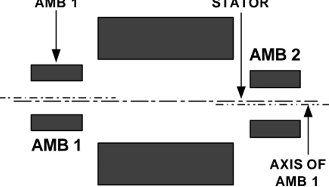
6.1 About periodic disturbances in AMB control loop 51
6.1.1 Non collocation of the geometric and gyroscopic axes of the rotor 52 6.1.2 Non collocation of the axes of AMB stators and the axis of machine stator 52
6.2 Periodic disturbance cancellation technique 53
6.2.1 Adaptive Feedforward Cancellation (AFC) 54 6.2.2 Historical development of AFC used in AMB 55
6.2.3 Discrete time AFC for the AMB 55
6.3 Tuned filter for improved adaptation 57
6.3.1 Tuned (or Notch) filter for a single frequency 57 6.3.2 Performance of Tuned Filter by simulation 58
6.4 Simulation study of the cancellation technique 58
6.4.1 Cancellation technique without noise 59 6.4.2 Performance with measurement noise and pre-filtering 60 6.4.3 Step change in set-point while APDC is active 61 6.4.4 Fluctuation of disturbing frequency while APDC is active 62
6.5 Real-time implementation of APDC technique 63
6.5.1 Real-time emulation of whirling of the rotor shaft 63 6.5.2 Cancellation of 15 Hz sinusoidal signal 64
6.5.3 Step response while rotating 66
6.5.4 Performance under frequency fluctuation 66
6.5.5 Closed loop frequency response 67
6.6 Outer digital control loop for the analog controller 68
7. Conclusions and future work 71
7.1 Main contributions of this work 71
7.2 Future work 72
Appendix A: Manufacturer data for the AMB system 76
Appendix B: Mathematical Modelling of AMB Actuator 80
List of symbols
M - total mass of the rotor (kg)
M1 - equivalent mass of rotor (kg)
J1 - equatorial mass moment of inertia (kgm2)
d - journal diameter (m)
l12 - distance between radial AMBs (m)
z1 - distance to AMB 1 from the end of the rotor (m)
z2 - distance to AMB 2 from the end of the rotor (m)
t - pole width (m)
p - number of poles of a radial AMB stator
l - length of the radial AMB stator (m)
∆α - angle of a pole arc (rad)
m - number of parallel branches in the electrical circuit
Kl - inductance factor (Hm)
δ - air gap (m)
kp - poles number factor
r - resistance/winding of radial AMB (Ω)
w - turns/winding of axial AMB
µ - permeability (H/m)
ra - inner radius of inner pole - axial bearing (m) rb - inner radius of outer pole - axial bearing (m)
Ra - outer radius of inner pole - axial bearing (m)
Rb - outer radius of outer pole - axial bearing (m) i1c - bias current of upper coil at zero eccentricity (A)
i2c - bias current of lower coil at zero eccentricity (A)
I1c - bias current of left winding of the axial bearing (A)
I3c - bias current of right winding of the axial bearing (A)
CA - power amplifier gain
Ci - current feed back gain
CT - position sensitivity (V/m)
Ca - negative stiffness due to effect of axial bearing (N/m)
Cr - negative stiffness due to radial bearing (N/m)
β21 - ratio of bias currents
1
Bearings are closely linked with all types of mechanical movement. The primary task of a bearing is to ensure smooth, low friction motion of the moving rigid body to the required degree of freedom, while withstanding the forces exerted on it from the rigid body. Mechanical engineers have developed various types of mechanical bearings to suit different applications. The word mechanical here means that the bearing of interest always has a frictional contact with the moving body and the contacting surfaces need lubrication to minimize wear and tear, friction, noise and heating due to friction. This type of mechanical bearing is disadvantageous in applications, where clean and dry environments are preferred as well as high speeds of motion is required. One example is the electrical motors used in modern textile industries, where rotational speeds of around 100,000 rpm have to be achieved. The development of electromagnetic technology, together with automatic control theory has resulted in alternative solutions such as magnetic bearings. The use of magnetic forces to overcome the forces exerted by the moving mechanical body is the prime idea of magnetic bearings. In the early stage, repulsive force between similar poles (north-north or south-south) of two carefully designed permanent magnets were used to keep the moving body away from the surface that will have to withstand the reaction forces. This concept is called passive magnetic bearings. The technology developed further and the passive magnets were replaced by electromagnets, which have varying force-current characteristics for this purpose. This enabled the engineers to have active control over the current flowing in the electromagnets used in the bearings. The ability to have active control over the performance gave these bearings the name “Active Magnetic Bearings”.
The concept of “suspended globe” that lead the way to Active Magnetic Bearing (AMB) was presented in the beginning of this thesis (see Figure 1.4 of the “Introduction to the thesis”). Since the force-current characteristic of the electromagnet has a quadratic relationship, the problem becomes a non-linear one. However, a simple controller design based on a system linearised about the required operating point can still handle this stability problem [19].
Radial AMB Radial AMB Axial AMB Effective axes of control loops Y X Rotor
Figure 1.1: A machine rotor using AMBs for complete levitation
The extension of the concept to replace the mechanical bearings of an electrical machine is graphically depicted in Figure 1.1. Each radial bearing has two axes (X, Y) for rotor movement. Thus, a control loop is required for each axis to achieve complete stability in the radial direction. This demands four independent control loops are required for the two radial bearings. Another control loop is required for the axial bearing. A complete motor drive with AMBs will therefore have five independent control loops to operate the three AMBs. Both analog and digital control strategies can be used to stabilise the rotor shaft at the centre of the air gap. The objective of this part of the thesis is to present several digital motion control
techniques that can be used to elevate the rotor and position it precisely at a required position (can also be eccentric) in the air gap.
1.1 Use of AMB as an actuator
The history of using AMBs as actuators to accomplish specific tasks other than just replacing the normal mechanical bearings has a long history. Due to feedback control, the bearing currents have direct reactions to the external forces acting on the rotor. This makes it possible to gather information on the forces acting on the rotor of a certain drive system by monitoring the bearing currents. The ability to generate forces acting on the rotor through active control is also a big advantage of using AMBs as actuators. Another important advantage is the possibility of de-coupling the rigid radial connection between the stator and the rotor, which normally exists in a conventional electrical machine with mechanical bearings. A lot of work done has been reported, where the above properties of the AMBs have been exploited to achieve particular goals. Some examples of such approaches are the analysis of the dynamic response of a rotor [1] and the use of magnetic bearings as a force generator to simulate various forces acting on a rotor under working condition [2].
The main goal for the development of the digitally controlled AMB presented in this report is to develop a high performance AMB system to be used in the study of acoustic noise in a standard induction machine. The special features mentioned above makes AMB attractive for such studies.
1.1.1 AMB actuator for noise study – the approach of this work
The study of the effect of rotor eccentricity on acoustic noise in a standard electrical machine requires an accurate method of positioning the rotor in the stator bore. One such method is to use eccentric rings with mechanical bearings to achieve the required eccentricity. This method is discussed in [3]. Instead of using mechanical bearings with eccentric rings, AMB actuators can be employed to carry out the noise study. The AMB based test rig is superior to eccentric ring system for the following reasons:
(a) AMB is able to mechanically de-couple the rotor from the stator.
Since complete levitation of the rotor is achieved, there will not be any mechanical contact between the machine housing and the rotor. This is meant by “mechanical de-coupling”. (b) AMBs offer the possibility to investigate the effect of the stiffness of the rotor
suspension system on acoustic noise (possibility of varying stiffness).
A conventional mechanical bearing also has some finite stiffness of the rotor suspension, which depends mainly on the material properties used and the construction. Hence, the stiffness can not be varied. On the contrary, stiffness of the rotor suspension system of a magnetic bearing varies, if the controller parameters are changed. This feature can be exploited to do the above study.
(c) AMBs offer the possibility to achieve static eccentricity as well as dynamic eccentricity.
Using appropriate digital motion control techniques, it is possible to force the mechanical axis of the rotor to be at a pre-defined eccentricity (Xe, Ye), while the machine is rotating.
Such an eccentricity is called as static eccentricity. It is also possible to let the rotor follow a circular eccentric path (of radius 2 2
e Y e
X + ) during rotation. This is called a dynamic
These advantages highly motivate the use of AMB as an actuator for the study of acoustic noise phenomena in standard electrical machines.
1.2 Brief overview of this work
The main objective of this work is to develop a test rig for the acoustic noise study of standard induction machines. To achieve this objective, the possibility of developing a digital signal processor based digital control system will be investigated. The objective of this approach is to provide a user-friendly environment for the noise study [48, 49, 50]. The AMB system is initially modeled using first principles with the help of manufacturer data. Later, controller designs are carried out in the simulation level, before implementing them practically. Successful implementation of the digital controller opens up several opportunities for further research. One of them is the model validation through system identification tests. Under this, the mathematically developed AMB model is validated in both time domain and frequency domain by conducting system identification experiments. Periodic disturbances occur in the position feedback signals, when the motor is rotated. An adaptive periodic disturbance cancellation method is employed to overcome this problem. This further improves the performance of the complete control strategy. Thus, the digitally controlled AMB system offers several capabilities that can lead to very important findings in the area of acoustic noise in standard induction machines.
1.2.1 Layout of the report
This part of the thesis has seven chapters.
Chapter 2 is allocated to give the details of the AMB system used in this work. It also explains the digital signal processing environment used for the controller design and implementation.
Chapter 3 describes the modeling of the components in AMB system including the controller electronics. This leads to build up a simulation model of the complete AMB control system. Chapter 4 presents the design of the digital controller and the introduction of anti wind-up and bumpless transfer techniques to overcome the problems encountered in the implementation stage.
Chapter 5 focuses on the model validation of the AMB actuator from system identification experiments.
Chapter 6 presents the periodic disturbance cancellation method used together with a description of how to improve the performance of the existing analog controller of the AMB test rig using an outer digital control loop.
Chapter 7 contains some concluding remarks with suggestions for further continuation of research in this area.
4
As mentioned in the introduction, the aim of this work is to develop a test rig for the acoustic noise study of standard induction machines. The task of the AMBs is to replace the normally used mechanical bearings in order to achieve the mechanical de-coupling between the rotor and the stator, while having controllability over the dynamic stiffness of the rotor suspension. It is therefore important to keep the overall construction of the test motor as close as possible to the construction of a standard induction machine. The solution is to use a standard induction machine with modifications to the end shields to accommodate the magnetic bearings. Modifications to the induction motor were made by an AMB manufacturer (Pskov Engineering Company in Pskov, Russia). The modified system has a complete analog control system provided by the manufacturer. However, due to several advantages that will later be explained in Chapter 4 under digital controller design, it was decided to replace the analog control system using a digital signal processor based digital controller. Necessary modifications to the hardware electronics to accommodate the digital control system were made in the laboratory. In this chapter, the important information about the induction motor and the AMBs used to replace the conventional mechanical bearings will be given. Also presented will be the details of the digital signal processing system employed.
2.1 Specifications of the induction motor
The ratings of the induction machine are as follows,Type MBT 160 L by ABB (Asea Brown Boveri Ltd.)
No. of poles 4
Rated power 15 kW Rated speed 1453 rpm Rated voltage 380/660 V Frequency 50/60 Hz
Rotor weight 35 kg (before modifications)
Air gap 0.4 mm
Air gap flux 0.93 T
The end shields of the motor are replaced by new end shields that contain magnetic bearings. Complete levitation of the rotor is achieved by means of 2 radial bearings and one axial bearing as explained in the first chapter. Figure 2.1 shows the appearance of the motor with modified end shields.
2.2 Brief description of the AMB system
Each newly designed end shield accommodates one radial bearing and one half of the axial bearing. The rotor package is left as it is in the standard machine in order to preserve the same electromagnetic characteristics between the stator and rotor. The rotor shaft is modified (elongated) in order to accommodate for the laminations of the two radial bearings and the inductive position sensors. Symmetry of load distribution is preserved during the modification of rotor shaft. This has enabled the designer to use radial AMBs with similar specifications at both ends. Detailed mechanical drawings regarding the modified rotor and the AMBs together with the specifications of the magnetic bearings provided by the manufacturer can be found in Appendix A. Only the physical arrangement of the system will be presented here with the aid of some photographs. A description about the control electronics and the modifications made to accommodate the digital signal processing system will also follow.
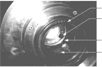
2.2.1 Modified end shields and rotor shaft
Annular stator of axial AMB
Stator of inductive position sensor of axial AMB
Stator of inductive position sensor of radial AMB Stator of radial AMB
Figure 2.2 Modified end shield
Each end shield contains the stator of one complete radial bearing. The complete stator of the axial bearing has two annular electromagnets. Each of them is fitted on the two end shields. The stators of the inductive position sensors incorporated in sensing the radial and axial motions are also fitted in the end shields. Figure 2.2 shows the inside view of an end shield.
Rotor package
Lamination for radial AMB
Non-magnetic ring for isolation
Lamination for position sensor of radial AMB
Elongated rotor shaft Figure 2.3 Modified rotor shaft
The rotor shaft is modified to accommodate the laminations of the radial AMBs and position sensors. Figure 2.3 shows the inside view of the new rotor shaft.
2.2.2 Control electronics
It is important to have an over view about the hardware electronics used to control the AMB system and the modifications made for it. Analog control system provided by the manufacturer for the AMBs is powered by ±50 V supply voltage. The control electronics have been modified so that the user can disable the analog PID controller from the system and connect the digital control system whenever required. This has enabled the user to control the same process either by analog or digital controller, depending on the requirement. Block diagram of the complete control loop to control one axis of a radial bearing or the complete axial bearing is shown in Figure 2.4. The digital controller block shown in Figure 2.4 is implemented in a DSP system. This is explained in detail in Section 2.3.
ANALOG CONTROLLER
DIGITAL
CONTROLLER THE PROCESS
Power Amplifier and AMB Actuator POSITION FEEDBACK SET-POINT ROTOR POSITION +
-Figure 2.4: Block diagram of one complete control loop
Each control loop in this system is assumed to be independent in two ways. When a single bearing is considered, a movement along X-axis of the AMB does not influence the position sensor signal of Y-axis (i.e. no cross coupling). The other assumption is any movement that take place at one AMB does not influence the position sensor signals of the other bearing. With these assumptions, it is possible to implement five independent control loops for the
control purpose of the complete AMB system (two control loops for each radial bearing and one loop for the axial bearing). Apart from these five independent analog control loops, hardware electronics required to generate the excitation carrier frequency for the inductive position sensors [18] must also be included in the system. All these are fabricated on a single circuit board and delivered as a compact box shown in Figure 2.5.
Top panel for current measurement &
reference inputs
Front panel for interfacing the DSP
system
Figure 2.5: Hardware electronics for the AMB system
The front panel that can be seen in the figure is for the connection of I/O channels of the DSP system and one can also see the switches used for the isolation of the analog controllers. On the top panel one can find the taping points to measure all bearing currents, position sensor signals and the reference inputs for position control loops.
The above brief introduction of the test rig will now be followed by a description of the digital signal processing system used for the control purpose.
2.3 Digital Signal Processing System
Selection of the Digital Signal Processing (DSP) system for the AMB application was done giving emphasis to the following important aspects:
• Sampling frequency going to be used for the AMB application
• Performance of the A/D and D/A converters
• Convenient programming platform
• Ability to perform real-time tuning of controller parameters
• On-line monitoring capability of variables in the control algorithm
• Possibility for future expansions
Typical sampling frequencies used for AMB applications fall around 10 kHz per each control loop. A/D converters without internal iterative digital filters (known as Delta-Sigma technique) were preferred in order to avoid group delays of the sampled signals due to internal filtering. Five independent control loops of the AMB system required five A/D and
D/A channels. Hardware system was selected to meet those demands. The high-level programming platform of the DSP, MatlabT M/SimulinkT M/Real-Time Interface (RTI) that will be explained in the Section 2.3.2 proved to be a very effective and user friendly software environment. The same system was later used in the research on sensorless control of permanent magnet synchronous motors with some expansions. Thus, giving emphasis on future expansion possibilities proved to be a farsighted move. Hardware environment will be explained in the following section.
2.3.1 Hardware configuration of the DSP system
The basic arrangement and the specifications of the system will be presented in this section [8,9,10]. Figure 2.6 shows the configuration diagram of the hardware set-up. The digital control system used to control the five loops in the AMB system is implemented in a DSP system, which is based on Texas Instrument TMS320C40 processor running at 50 MHz. An Analog to Digital Conversion (ADC) board with 5 independent channels and a Digital to Analog Conversion (DAC) board with 6 channels are also employed. The host PC is equipped with a Pentium 100 MHz processor and 16 MB RAM. The important specifications are given below.
(a) DS1003 DSP board with TMS320C40 50 MHz
512 KB Memory
(b) DS2001 ADC board
5 parallel 16 bit ADC channels with simultaneous sampling 5 µs conversion time
± 5 V & ± 10 V software programmable input ranges 1 MΩ input impedance DS1003 DSP Board DS2001 ADC Board 5-CH DS2102 DAC Board 6-CH PHS BUS ISA BUS HOST PC
Figure 2.6: Hardware arrangement
(c) DS2101 DAC board 6, 16 bit DAC channels
± 5 mA max. output current
2.3.2 Software environment for the DSP system
The software environment for the DSP system offered by dSPACET M together with MatlabT M and SIMULINKTM is a powerful one as it has a high level controller design, automatic code generation, real-time implementation and experimental data analysis. Software modules from three companies are associated with the overall environment. The complete set of software modules is listed below,
• TI cross C compiler Texas Instruments Inc.
• RTI40 dSPACE • TRACE40W dSPACE • COCKPIT40W dSPACE • MTRACE40 dSPACE • MLIB dSPACE • MATLAB MathWorks • SIMULINK MathWorks
• RTW (Real Time Workshop) MathWorks
The complete software-programming platform is easily explained with the aid of Figure 2.7. For programming the DSP, the user can either use C language, which is more conventional or MatlabT M/SIMULINKTM/RTI platform [11, 12]. In the second method, the controller can be built in SIMULINKTM platform by using the SIMULINKT M block models together with the additional blocks provided in RTI software by dSPACET M. This programming process becomes much faster. Since the second option was used in this case, MatlabT M/SIMULINKTM/RTI platform will be explained in detail.
Figure 2.7: Complete software environment
Once a controller is tuned for the mathematical model of the real process in the simulation level, it can directly be used to build up the real time controller block model. The dSPACET M has provided another block library called DSLIB that contains block models of all I/O devices. Therefore SIMULINKTM model for the real time controller is a combination of
appropriate I/O devices from DSLIB and the controller block extracted from simulation model built in SIMULINKTM. This SIMULINKT M model is then used to generate the C code for the DSP. This is done by a combination of software tools. They are Real Time WorkshopT M (RTW) [13], Real Time Interface (RTI) [14] and Texas Instruments C compiler [15].
2.3.3 On-line parameter tuning using COCKPITTM
There can be modeling errors between the real process and the mathematical model used for simulation, which demands fine-tuning of real time controller parameters. This is done in Windows environment using a software tool called COCKPITT M [16]. It can be operated on-line, while the real time process is being controlled by the DSP.
The dSPACE’s COCKPITT M program is an instrument panel, which provides graphical output and interactive modification of variables, for any application running on a DS1003 DSP board. It is possible to modify or display all variables represented as single-precision floating point or integer variables in the processor board’s memory. Output is performed with instruments like numeric displays, gauges, or moving bars. Variables can be modified with sliders, various buttons, or numeric input from the keyboard. COCKPITTM gives the user a pool of such controls, which can be used to define an application-specific layout. However, the COCKPITTM program is not intended for real-time data acquisition purposes like the dSPACE’s TRACET M module [17] (discussed in the next section), i.e. DSP access is not performed at fixed time steps.
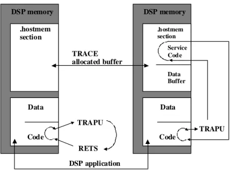
D SP m em o ry .h ostm e m se c tio n D SP a pplic ation D at a C o de D SP m em or y .hostmem section D at a C o de Inac tive C O C K P IT A c tive C O C K P IT
TR A PU
R ET S C O C K P IT alloc a ted buff er
TR A P U
Service Code
Data Buffer
Figure 2.8: Implementation of COCKPIT on the DSP
When used, COCKPITTM downloads some DSP code to the processor board, which stores data corresponding to each COCKPITT M instrument used in a table on the DSP memory. This table can be read by COCKPITTM as a block and the values of data are then assigned to the respective controls. The DSP routine also executes write operations as soon as one is requested by a COCKPITT M control. A block data can be transferred much faster to the host PC. This is faster than trying to access many randomly distributed memory locations. Other programs like TRACET M, which need accessing the DSP memory, while running parallel to
COCKPITTM are also benefited from this feature. Figure 2.8 graphically shows how the COCKPITTM mechanism that communicates with the algorithm running in the DSP.
2.3.4 On-line monitoring using TRACETM
When a digital control scheme is implemented, it is of great importance to be able to monitor the variables in the control algorithm, which is running in the DSP. For example to check whether the integrator windup is taking place, one has to have the ability to see the variation of the integrator output value of a digital PID controller. This requirement is met by another software tool called TRACET M [17]. TRACET M is capable of capturing the variation of an assigned variable over a defined period and displaying it on the host PC. If a later analysis is also required, then TRACE40 has an acquisition mode, by which one can save data as *.mat files in the host PC. Analysis can be carried out later using MatlabT M and its toolboxes.
TRACET M has the following features:
• Free-running or level-triggered mode with pre- and post-trigger
• Distinction between variables of several data types including static and dynamic data
• Variable TRACET M capture sampling rates (down sampling)
• Automatic repetitive TRACET M capture (automatic TRACET M)
• Endless TRACET M capturing without data gaps (ONLY for slow processes)
• Freely configurable order, size and position of plots
• Presentation of signals as y-t or x-y plots
The TRACET M mechanism is somewhat similar to that of COCKPITT M. TRACET M also has two different states on the DSP. First there is the inactive state, when TRACET M is not performing data acquisition. The active state is entered, when TRACET M has started data capture and the DSP is collecting the data in real-time. TRACET M uses the DSP memory to install a piece of DSP code and to store the traced data until they are transferred to the host computer. Figure 2.9 shows the mechanism.
DSP memory .hostmem section DSP application Data Code DSP memory .hostmem section Data Code
Inactive TRACE During a TRACE capture
TRAPU RETS TRACE allocated buffer TRAPU Service Code Data Buffer
The main limitation of this data acquisition method is the on-board memory size of the DSP board. Free memory space of the DSP board after the program down loading, is used to store the data temporarily. Once the acquisition is completed over the defined time interval, data is transferred to the hard disk of the PC through ISA bus. This technique imposes a limitation on the acquisition time length based on the free memory space. In other words, one has to consider the sampling period, memory occupied by the digital control algorithm and the number of variables required to be stored, when deciding the acquisition period. This is graphically shown in Figure 2.10.
On-board memory Memory occupied by the down loaded DSP algorithm
C40 Processor running the digital control algorithm
Transfering data to on-board memory of the DSP board during each program cycle
DSP Board
PC Harddisk
Transfered to PC hard disk through ISA bus & saved as *.mat file
Figure 2.10: Memory limitations for TRACE on the DSP
This is a brief overview of the DSP system used for the AMB application example in this thesis.
13
When working with real-time control systems it is essential that the design engineer does some preliminary design and simulation studies on any control strategy implemented on the real system. With such an approach one can always get rid of very basic problems that may occur such as instabilities due to wrong closed loop pole placement etc. System modelling becomes a key word in this respect. In order to build up a reliable mathematical model for the AMB actuator both the mechanical rotor suspension system and the hardware electronics have to be modelled. This chapter explains about the mathematical modelling of AMB actuator. A preliminary model validation will be made at the end of the chapter.
Generally speaking, the AMB is a Multi-Input Multi-Output (MIMO) system, where there are five inputs and five outputs. One approach to develop the mathematical model is to take the interaction of inputs on different outputs into consideration and develop a full MIMO model. In addition to the interactions among the five actuators of the AMB, there is also the presence of vibration modes of the shaft as reported in [3]. These modes are observed, even when the motor shaft is not rotating. Since the preliminary investigations with the existing analog control system shows that it is sufficient to control the five-input five-output system as 5 individual loops, instead of developing the full MIMO system, a Single Input Single Output (SISO) model for each actuator will be developed mathematically in this chapter. Developing the model for a single actuator was done based on the following basic assumptions.
1. The interactions (or coupling) from the other actuators are negligible 2. The effects of the vibration modes of the shaft are negligible.
3. The shaft is not rotating and hence the additional periodic disturbances due to whirling can be neglected.
3.1 Mathematical model of the rotor suspension system
Derivation of the mathematical model of rotor suspension system is a complex task. This is closely related with the design process of a particular AMB system. The modelling procedure must start with basic electromagnetic circuit equations, taking into account mechanical dimensions of the AMB stator and rotor. This process involves several equations based on empirical results also. The particular procedure is fully described starting from the first principles in [18]. With the basic assumptions made in the beginning of this chapter, modelling of one axis of the rotor suspension system of a radial AMB can be done considering the electromagnetic circuit shown in Figure 3.1. The procedure given in [18] was repeated to obtain the mathematical model of the rotor suspension, since it was not readily available in the information provided by the manufacturer. Appendix B describes all the key equations used in modelling and presents numerical state space models of each AMB actuator.
Due to the non-linear force-current characteristics of the electromagnets, the original model for the electromagnetic rotor suspension system becomes non-linear. This equation is linearised about the stable operating point, which is the centre of the air gap of the AMB stator that have the co-ordinate (0,0) with respect to (X, Y) axis system shown in Figure 1.1 of the introduction. In this section only the linearised state-space equation for one AMB actuator (see Figure 3.1) will be given.