Variance Adaptive Quantization and Adaptive Offset Selection in High Efficiency Video Coding

(1)

16004

Examensarbete 30 hp

Februari 2016

Variance Adaptive Quantization

and Adaptive Offset Selection

in High Efficiency Video Coding

(2)

Teknisk- naturvetenskaplig fakultet UTH-enheten Besöksadress: Ångströmlaboratoriet Lägerhyddsvägen 1 Hus 4, Plan 0 Postadress: Box 536 751 21 Uppsala Telefon: 018 – 471 30 03 Telefax: 018 – 471 30 00 Hemsida: http://www.teknat.uu.se/student

Abstract

Variance Adaptive Quantization and Adaptive

Offset Selection in High Efficiency Video Coding

Anna Abrahamsson

Video compression uses encoding to reduce the number of bits that are used for representing a video file in order to store and transmit it at a smaller size. A decoder reconstructs the received data into a representation of the original video. Video coding standards determines how the video compression should be conducted and one of the latest standards is High Efficiency Video Coding (HEVC). One technique that can be used in the encoder is variance adaptive quantization which improves the subjective quality in videos. The technique assigns lower quantization parameter values to parts of the frame with low variance to increase quality, and vice versa. Another part of the encoder is the sample adaptive offset filter, which reduces pixel errors caused by the compression. In this project, the variance adaptive quantization technique is implemented in the Ericsson research HEVC encoder c65. Its functionality is verified by subjective evaluation. It is investigated if the sample adaptive offset can exploit the adjusted quantization parameters values when reducing pixel errors to improve compression efficiency. A model for this purpose is developed and implemented in c65. Data indicates that the model can increase the error reduction in the sample adaptive offset. However, the difference in performance of the model compared to a reference encoder is not significant.

Handledare: Per Wennersten Ämnesgranskare: Marcus Björk Examinator: Elísabet Andrésdóttir ISSN: 1650-8319, UPTEC STS 16004

(3)

Sammanfattning

Video används på många olika sätt i våra vardagsliv, från att förse oss med underhållning och utbildning till att distribuera information och ge stöd för kommunikation. På grund av detta utgör video mer än hälften av internettrafiken idag, och denna andel beräknas öka ytterligare de kommande åren. Video består av en stor mängd data vilket gör det omöjligt att sända den mängd av video vi gör idag i originalstorlek. Därför används videokomprimeringstekniker som tar bort data som är överflödig från videofiler så de kan lagras och skickas i mindre storlek. Den konstant ökande videotrafiken på internet och efterfrågan av högre kvalité skapar därmed ett behov av effektivare videokomprimeringsmetoder.

Videokomprimering består av en kodare och en avkodare. För att kodaren och avkodaren ska vara kompatibla finns det videokodnings-standarder som fastställer hur video ska komprimeras, där en av de senaste standarderna är High Efficiency Video Coding/h.265 (HEVC). Målet med videokomprimering är att reducera antalet bitar som representerar videon så mycket som möjligt men samtidigt behålla god videokvalité. Den resulterande kvalitén på en video som komprimerats kan dels bedömas subjektivt, genom att människor får titta på en video och avgöra hur de upplever kvalitén, och dels objektivt, med framtagna mått som beräknar kvalitén. En viktig parameter inom videokodning som både påverkar subjektiv och objektiv kvalité är kvantiseringsparametern (QP). Den avgör hur mycket data som förloras under vad som kallas kvantiseringssteget i kodaren. Ett högt värde på QP gör att en större mängd data förloras och medför då att kvalitén på videon minskar, och vice versa. I standarden HEVC kan QP ha olika värde för olika block av en bild i videon. Därmed kan kvalitén göras bättre eller sämre för olika delar av samma bild. En videokomprimeringsteknik som utnyttjar denna möjlighet är VariansAdaptiv Kvantisering (VAQ). Den har använts i en tidigare standard, och är baserad på det faktum att människor är mer känsliga för att se fel i homogena delar av en bild, än i de som har hög textur. Tekniken tilldelar därför låga QP-värden till delar av bilden som har låg varians i pixelvärde så att kvalitén förbättras, och höga QP-värden till delar där variansen är hög. Denna teknik leder till subjektiv förbättring av kvalitén, medan objektiva mått pekar på försämring. I denna studie implementeras VAQ-tekniken i en kodare av standarden HEVC, och dess funktionalitet verifieras subjektivt.

En annan del av kodaren är Sample Adaptive Offset filtret. SAO-filtret används för att minska felet mellan pixlarnas originalvärde och det värde de har efter komprimering. SAO-filtret appliceras för varje Coding Tree Unit (CTU), vilket är det största block varje bild i en videosekvens delas in i. Genom att dela in pixlarna inom detta block i kategorier, utifrån vad deras värde är i förhållande till de intilliggande pixlarna, kan ett medelfel beräknas för varje kategori. Om medelfelet exempelvis visar att pixlarna generellt har lägre värde efter att de har komprimerats, jämfört med deras originalvärde, tilldelas alla pixlar i den kategorin med en positiv offset. Offseten är ett heltal som då adderas till varje pixels slutliga värde så att felet gentemot originalvärdet minskar.

(4)

SAO-filtret utvecklades under det antagandet att QP-värdet är detsamma i hela CTUn. Men i de flesta kodare idag används någon form av adaptiv kvantiseringsteknik vilket leder till skillnader av QP-värdet inom CTUn. Eftersom QP-värdet direkt avgör hur mycket data som förloras, påverkar det även hur stort felet blir mellan originalpixelvärdena och de slutgiltiga pixelvärdena efter komprimeringen. Därför undersöks i denna studie möjligheten att avgöra medelfelet inom kategorierna i SAO-filtret utifrån de QP-värde som pixlarna har. Med VAQ-tekniken implementerad har pixlarna inom samma CTU en stor variation på QP. Genom att ta fram en modell för medelfelet indikerar detta även vilken offset som bör väljas för att minska felet. På så vis kan pixlar inom samma kategori få olika offsets adderade, beroende på deras QP-värde, något som inte varit möjligt i SAO-filtret tidigare. En implementation av modellen och testning av olika parametervärden för den, indikerar att felet kan reduceras mer på detta sätt än då originalmetoden för SAO-filtret används. Dessa felreduceringar av pixelvärde är dock så små att det inte kan upptäckas subjektivt. Därför utförs tester med kodning av flera videosekvenser, med objektiva kvalitétsmått, för att kunna avgöra hur modellen presterar jämfört med en referenskodare. Dessa resultat visar dock endast på marginella skillnader, så ingen slutsats kan i slutändan dras om huruvida den nya SAO-modellen bidrar till en effektivare komprimeringsmetod.

(5)

Abbreviations

AVC Advanced Video Coding - A previous coding standard from JCT-VC that is the most commonly used today.

CTU Coding Tree Unit - The largest coding unit of the frame in the HEVC video coding standard.

HEVC High Efficiency Video Coding - The last coding standard developed by JCT-VC, and the standard for the Ericsson research encoder c65.

HVS Human Visual Systems - The way humans perceive information through their eyes.

JCT-VC Joint Collaborative Team on Video Coding - A group of video coding experts from the ITU-T Video Coding Experts Group (VCEG) and the ISO/IEC Moving Picture Experts Group (MPEG)

PSNR Peak Signal-to-Noise Ratio - A method to objectively measure quality in video.

QP Quantization Parameter - A parameter in the encoder which decides how much information that should be eliminated by quantization of data.

RDO Rate Distortion Optimization - Optimization of the amount of distortion against the rate required to code a video.

SAO Sample Adaptive Offset - A filter in the HEVC encoder which reduces distortion.

VAQ Variance Adaptive Quantization - A technique that adjusts the

(7)

2

1. Introduction

Video technology plays a crucial role in our everyday lives and it is used for a wide range of different reasons, from providing entertainment and education to distributing information and supporting communication [1] Accordingly, more than half of the internet traffic today consists of videos, and the amount is estimated to increase even further the coming years [2]. Video contains a lot of data, and therefore, sending the video files in original size requires too much bandwidth [3]. The convenient way to make transmissions of video files over the internet is to compress them into smaller files with digital video compression techniques. Video compression consists of an encoder and a decoder which as a pair is described as a CODEC (enCOder/DECoder). There are video coding standards in order to build compliant CODECs. One of the latest standards is called High Efficiency Video Coding/h.265 (HEVC) and was launched in 2013 [4].

The main goal of video compression is to compress or reduce the number of bits which are used to represent the video while minimizing the loss of visual quality due to the compression. With the video services being so important to us and because the demands on quality and mobility are increasing there is a constant need for advances in the video compression field [1]. Today, the new algorithms that are being employed in video compression are usually improving the efficiency by just an extra few percent.

The measurement of video quality is problematic [1]. There are objective video coding frameworks to calculate the quality of the decoded video. Although, these does not always correlate with the subjective quality perceived by humans. By implementing new algorithms in the CODEC, the measured objective quality of the decoded video might be worse even though the subjective quality is not. One important parameter in video coding is the Quantization Parameter (QP). It can be adjusted on block level to improve quality in parts of the frame that are subjectively important, and a technique that exploits this feature is called Variance Adaptive Quantization (VAQ). This technique was implemented in the open source encoder x.264, but has not been found to have been implemented in a HEVC encoder. When setting new standards the evaluation of coding algorithms are mainly objective. This has also been the case when developing the c65 encoder which is only used inside the Ericsson research department. Therefore, the VAQ technique which decreases the objective quality has not previously been considered for implementation. Other techniques that use adaptive QP which increases objective quality have, however, been implemented. Another part of a HEVC encoder is called Sample Adaptive Offset (SAO) filter and is used for signalling offsets to reduce the error between an original video and the reconstructed one.

(8)

3

1.1 Purpose

The purpose of this project is to examine the block-based QPs role in video coding and how it can be exploited to improve coding efficiency. The VAQ technique with the adaptive QP is implemented in the HEVC CODEC c65 at Ericsson and its performance is evaluated subjectively based on personal observations. An investigation of if, and how, the SAO filter can change the method of its parameter selection depending on the resulting QP values from the VAQ is done. The new way of parameter selection in the SAO filter is implemented. Performance tests of the encoder with the implemented techniques are done by coding short standard videos and evaluating them objectively against the HEVC reference software.

Question formulations

 Can the VAQ technique be implemented in an existing HEVC encoder, and how does it affect the subjective quality?

 Can the SAO filter parameters be based on the changing QP values introduced by the VAQ algorithm to improve objective performance?

1.2 Disposition

The rest of the paper is organized as follows. First, the theory behind video compression is explained. Next, the method of how the research was conducted is described. Last, the results are presented and evaluated.

(9)

4

2. Video compression

A video sequence is made up by a series of pictures, or frames, which are presented with a certain time interval [5]. A picture rate of at least 24 pictures per second is required in order to achieve the impression of motion for the human visual system (HVS). Video coding is about removing redundancy and irrelevancy in a video sequence [3]. The difference between two succeeding pictures is typically very small, which means that most of the information in the second picture is redundant and can be removed. When removing irrelevant information, it is preferable to remove details that are unnoticeable to the HVS. Sometimes a specific bitrate is required, and the bitrate describes how many kilobytes of data per second are used for representing the video [6]. Therefore, information of greater importance may be removed which causes decrease in quality. Dependent on the size of the original video and the complexity of the encoder, the time of the encoding may differ. Consequently, when encoding a video there is a trade-off between three parameters: quality, bitrate and encoding runtime.

The encoder compresses the video file into a smaller number of bits, and creates a bitstream, which contains data and information about the coding. The receiving side can decode the bitstream and reconstruct it to a representation of the original video [3]. In most video coding applications the encoding of the video is a lossy compression. This means that the reconstructed video sequence at the decoder does not completely corresponds to the original input video sequence, some data has been lost.

2.1 Video frame

A frame in a video sequence is a matrix, or a set of matrices, of samples with intensity values [5]. The samples can also be referred to as pixels. The most common way to represent colour and brightness in full colour video coding and transmission, is to use one luma and two chroma signals. The luma value is usually described by Y, and is the grey level intensity of a sample, the brightness. Cb and Cr stands for the chroma values which represent the extent to which the colour differs from grey towards blue and red [7]. With the YCbCr colour space the luma and chroma values are sent in different channels which is preferable in video coding since the HVS is more sensitive to changes in brightness than in colours. The usual YCbCr format for the latest coding standards has 4:2:0 sampling which means that for each four luma sample there are two chroma samples. This means that the resolution in the horizontal direction and vertical direction for the chroma components is half of the full luma resolution. The sample values in the YCbCr colour space are represented by 8 bit which means with a number between 0 and 255.

The number of pixels that the frames in a video consist of is defined by its resolution [8]. Higher resolution means more pixels on the screen, and leads to higher definition of the images. High definition (HD) video sequences are for example 1280 x 720 pixels

(10)

5

per frame, or 1920 x 1080 pixels per frame. A higher resolution requires more data, hence, a bigger video file.

2.2 Video coding standards

In the 1980s the need for exchange of compressed video data on national and international basis grew larger [9]. Compatible encoders and decoders were necessary, which meant that video coding standards had to be set. The video coding standard can be said to define the language that the encoder and the decoder use to communicate [10]. It should also support good compression algorithms as well as efficient implementation of the encoder and decoder. The presence of standards allows for a larger volume of information to be exchanged and the ability for manufacturers to build standard compliant CODECs. This means that video coding standards are very important to a number of major industries and is crucial for technologies such as DVD/Blu-Ray, digital television, internet video and mobile video [3].

Today, the most common standard is the Advanced Video Coding (H.264/MPEG-4/AVC) which was finalized in 2003 [7]. It has displaced previous standards and is widely used in many applications, from broadcasting of HD TV signals over satellite, camcorders and Blue-ray Discs to real-time conversational applications such as video chat and video conferencing. The AVC standard was produced by the ITU-T Video Coding Experts Group (VCEG) and the ISO/IEC Moving Picture Experts Group (MPEG) standardization organizations, which are working together as the Joint Collaborative Team on Video Coding (JCT-VC).

2.3 High Efficiency Video Coding

The JCT-VC group also produced its most recent coding standard High Efficiency Video Coding (H.265/HEVC) in 2013 [7]. The need for a new standard with coding efficiency superior to AVC arose with the increased traffic caused by applications targeting mobile devices and tablets and the desire for higher quality and resolution in videos [7]. HEVC typically compresses a video to half the size of its precursor AVC but still maintains the same video quality [11]. Moreover, HEVC focuses on two key issues: increased video resolution and increased use of parallel processing architectures [7].

2.3.1 Encoding process

The coding process of HEVC is quite complex but to simplify, it can be described by the following steps: picture partitioning, prediction, transformation, quantization, and entropy coding [7]. An overview of the encoding process can be found in Figure 1.

(11)

6

Figure 1. The HEVC Encoding process.

PictureaPartioning

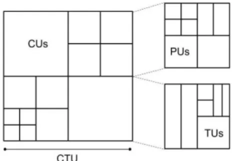
In the encoding, each picture in the video sequence gets divided into a set of non-overlapping blocks [5]. The largest blocks are called coding tree units (CTU) which can be further divided into smaller squared shaped blocks which are called coding units (CU). Each CU can be as large as their root CTU or divided into the size of 8x8. These CUs can be split into several prediction units (PU) which sizes can range from 64x64 to 4x4 pixels. HEVC also allows some asymmetric splits into non-square PUs. The CUs are also divided into transform units (TU). The size of the TUs can range from 32x32 to 4x4 pixels, and can also be non-square sized such as 4x16 or 32x8 pixels [12]. Figure 2 shows an example of a possible block structure derived from a CTU.

Figure 2. A coding tree unit (CTU) is divided into coding units (CU), which are further divided into prediction units (PU), and transform units (TU).

Prediction

The prediction model in the encoder takes an uncompressed video sequence and attempts to reduce redundancy by exploiting the similarities between the video frames,

inter-picture prediction, or within it, intra-picture prediction, by constructing PUs from

the current CU [3]. The prediction data consists of a set of model parameters, which indicates the prediction type or describes how the motion was compensated. The prediction value of each pixel is compared with the original, and the difference, the residual, gets stored. The residual is encoded and sent to the decoder which will re-create the same prediction from the prediction data and add the residual to it which will represent the current CU. The better the prediction process is, the less energy is contained in the residual.

(12)

7

Intra-xandxinter-picturexprediction

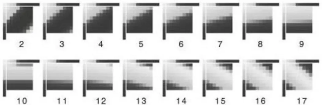
The frames in a video sequence have different names dependent on how they are predicted [3]. In I-frames only intra-picture prediction is used. This means that the frame is coded without referring to any data outside the current frame. Only samples from adjacent, previously coded blocks are used to predict the values in the current block. Since the first frame in a video sequence does not have any previous frames to refer to, it is always an I-frame. The prediction is based on one of many available modes [7], and some of the directional modes available are shown in Figure 3. The intra mode predictions are based on the previously coded pixels above and to the left of the current block. Intra-picture prediction is exclusively used in I-frames but can also be used for prediction of blocks in other types of frames when it is a better choice. Videos are usually coded with I-frames on set intervals. This allows random access, which means that if a video gets started in the middle, the video only needs to decode the few frames from the previous I-frame.

In inter-picture prediction the predictions are based on data from one or more reference pictures [13]. The encoder searches through a set of other pictures, before or after the current one, to find an area of the same size that most resembles the current block. The offset between the positions of the referenced area to the current block is called a motion vector [3], and is included in the coded data. The frames only using reference pictures from before its own position in display order are called P-frames, while frames using reference pictures from before and after are called B-frames. In Figure 4, an inter-picture prediction is being showed, where “poc” is a B-frame.

The group of pictures (GOP) structure defines in which order the I-, P- and B-frames are arranged. When encoding, the structure of the frames can also be hierarchical with different kinds of frames in different layers.

Figure 3. Examples of different intra modes in blocks of size 8. Samples from adjacent, previously coded blocks above and to the left of the current block are used for

(13)

8

Figure 4. Inter-picture prediction between blocks from different frames. Poc is a B-frame and gets predicted by previous and succeeding B-frames. [14].

Transformation

The residual data remaining after prediction are coded using block transforms [7]. A discrete cosine transform is used in order to convert the data into the transform domain [11]. Instead of storing all the residual data it can now be represented by a smaller number of transform coefficients which requires less memory, without any loss of information.

Quantization

The next step of the encoder is quantization of the transform coefficients [11]. The quantization of the coefficients is done by division with a quantization step size (Qstep) [11]. This is done to decrease and round off the values of the coefficients, and to set the coefficients with insignificant magnitudes to zero [3]. Consequently, the output consists of a sparse array of quantized coefficients, mainly containing zeros. The Qstep is decided by the QP as:

𝑄𝑠𝑡𝑒𝑝(𝑄𝑃) = (21/6 )(𝑄𝑃−4) (1) The QP values range from 0 to 51. If the QP and the Qstep is large, the range of quantized values is small and insignificant values are set to zero. Therefore the quantized data can be highly compressed during transmission [3]. However, when the quantized values are re-scaled in the decoder they become a coarse approximation to the original values. In contrast, a smaller QP leads to a better match of the re-scaled values to the original ones but at the cost of compression efficiency. Accordingly, a low QP ensures higher video quality but worse compression, and a high QP leads to worse video quality but good compression. The quantization is about removing information and it is optimised by carefully controlling the QP value so that irrelevant information can be removed instead of relevant [5]. In most encoders a defined QP value can be set as a parameter when coding a video. That value makes the starting point for the encoder to calculate the resulting QP values for the blocks and frames in the video. The resulting QP values depend on many different aspects of the video sequence being encoded. However, the size of the input QP value always has the same effect on quality and coding efficiency as mentioned above.

(14)

9

Entropyxcoding

Entropy coding is a lossless data compression scheme used at the last stage of encoding [15]. The entropy coder used in HEVC is Context-based Adaptive Binary Arithmetic Coding (CABAC). It uses certain probability measures to reduce statistical redundancy in the data. The entropy encoder produces a compressed bitstream which consists of block structure, coded prediction parameters, coded residual coefficients and header information [3]. The bitsream is sent to the receiving side which through decoding reconstructs it to a representation of the original video.

2.3.2 In loop filters

During the video encoding process, especially during the quantization step, the subjective quality may deteriorate due to the loss of data [16]. In order to compensate for this and to increase the subjective quality in the video, filters are implemented in the encoder. They are applied at the last step of the encoding, where suitable filter coefficients are determined and explicitly signaled to the decoder [16]. In HEVC, a de-blocking filter is applied, followed by the sample adaptive offset filter (SAO). The filters can also be activated separately.

De-blockingxfilter

The de-blocking filter is applied to the edges of the PUs and TUs in order to reduce the visible block structure in the frames, which can occur due to the block-based nature of the coding scheme [5]. In Figure 5, the block-structure is visible in the picture to the right, in the down right corner. The properties of the neighbouring blocks define the strength of the filtering, and the difference between the edge sample values decides if the filter should be applied or not.

SamplexAdaptivexOffsetxfilter

The purpose of the SAO filter is to reduce undesirable visible artefacts such as ringing artefacts, and the mean error between original and reconstructed samples. Where the reconstructed sample values are the ones the decoded videos samples will have. In Figure 5, ringing artefacts are noticeable next to the hat, in the picture to the right.

Figure 5. Original image to the left, and compressed image to the right showing ringing and blocking artefacts [17].

(15)

10

The SAO filter categorizes pixels of a CTU into multiple categories based on a specific classifier [18]. An offset, a positive or negative integer, is obtained for each category and is then added to each sample in the category. For example, if the reconstructed samples in a specific category seem to have smaller values than the original values, a positive offset will be applied that category, and the error will be reduced. The categorization classifier in SAO is either the band offset classification or the edge offset classification. In the band offset classification the intensity of the samples are considered [16]. The sample value range from 0 to 255 is equally distributed in 32 bands containing 8 values each. For each band, the average difference between the original and the reconstructed samples are calculated and represent the offset for that band. If the sum of all errors in a category is close to zero there is no reason to apply an offset, since a positive offset will improve the negative errors but worsen the positive errors just as much. The offset for the four most significant consecutive bands will be signalled.

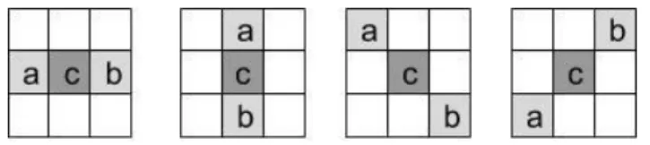
In edge offset classification, comparison between neighbouring samples is made. It uses horizontal, vertical, 135° diagonal and 45° diagonal directions to classify the samples into one out of five categories. The different directions are shown in Figure 6. The value of the current sample ‘c’ is compared to the two neighbours’ values according to the directions [18]. If, for example, both neighbours have values larger than the current sample it is placed in category 1. The classification rules for all the categories are represented in Table 1. The offset values are calculated in the same way as in band offset but category 1 and 2 are restricted to positive offset values while category 3 and 4 to negative ones, and the offset values can only be an integer between -7 and 7. The direction that gives best gain in error reduction is chosen, and the offsets for each category in that direction are signalled. The SAO filter is only used when error reduction is big enough to compensate for the cost of signalling the offsets.

Figure 6. Direction 0 to 3 for edge offset classification in SAO. Table 1. Conditions for the five edge offset categories.

Category Condition 1 c < a and c < b

2 (c < a and c == b) or (c == a and c < b)

3 (c > a and c == b) or (c == a and c > b)

4 c > a and c > b

(16)

11

2.4 Variance Adaptive Quantization

The VAQ technique was first introduced by the open source video encoder x.264 [19]. It is based on the notion that the HVS is more sensitive to distortion in a relatively homogenous area than in an area with high contrast. The technique offers significant subjective improvement in parts with a distinct texture but low variance in the pixel values. It could for example be a video with grass fields or branches of trees, see an example in Figure 7. An adaptive QP is used, which increases in value and lowers the quality for areas where there is a big difference in pixel values, whereas more homogenous areas get lower QP and higher quality. In x.264 the variance is calculated for each macroblock, which were used in AVC and has a size of 16 x 16 samples. The change of QP value for a macroblock is calculated through equation 2.

∆𝑄𝑃 = 𝐷 × (log(𝑉_{𝑏𝑙𝑜𝑐𝑘}) − log (𝑉𝑓𝑟𝑎𝑚𝑒)) (2)

Since the quantization step is exponential dependent on the QP, the use of log(variance) to change QP in this case is equivalent to using variance to change Qstep [19]. The constant D in x.264 has value 1.5 and has been decided empirically.

Figure 7. Screenshot from a video sequence [20]. The black oval shows an area where the VAQ technique gives significant improvement in subjective quality.

2.5 Rate-distortion optimization

For each block, the encoder has to choose which coding mode and prediction parameters to use [5]. The selection is made using rate distortion optimization (RDO). Given a constraint on the bitrate, R, the method tries to optimize the coding to minimize the distortion, D, through the joint cost, J, see equation 3. RDO measures the deviation from the original video and the bit cost for each possible solution. The bits are multiplied by the Lagrange multiplier, lambda (𝜆), which represents the relationship between bit cost and quality for a certain quality level. The λ can be calculated by the QP value in the current CTU as in equation 4.

(17)

12

𝐽 = 𝐷 + 𝜆𝑅 (3)

𝜆 = 0.57 × 2𝑄𝑃/3 ₍₄₎

2.6 Video compression evaluation

As previously mentioned, there is a trade-off between three parameters when encoding a video; the quality, the bitrate and the encoding runtime. These parameters are the basis on which the video coding gets evaluated. Encoding runtime represent the time it takes for a video sequence to get encoded and will not be explained any further.

2.6.1 Objective quality

The easiest way to measure the quality performance of a video compression technique is to do it objectively using algorithmic quality measures [3]. There are different ways to do this but one of the most common measure is the Peak Signal-to-Noise Ratio (PSNR) [21]. It is widely used in evaluating CODEC performance or as a comparison method between different video CODECs [22]. The PSNR measures the mean squared error between an original signal and the reconstructed signal to the available maximum amplitude of the signal [5]. Accordingly, low PSNR usually indicates low quality and high PSNR usually indicates high quality in a given image or video frame.

2.6.2 Subjective quality

It is estimated that 70% to 90% of the neurons in the human brain are dedicated to vision which indicates the importance of visual information [1]. However, typical video encoding frameworks do not always correlate with the way humans perceive visual information. Even though the mathematical distortion is minimized it does not mean that the video quality a human perceive is optimal. Therefore, [1] suggests that a better understanding of the subjective perception of visual signs and the HVS could provide significant technical advances in video compression. For example our differing sensitivity to certain types of contrast, movement and textured patterns can be considered to improve compression efficiency.

2.6.3 Bitrate

An important specification for a video is its bitrate [6], which describes how many kilobytes of data per second are used for representing the video. In video coding in general, a higher bitrate will produce a higher image quality in the video output. However, video in a newer CODEC such as H.264 will look substantially better than in older CODEC like H.263 even for a fixed bitrate. Since the main goal of video compression is to reduce the number of bits which is used to represent the video the bitrate is an important measure for evaluating the compression technique.

(18)

13

2.6.4 BD rate

Video coding is about reducing the number of bits, but maintaining good video quality. Therefore, both PSNR and bitrate has to be taken into account when evaluating the performance of an encoder. Either the PSNR value or the bitrate has to be the exact same values in order to compare two encoded videos. Since this is difficult to accomplish, the Bjøntegaard delta (BD-rate) allows an alternative comparison method of compression performance [23]. For a fixed PSNR value, the BD rate calculates the average percentage of loss or gain in bitrate between the coded videos. A negative value indicates a lower bitrate and a positive value a higher.

(19)

14

3. Method

In this project, the VAQ technique was implemented in an HEVC encoder. The main focus was to examine if the SAO filter parameters successfully could be based on the resulting QP values from the VAQ algorithm. Since the project investigated a new idea not yet explored, an iterative working method was used. Data was extracted and code was designed, implemented and tested in repeated cycles. This section describes how the work was conducted. It describes which assumptions and delimitations were made, and the implementations and calculations that were done.

3.1 Implementation of Variance Adaptive Quantization

The first step was to implement the VAQ technique in c65. The HEVC CODEC resembles the AVC CODEC in many ways, but one of the benefits of HEVC is the introduction of larger block structures with flexible sub partitioning mechanisms [12]. The VAQ algorithm is based on block sizes, and changes the QP value for TUs, and is therefore likely to function in a HEVC encoder as well. To implement VAQ in c65, a study of x.264 was done. The change of QP values in x.264 is determined by equation 2, and the variance V for each block is calculated as

𝑉(𝑥) = 1 𝑛∑(𝑥𝑖− 𝑥𝑖) 2 𝑛 𝑖=1 (5)

where 𝑥_𝑖 is the pixel value for the i:th pixel, 𝑥_𝑖 is the mean value of all the pixels in the block, and 𝑛 is the total number of pixels in the block. Since the HVS is more sensitive to the change in brightness than in color, the luma value is the most important pixel value and the only value that is used for the implementations in this project. The VAQ was implemented in c65 based on Equation 2 and 5, where D in Equation 2 was set to 1.5 the same value as in x.264. The algorithm was added in the function getQP() which takes the current TUs upper left pixel coordinates and its size as input, and outputs the QP value for that block. The VAQ algorithm loops through each pixel in the block, extracts its luma value and calculates the variance. The final change in QP value from equation 2 is added to the ordinary calculations for the adaptive QP value in getQP() and the resulting value is sent as output.

The VAQ from x.264 includes some features that have not been added to the implementation in c65. In x.264 the technique weights the QP values based on the blocks bit cost for intra encoding, so that unnecessary cost for coding e.g. the black parts in a letter box video is avoided. The technique also reduces the bit cost, by changing QP value only if the QP value of the block next to it differs with more than one. Since no letterbox movie is used in the test sequence and the bitrate is not the main evaluator for VAQ in this case, those two features were excluded from the implementation.

(20)

15

As mentioned, the VAQ algorithm lowers the quality in areas with a big contrast and increases quality in those that are relatively homogenous. Since this is supposed to increase subjective performance before objective, tests were made to subjectively measure the performance in quality of the encoder with VAQ implemented. See results under section 4.1. The technique seemed to work and gave satisfactory results which allowed further examination of how the SAO parameters could be changed based on the QP value.

3.2 Quantization Parameter-based Sample Adaptive Offset

In the SAO filter the offsets depend on how the pixels in the respective categories, differs from the original. The filter was developed on the assumption that the QP value is the same in each CTU. However, most encoders use some kind of adaptive QP which allows a variation of QP values within the CTU. Since the quantization directly affects the quality due to data loss, it is probable that it would affect the mean error for the samples with different QP values differently too. Therefore, it is interesting to investigate how the errors, thus the offsets, correlate with the QP values which have been adjusted by the VAQ. With VAQ implemented, the QP values for different blocks will have bigger variation, and consequently, the pixels with different QP values will have a big difference in error.

The idea was to find a model which describes the correlation between a pixels QP value and the error that sample has. Originally, the SAO filter offsets corresponds to a value that reduces the error in each direction and category the most. That value can be called B. In the QP-based SAO, the offsets are instead the output of a model that depends on both B and the QP value of the pixel. In the SAO filter all possible selections of B are tested as part of the model, and the ones providing the offset that gives the biggest error reduction are chosen. The samples are still classified to the same direction and category but the offsets are chosen differently. With this method, the offset for a pixel is based on its own QP value which hopefully leads to better compression. As the gain in BD rate provided by the original SAO filter where no QP value is taken into account lies around three to four percent, the effect on the efficiency of the new QP-based model can only be within this span.

To delimitate the project, the model was only evaluated for the edge offset calculation in SAO, and the band offset was turned off throughout the project. If the QP-based method would function for edge offset, it would also be applicable on band offset since they work in a similar way.

3.2.1 Correlation between QP value and error

To verify that the QP value and the error were correlated, data was extracted from the first frame of four different video sequences, coded with QP 37. See more information about the videos under section 3.8. The QP values and errors were collected from all categories in direction 0 (horizontal) and direction 1 (vertical). Since the SAO is

(21)

16

calculated for each CTU in a frame, size 64, the data represented 880 different blocks. It was not necessary to consider data from another direction at this stage since four different high resolution videos gave enough variation within each category.

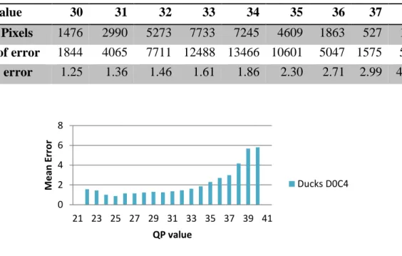
The data contained the sum of errors, between the original pixel value and the reconstructed pixel value, for all pixels with different QP values in each block. It also contained the number of pixels having a certain QP. From the data, the absolute value of the sum of errors was summed up for all blocks in a frame, within each direction and category. The sum was divided by the total number of pixels in the frame with corresponding QP to give the total mean error for each QP. See example of data in Table 2. Graphs were plotted based on these calculations, see example Figure 8. All graphs pointed to an increase of error for QP values above around 32, the average QP value of all the pixels in the frame. This indicated that there were a correlation between the QP value and the mean error.

Table 2. Data extracted from DucksTakeOff, direction 0, category 4.

QP Value 30 31 32 33 34 35 36 37 38 Nr of Pixels 1476 2990 5273 7733 7245 4609 1863 527 120

Sum of error 1844 4065 7711 12488 13466 10601 5047 1575 501

Mean error 1.25 1.36 1.46 1.61 1.86 2.30 2.71 2.99 4.18

Figure 8. Graph representing mean error based on QP value, from DucksTakeOff, direction 0, category 4

3.2.2 Model correlation

As mentioned, in the original SAO filter the offsets correspond to an integer value B, in the range of -7 to 7 that reduces the error the most. However, in the QP-based SAO the offset is the resulting value of a model that is dependent on both the B value and the QP value of the current pixel. Since the pixel values are integers, the resulting offset of the model is rounded off to the closest integer value to be applicable. A linear function

0 2 4 6 8 21 23 25 27 29 31 33 35 37 39 41 M e an E rr o r QP value Ducks D0C4

(22)

17

𝑜𝑓𝑓𝑠𝑒𝑡 = 𝑟𝑜𝑢𝑛𝑑(𝐵 + 𝐵 × (𝑄𝑃 − (𝑎𝑣𝑄𝑃 + 𝐶)) × 𝐾), (6)

was investigated as model. When the model is used, different B values are tested, and the one providing the least error will be selected. The constant 𝑄𝑃 is the QP value of the current pixel. 𝑎𝑣𝑄𝑃 is the value of the average QP values of all the pixels in the current frame, which means that the avQP value will change for each new frame. C and K are parameters which might be constant or vary for each frame. They are adjusted in order to fit the model to the data.

Since all the QP values for one frame lie within a limited span, what can be called the origin of the model was placed within that span. Since avQP certainly has a value within the limit it was set as a part of the origin value, and the integer C was added so the best value for it could be estimated. When the QP value of the current pixel equals the value of avQP + C, the second term in Equation 6 is set to zero. In that case the offset corresponds to the integer value B. Therefore, the value of C directly affects how well the model can fit the data. The K parameter was added to the second term of the model in order to adjust the slope, and since the offset is expected to increase with higher QP values it is restricted to a positive value. The B value was also multiplied with the latter part of the equation so that in case the selection of B was zero, no offset is applied.

Other models, such as an exponential, were also considered. However, only the linear model was evaluated further. If more time had been available the exponential model would have been investigated as well.

3.2.3 Obtaining parameters for QP-based SAO

In order to find the values of parameters C and K in the model given in Equation 6, an implementation in the SAO filter was done. The implemented algorithm let different B values be tested for set values of C and K in the model, where the B providing the least error was selected, as it would in the final implementation. This way, the error reduction the model provided with different combinations of C and K was calculated for a whole frame. The errors in the SAO filter with the QP-based SAO model are calculated as the square of the difference between the original pixel value and the reconstructed pixel value. Hence, the error reduction the model provided was the error obtained when no SAO filter was used, subtracted by the error obtained when using the QP-based SAO model. The error reduction provided by the reference encoder with mode 2 was also calculated for comparison. Calculations were made on five different sequences, with QP 27 and QP 37 to see if there would be any difference for best values of C and K, dependent on which QP value the sequences were coded with. The first frames of the videos were used for the calculations, which added up to 2200 blocks. The output showed how much bigger error reduction, in percent, different C and K values for the model gave, compared to the error reduction by mode 2. The C and K values that provided the biggest error reduction in the different sequences indicated their final values to be implemented in the model, see results in section 4.3. There was a

(23)

18

possibility that different combinations of C, K and B could result in the same model which would provide the same error reduction. However, this possibility was eliminated since the costs of signaling B values were computed into the error, so that a smaller B value would provide a smaller error than a larger one. The calculation of the cost of signaling B values are further described in section 3.2.5.

3.2.4 Functionality of the QP-based SAO

When the parameters C and K have been found, the model is implemented with their values set for each frame. avQP is retrieved for the current frame and QP for the current pixel. The possible B values are tested and the one giving the least total error for each direction and category is chosen. In Figure 9, a graph shows how different values of B can result in different offset values for the model, where the rest of the parameters are defined, which is how it will be when the model is implemented. In Figure 9 the parameters avQP = 30, C = 2, and K = 0.1 are chosen arbitrary for the sake of the example.

Figure 9. Graph showing possible offsets for different QP values, dependent on which B value that is selected for the model.

3.2.5 Implementation of QP-based SAO

In c65, the parameters for the original SAO filter are calculated in a function called compress(). It loops through each 64 sized block in a frame, where it goes through all four directions and sorts the pixels into the category it belongs to for the current direction. The sum of errors from all pixels and the number of pixels in each category get stored. The errors are calculated by the original pixel value subtracted by the reconstructed value, showed in equation 8.

𝐸𝑟𝑟𝑜𝑟 = 𝑜𝑟𝑖𝑔𝑖𝑛𝑎𝑙 − 𝑟𝑒𝑐𝑜𝑛𝑠𝑡𝑟𝑢𝑐𝑡𝑒𝑑. (8) 0 0.5 1 1.5 2 2.5 3 3.5 4 4.5 29 30 31 32 33 34 35 Of fs e t

QP value of current pixel

B=1 B=2 B=3

(24)

19

So if the reconstructed pixel value is less than the original, the error is positive, and if it is bigger, the error is negative. From this, the direction that gives the biggest error reduction is chosen and the offsets are calculated. If the reduction in error is bigger than the cost of sending the offsets for all four categories, the SAO filter is used and the offset values are added to all pixels in the categories respectively.

The QP-based SAO algorithm was implemented as an alternative to compress() and it works in the same way, by looping through the blocks and categorizing the pixels. When storing the squared error, the model is added as

𝐸𝑟𝑟𝑜𝑟 = (𝑜𝑟𝑖𝑔𝑖𝑛𝑎𝑙 − (𝑟𝑒𝑐𝑜𝑛𝑠𝑡𝑟𝑢𝑐𝑡𝑒𝑑 + 𝑟𝑜𝑢𝑛𝑑(𝐵 + 𝐵 × (𝑄𝑃 − (𝑎𝑣𝑄𝑃 + 𝐶)) × 𝐾)))2 (9) The possible B values are tested and the one giving the least total error for each direction and category is chosen. This is done to obtain the best offsets for when the model will be applied, in a later stage. Additionally, the cost of signaling the B value and its sign is added to the error, in order to take the rate distortion impact into account. The cost of signaling the B value is calculated by multiplying λ from RDO for the current CTU, with the absolute value of the B value. Hence, bigger values of B are penalized. The non-zero B values also added the value of λ to the error, to consider the cost of signaling the sign. This is an approximation of the true signaling cost which also depends on the states of the CABAC encoder. The direction giving the biggest reduction in error, by using selected offsets compared to not using them, is chosen. Thereafter, the decision if the SAO filter should be applied for the current block is made in the same way as for the original algorithm. When applied, the B values chosen for each category are signaled, and the resulting offset values they provide from Equation 6 are added to each pixels reconstructed value, as

𝑛𝑒𝑤𝑅𝑒𝑐𝑜𝑛𝑠𝑡𝑟𝑢𝑐𝑡𝑒𝑑 = 𝑟𝑒𝑐𝑜𝑛𝑠𝑡𝑟𝑢𝑐𝑡𝑒𝑑 + 𝑜𝑓𝑓𝑠𝑒𝑡. (10)

3.3 Reference encoder

In the QP-based SAO implementation the offsets are chosen optimally, since all the possible B values and the corresponding error is calculated. The original SAO implementation only gives an estimate of the optimal offsets which means that its performance cannot be correctly compared to the QP-based SAO. To enable the use of the original SAO in a reference encoder an implementation where the original SAO filter could use optimal offset selection was done. This was done in the same way as in the QP-based SAO, by looping over all possible offset selections and calculating the errors. Simulations with the original SAO algorithm compared to the original SAO algorithm, but with optimal offset selection were conducted. As expected, the results showed a slight improvement with optimal offsets. This led to the conclusion that an encoder with the QP-based method could correctly be compared to one with original SAO but optimal offset selection, see section 4.2. From now on, when needed, the different SAO implementations are referred to as follows:

(25)

20

 Mode 1: The original SAO algorithm to calculate the offsets

 Mode 2: The original SAO algorithm to calculate the offsets, with optimal selection of the offsets

 Mode 3: The QP-based SAO algorithm to calculate the offsets, with optimal selection of the offsets

Where mode 2 is the reference encoder which mode 3 with the QP-based SAO method is compared to.

3.4 Test sequences and simulation process

All video sequences used for data and simulations in this project were provided by Ericsson. All test sequences are stored as raw video files, with YUV 4:2:0 colour sampling, and 8 bits per sample. When testing the implementation of QP-based SAO, objective measurements were used. Since the possible gain would only reach about one single percent it would not be noticed subjectively.

When performing objective performance tests of the implemented techniques, videos and conditions were used according to the JCT-VC document Common test conditions

and software reference configuration [24]. The videos included in the Random Access

set were used, except the videos from class A with 10 bits per sample. This test set is referred to as the JCT-VC test set.

The sequences were coded with the four different QP values; 22, 27, 32 and 37, as advised in the JCT-VC document. I-frames were set to every 48th picture, and the coding was hierarchical with P-frames every 8th picture. Simulations were made when all frames in a sequence had mode 3 applied. Additionally, simulations where made with only the I-frames coded with mode 3 and the rest with mode 2. In the simulations there is always a reference encoder set as an anchor. This means that the performance of the tested encoder will be evaluated in comparison to the performance of the anchor. The parameter which is used for evaluation of the simulations is the BD rate, which as mentioned includes evaluation of PSNR and bitrate and is referred to as compression efficiency. In the results, the BD rates for Y, U and V, stands for luma, chroma blue, and chroma red respectively. The results for Y are the most important, since HVS is more sensitive to brightness than color.

The five video sequences used for obtaining C and K were selected randomly. However, all had resolution 1280 x 720 in order to provide more data than a lower resolution would have. They also had different characteristics and only one of them is included in the final simulation JCT-VC test set. The JCT-VC test set is sufficiently varied in characteristics that no algorithm should be able to be optimized just for it. However, using this unrelated group of sequences ensured that the model would not be optimized in a beneficial way just for the JCT-VC test set.

(26)

21

4. Results and discussion

In this section, both results from the working process and final simulations are presented and discussed.

4.1 Subjective evaluation of VAQ

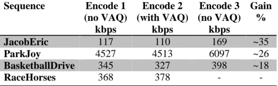
In table 3 the resulting bitrate sizes from videos coded with and without VAQ are shown. The sequences JacobEric and ParkJoy were selected since both have areas where VAQ were expected to perform well. BasketballDrive and RaceHorses were chosen at random. Firstly, all sequences were coded with a set QP without VAQ. When the sequences are coded, video files for subjective evaluation are created. Thereafter, the sequences were coded with VAQ. To enable a first comparison between the coded sequences, the bitrate of the sequence coded with VAQ should be similar to the one coded without VAQ. Therefore, the sequences with VAQ were coded with different QP values until a video file of similar bitrate as the previously coded video file was found. By subjective evaluation of the sequences, the first three videos in the table had notably better quality in the sequence coded with VAQ. In the last sequence no difference could be spotted. The sequences were coded without VAQ one more time. This time, with decreasing QP value, until the same perceived quality as with VAQ was obtained. In all three cases the encoder with VAQ could represent the same video quality with lower bitrate. In the first sequence the gain was 35%, which means that by coding with VAQ the video can be represented with the same subjective quality as without VAQ, but with 35 % lower bitrate. However, since the videos could not be compared with identical bitrate, and since the subjective evaluation is based on personal opinion, the percentages are only approximate. For both Jacoberic and ParkJoy the results confirm the suitability of VAQ for videos with parts having distinct texture but low variance. In Figure 10, screenshots from JacobEric from Encode 1 and Encode 2 are displayed. The picture from Encode 2 shows better subjective quality with a more defined beard and clearer lines around the mouth. Separate frames from all the videos are shown in Appendix A, where links to some of the clips can be found as well. These results verified the functionality of VAQ in c65.

Table 3.Video sequences coded with and without VAQ and their corresponding bitrate. Encode 1 and 2 have similar bitrates, while 2 and 3 have same subjective quality.

Sequence Encode 1 (no VAQ) kbps Encode 2 (with VAQ) kbps Encode 3 (no VAQ) kbps Gain % JacobEric 117 110 169 ~35 ParkJoy 4527 4513 6097 ~26 BasketballDrive 345 327 398 ~18 RaceHorses 368 378 - -

(27)

22

Figure 10. Screenshots from JacobEric from Encode 1 and Encode 2. Encode 2, to the right, with the VAQ technique provides a better subjective quality.

4.2 Verifying reference encoder

The performance of mode 2 was evaluated against mode 1, to verify that mode 2 with optimal offset selection had better objective performance than mode 1. If so, mode 2 could be used as a reference encoder when evaluating the objective performance of mode 3 with the QP-based SAO model. The average BD rate Y for all the sequences in the test set were -0.57 % as shown in Table 4. This means that mode 2 on average is able to encode the videos with a 0.57 % reduction in bitrate while retaining the same video quality as in mode 1. This implies, as expected, that the optimal selection of offsets in mode 2 is slightly beneficial to the estimation of optimal offset in mode 1. Since the SAO filter in total stands for a three to four percent average gain, a 0.57 % gain is big enough to conclude that offset selection of mode 2 is beneficial. Therefore, mode 2 worked as an anchor when evaluating the objective performance of mode 3. The encoding time of mode 2 is 11 % longer than for mode 1, which most likely is caused by the optimal selection of offset in the SAO filter, where it loops through all possible selections.

Table 4. Performance in BD rate of mode 1 compared to mode 2.

Mode 2 vs Mode 1 BD rate Y % BD rate U % BD rate V % Encoding time % JCT-VC test set -0.57 -0.17 -0.12 11

4.3 Obtaining C and K for the QP-based SAO model

To find which C and K values that were suitable for the QP-based SAO model, the error reduction the QP-based model provided compared to not using the SAO filter was calculated. This was done for a range of possible K and C values, and compared in percent, to the error reduction provided by mode 2. The process is described in more detail in section 3.7. One example of the resulting percent for different combinations of C and K, calculated for one sequence, is shown in Figure 11. It shows a graph where the error reduction percent of the C and K values is indicated by color. For example, in

(28)

23

Figure 11, C = 0 and K = 0.1 gave the largest error reduction for that sequence, a 7% larger error reduction than mode 2. The combination of C and K that provided the biggest error reduction, gave for all sequences a larger reduction than mode 2. In videos coded with lower QP, the error reduction was in general larger than in videos coded with larger QP value. In Table 7, the C and K values that provided the biggest error reduction for the first frame in the different sequences are shown, as well as the avQP for the frame and the resulting avQP + C value. Calculations were made for the sequences coded with QP 27 and QP 37 to see if that influenced which K and C values gave the most error reduction.

Figure 11. Graph showing how much bigger error reduction in percent different combinations of K and C provides, compared to mode 2, for sequence ParkJoy, coded

with QP 37. The larger the error reduction, the brighter the color.

Table 7. C and K values giving biggest error reduction for different sequences coded with two different QP values. avQP for the frame and the resulting avQP + C value are

displayed as well.

Sequence Coded with QP avQP K C avQP + C Wisley 27 18 0.05 12 30 ChristmasTree 27 19 0.06 12 31 BasketballDrive 27 23 0.05 10 33 DucksTakeOff 27 23 0.05 10 33 ParkJoy 27 24 0.06 9 33 Wisley 37 28 0.06 6 34 ChristmasTree 37 29 0.1 1 30 BasketballDrive 37 33 0.1 0 33 DucksTakeOff 37 33 0.1 0 33 ParkJoy 37 34 0.1 0 34

(29)

24

When the coded QP, hence the avQP for the frame increased, the K values that gave more error reduction seemed to increase as well. This indicated that K could be dependent on avQP. The C values seemed to decrease with increased avQP, which meant that avQP + C for all the sequences resulted in similar values. Based on these results, avQP + C was tested as a constant value. The mean values of avQP + C for all the sequences is 32.4, so both 32 and 33 were tested. The K variable was defined as a line dependent on avQP from least square method, Figure 12 and corresponding model:

𝐾 = 0.004 × 𝑎𝑣𝑄𝑃 − 0.02. (11)

Separate frames from the videos in Table 7 are shown in Appendix B, where links to some of the clips can be found as well.

Figure 12. K values by avQP for different sequences, and the corresponing fitted linear

model.

4.4 Evaluating the performance of QP-based SAO

A simulation was made with the JCT-VC test set to evaluate how mode 3 with the QP-based SAO model performed compared to the reference encoder. Setting avQP + C to 32 had worse compression efficiency than when set to 33. The result for when the latter was implemented in mode 3, compared to the anchor mode 2, is shown in Table 8. A table of all results for the individual sequences in the JCT-VC test set can be found in Appendix C. A positive BD rate indicates a worse compression performance of the tested encoder compared to the anchor, which means that mode 3 seemed to perform worse than mode 2, but slightly better when only used on I-frames. When only used on I-frames the average BD rate Y for all the sequences in the JCT-VC test set was 0.008%. This means that mode 3 requires a 0.008% higher bitrate to provide the same objective quality as mode 2. However, an average BD rate for the test set of that magnitude is insignificant. Furthermore, in the results for each sequence in the test set, mode 3 has a negative BD rate compared to mode 2 for 8 out of the 19 sequences. Therefore, no conclusion if mode 3 has better or worse compression efficiency than mode 2 can be made.

0 0.02 0.04 0.06 0.08 0.1 0.12 17 22 27 32 K avQP K Linear (K)

(30)

25

Table 8. Performance in BD rate of mode 2 compared to mode 3, with VAQ.

It was gathered that the λ coefficient that is used for adding the cost of signaling the offsets could affect the results negatively. It is dependent on the RDO, and is calculated from the current QP in the CTU. When VAQ is implemented, higher QP values are assigned to areas where bigger errors are allowed since they will not affect the visual perception negatively, but they will lower the PSNR. If a CTU has a high QP value the λ coefficient gets bigger. The SAO filter offsets are signaled only if the error is reduced with more than the value of λ. Therefore, it could be that the error reduction applied by the SAO will not be big enough for CTUs with higher QP values, and no offsets will be applied. On the contrary, offsets might be more likely to be applied in blocks with lower QPs. The effect of VAQ will in a sense be enhanced, and since it increases the subjective quality and not PSNR/BD rate, that could explain the results. To see if above speculations may have affected the results for VAQ, the VAQ algorithm was turned off.

When VAQ is turned off the QP values that are assigned to different blocks provide higher PSNR. To be able to take these QP changes within a CTU into account, the rate distortion impact as calculated before, with λ for the whole CTU, does not work. Instead, the lambda is retrieved for the smallest size it can be retrieved from, size 16. By dividing the calculated errors in SAO with λ for each 16 block, the errors are weighted depending on the QP changes, which should provide the best possible BD rate.

These changes in implementation were done in mode 2 and mode 3. Mode 2 was once again tested against mode 1 to verify its optimal selection of offsets. This time it performed 0.39 % better in BD rate Y compared to mode 1. That result led to the same conclusions as in section 4.2, and mode 2 was verified as reference encoder. With the changes of the implementation in mode 3, new parameter selections of C and K were made. In table 9, the C and K values that provided the biggest error reduction for the first frame in the different sequences are shown, as well as the avQP for the frame and the resulting avQP + C value.

Mode 3 vs Mode 2 With VAQ Only Intra frames BD rate Y % BD rate U % BD rate V %

JCT-VC test set Yes 0.008 0.019 -0.054

(31)

26

Table 9. C and K values giving biggest error reduction for different sequences coded with two different QP values. avQP for the frame and the resulting avQP + C value are

displayed as well.

Sequence Coded with QP avQP K C avQP+C Wisley 27 18 0.07 12 30 ChristmasTree 27 19 0.07 11 30 BasketballDrive 27 23 0.06 7 30 DucksTakeOff 27 23 0.07 6 29 ParkJoy 27 24 0.05 8 32 Wisley 37 28 0.05 9 37 ChristmasTree 37 29 0.04 10 39 BasketballDrive 37 33 0.03 5 38 DucksTakeOff 37 33 0.05 4 37 ParkJoy 37 34 0.04 4 38

As before, both the C and K values seemed to change with avQP. The avQP + C values did not result in similar values but increased with avQP as well. Therefor both C and K seemed to depend on avQP. Their values and how they relate to the avQP of the frame of the sequence are shown in graphs, Figure 13 and 14. C and K was estimated by avQP using least square, and are shown as straight lines in the same figures, and described as

𝐶 = 18 − 0. 4 × 𝑎𝑣𝑄𝑃, (12)

𝐾 = 0.11 − 0.002 × 𝑎𝑣𝑄𝑃. (13)

When the variables are implemented in the QP-based SAO model, the C is rounded to the closest integer value.

Figure 13. avQP + C values by avQP for different sequences, and the corresponing

fitted linear model. 25 30 35 40 17 22 27 32 av QP + C avQP avQP + C Linear (avQP + C)