ANALYTICAL METHODS FOR CHARACTERIZING OIL AND GAS DEVELOPMENT AND PRODUCTION WASTE STREAMS: A CRITICAL REVIEW AND
COLLABORATIVE INTER-LABORATORY COMPARISON
by
ii
A thesis submitted to the Faculty and the Board of Trustees of the Colorado School of Mines in partial fulfillment of the requirements for the degree of Master of Science
(Environmental Science and Engineering)
Golden, Colorado Date _____________
Signed: __________________________ Bethany Grace Yaffe Signed: __________________________ Dr. Tzahi Cath Thesis Advisor Golden, Colorado Date _____________ Signed: __________________________ Dr. John McCray Professor and Department Head Department of Civil and Environmental Engineering
iii
ABSTRACT
As the oil and gas industry expands in the United States, managing the high volume waste streams generated during development and production becomes increasingly crucial to the preservation of ecosystem and human health. Accurate characterization is essential to ensure proper treatment and disposal. Therefore, a collaborative inter-laboratory comparison was performed using methods applied to oil and gas development and production wastewaters. Four samples were analyzed using five different methods. The samples included raw fracturing flowback, treated fracturing flowback, raw produced water, and treated produced water. The methods used to characterize these waters were EPA Method 300.0, EPA Method 200.7, EPA Method 200.8, SW 846 Method 6010C, and SW 846 Method 8015B.
The mean, standard deviation, and relative standard deviation of the results from this inter-laboratory comparison were compared to the mean, standard deviation, and relative standard deviation found in each of the EPA methods validation data. This comparison elucidated the variation resulting from the application of the EPA methods to the oil and gas development and production wastewater matrices.
iv TABLE OF CONTENTS ABSTRACT ... iii TABLE OF FIGURES ... v TABLE OF TABLES ... vi ACKNOWLEDGMENTS ... vii DEDICATION ... viii CHAPTER 1. INTRODUCTION ... 1
1.1 Oil and gas development and production waste streams ... 1
1.2 Treatment and disposal ... 3
1.3 Regulation of oil and gas development and production waste streams... 3
1.4 Analytical methods for oil and gas wastewater ... 5
CHAPTER 2. MATERIALS AND METHODS ... 7
2.1 Sample preparation ... 7
2.2 Analytical methods ... 7
2.3 Determination of inorganic anions by ion chromatography (IC): EPA method 300.0 ... 8
2.4 Determination of metals and trace elements in water and wastes by inductively coupled plasma – atomic emission spectrometry (ICP-AES): EPA Method 200.7 and SW 846 Method 6010C.cb ... 10
2.5 Determination of trace elements in waters and wastes by inductively coupled plasma – mass spectrometry (ICP-MS): EPA Method 200.8 ... 10
2.6 Nonhalogenated organics using gas chromatography/flame ionization detector (GC-FID): SW 8015B ... 11
2.7 Quality assurance ... 13
CHAPTER 3. RESULTS AND DISCUSSION ... 15
3.1 Performance by anion ... 15
3.2 Performance by cation ... 19
3.3 Total Petroleum Hydrocarbons ... 26
CHAPTER 4. CONCLUSION ... 33
REFERENCES CITED ... 35
APPENDIX A: QUALITY ASSURANCE / QUALITY CONTROL OF THE INTER-LABORATORY COMPARISON ... 39
APPENDIX B: CHARACTERIZATION OF THE OIL AND GAS DEVELOPMENT AND PRODUCTION WASTEWATER SAMPLES ... 43
APPENDIX C: METHODS APPLICABLE TO OIL AND GAS DEVELOPMENT AND PRODUCTION WASTEWATERS ... 48
v
LIST OF FIGURES
Figure 1. The Linear Calibration Range (LCR) as calculated by New Mexico State University for this inter-laboratory comparison. The LCR must be verified every six months as required by EPA Method 300.0. ... 9 Figure 2. Five anions analyzed in the four oil and gas wastewater streams. The horizontal tick labels represent the number of results that were reported as detectable concentration for the anion. Aluminum chloride was used as a coagulant, slightly increasing chloride levels in the treated produced samples. ... 18 Figure 3. Cations found in oil and gas development and production wastewaters, both before and after treatment. The horizontal tick labels represent the number of results reported as a detectable concentration of the cation... 20 Figure 4. Analytical results for the major cations found in both the treated and untreated oil and gas development and production wastewaters. The horizontal tick labels represent the number of analytical results available for the cations. ... 21 Figure 5. Chromatogram of the raw fracturing flowback extraction. The DRO elute between 5.53 and 14.18 minutes. The ORO elute between 14.18 and 23.20 minutes. The majority of the organics found in raw fracturing flowback are between C8 and C33. ... 27 Figure 6. Chromatogram of the treated fracturing flowback extraction. The DRO elute between 5.53 and 14.18 minutes. The ORO elute between 14.18 and 23.20 minutes. The majority of the organics found in treated fracturing flowback are between C8 and C20, with the only substantial peak being C20. ... 28 Figure 7. Chromatogram of the raw produced water extraction. The DRO elute between 5.53 and 14.18 minutes. The ORO elute between 14.18 and 23.20 minutes. The majority of the organics found in raw produced water are between C8 and C20, with the only substantial peak being C20. .... 29 Figure 8. Chromatogram of the treated produced water extraction. The DRO elute between 5.53 and 14.18 minutes. The ORO elute between 14.18 and 23.20 minutes. The majority of the organics found in treated produced water are between C8 and– C20, with the only substantial peak being C20. After treatment, many diesel range organics remain in the produced water. ... 30
vi
LIST OF TABLES
Table 1. Analytical methods used in this inter-laboratory comparison, along with the analytes chosen for analysis. Each laboratory performed the following analysis on four different samples, including pretreated produced water, raw produced water, pretreated fracturing flowback, and raw fracturing flowback. ... 8 Table 2. Summary of RSD values for the anions that displayed the highest variability in analysis compared to the RSD values as reported by EPA Method 300.0. The matrices are raw fracturing fluid (RFF), treated fracturing flowback (TFF), raw produced water (RPW), and treated produced water (TPW). ... 17 Table 3. Summary of RSD values for the cations that displayed the highest variability in analysis compared to the RSD values for the three methods used to analyze cations in this inter-laboratory comparison. The matrices are raw fracturing fluid (RFF), treated fracturing flowback (TFF), raw produced water (RPW), and treated produced water (TPW). ... 24 Table 4. Summary of GC/FID results for combined diesel and oil range organic concentrations (mg/L) from participating laboratories for raw fracturing flowback (RFF), treated fracturing flowback TFF), raw produced water (RPW), and treated produced water (TPW). The missing cells represent analysis that were unsuccessful due to inadequate volume. The laboratories that reported EPH concentrations were Accutest (ACC), Stewart Environmental (SE), and University of Colorado, Boulder (CUB). CUB n.1 is the first round of analysis, with the n representing the replicate number, and CUB n.2 is the second round of analysis. ... 27 Table 5. GRO concentration in mg/L as analyzed by Accutest (ACC) and Stewart Environmental (SE) for the raw fracturing flowback (RFF), treated fracturing flowback (TFF), raw produced water (RPW), and treated produced water (TPW)... 32
vii
ACKNOWLEDGMENTS
Without the help of many people, this thesis would not be possible. Primarily, I would like to thank my adviser, Dr. Tzahi Cath, who spent many hours helping me problem solve, editing my work, and guiding me through the maze that this project became. I would also like to thank Dr. Dean Heil, Bryan Coday, and Dan Freedman, who were always willing to give me help and guidance.
I must also thank the professors and graduate students at the universities that participated in this inter-laboratory comparison. Thank you to Dr. Pei Xu from New Mexico State University, Dr. Jonathan Brant from University of Wyoming, Dr. Brian Majestic from the University of Denver, Dr. Jason Ren from the University of Colorado, Boulder, Dr. Karl Linden from the University of Colorado, Boulder, and Dr. Eric Dickenson from the Southern Nevada Water Authority. Thank you Benton Cartledge, Casey Forrestal, and James Rosenblum for the hard work you put in toward this project. Thank you to Michael Glavanovich at Stewart Environmental and Renea Jackson and Cristina Berrutti at Accutest for answering my many questions.
Thank you to my family and friends that might as well be family for the many hours of baby-sitting, house cleaning, and food delivering that you selflessly gave me as I worked toward completing my Master’s. You were always there for me when I needed you, and I am eternally thankful. This accomplishment is just as much yours as it is mine, for I could never have made it this far without your love and support.
viii
DEDICATION
For my sons, Asher and Azariah. You will always be my heart, inspiration, motivation, and best teachers. Your excitement to learn encourages me to ask why, your desire to help encourages me to leave a better world, and your trust encourages me to give everything I have.
With all my love and everything I am, Mommy.
1
CHAPTER 1 INTRODUCTION
The management of water resources faces considerable challenges as the oil and gas industry in the United States continues to expand in response to recent energy independence policies, advancements in hydraulic fracturing, and the growing energy demand. Both water consumption and water quality management are crucial to the sustainability of the oil and gas industry. Impacts to water quality in many oil and gas producing regions are of great concern as oil and gas development and production have the potential to contaminate surface and groundwater resources. Drilling operations, improper disposal of produced and flowback water, abandoned wells that are inadequately sealed, malfunctioning equipment, vandalism, and accidental releases of both crude oil and produced and flowback water have all been sources of surface and groundwater contamination in the past [1].
1.1 Oil and gas development and production waste streams
Oil and gas development and production operations require large volume of freshwater and generate even larger volumes of wastewater in the form of drilling mud, hydraulic fracturing flowback, and produced water. Drilling fluid, synonymous with drilling mud, encompasses most fluids that are used in hydrocarbon drilling operations. They are necessary to cool and lubricate the drill string and the wellbore during drilling operations, as well as remove drilled solids and convey them to the surface [2]. However, drilling fluid is not included in this study and will not be discussed further. The main focus of this research is on fracturing flowback and produced water, two major waste stream generated by the oil and gas industry. During hydraulic fracturing (fracking), water mixed with various chemical additives is injected at high pressure into a tight rock formation to fracture the rock and allow for the free flow of hydrocarbons to the well, and from the well to the surface [3, 4]. Fracking additives include proppants (i.e., sand or other hard particles used to keep the well fractures open), guar gum or other gels, biocides, surfactants, corrosion inhibitors, and scale inhibitors [5]. During each pumping/fracturing stage, 2 to 12 million gallons of water, of which less than 1% is typically comprised of chemical additives, is injected into the oil or gas baring
2
formation. These pumping stages may last between 20 minutes to 4 hours, [5]. Depending on the physical properties of the subsurface formation, typically, 10-40% of the fracturing fluid is unrecoverable because it enters pore spaces in the formation [6]. Following well fracturing, flowback of the fracturing fluid mixed with formation water may last two to three weeks beginning at the rate of 125 to 150 gallons per minute, and then dropping to an average rate of approximately 30 gallons per minute [6]. Over time, produced water, or water that is found in the oil or gas reservoir, will begin to flow out of the well with the fracturing flowback, changing the character of the flowback stream to what is found naturally in the reservoir rock.
Produced water is the water that flows out of the well with the oil and gas during production. It may be composed of multiple sources such as connate water (i.e., water trapped by capillary pressure in the local rock formations), water from aquifers below the oil reservoir, and waterflood water [2]. Waterflood water originates from an injection of water into the oil formation with the goal of displacing residual oil and encouraging subsequent flow to the surface [7]. The chemical characteristics of produced water is highly variable between the type of fossil fuel resource being developed (i.e.,. conventional vs. unconventional) and from basin to basin [8]. Produced water is a complex matrix of both naturally occurring constituents and additives, and contains dissolved inorganic and organic compounds, residual development fluids, and treatment chemicals. This vast array of elements and compounds may consist of minerals, ions, non-hydrocarbon dissolved gasses, radioactive materials, soluble hydrocarbons, gases, carboxylic acids, scale control additives, corrosion inhibitors, and biocides [7-9].
Produced water leaves the formation with the upcoming oil or gas, and requires removal of the freestanding oil prior to storage. During flow from treatment to storage, oil droplets remaining in the water become highly emulsified as the water passes through valves and pumps. Additionally, corrosion inhibitors stabilize the oil-in-water dispersion [10]. These two factors combined complicate subsequent water treatment processes [7].
3
1.2 Treatment and disposal
Management of flowback and produced waters is economically driven within the regulatory confines of local and federal jurisdictions [11]. Current management practices include temporary onsite storage followed by transportation for offsite disposal, either by deep well injection or treatment for industrial reuse, or indirect surface water discharge [3, 12]. In most areas, deep well injection is the primary method of wastewater disposal because it requires little or no treatment and is often the most economical option [3, 11]. In cases where treatment is either cost-competitive or required by regulations, challenges exist in rendering the waste streams amenable for surface water discharge or onsite reuse. Typical challenges include removal of oil and grease, suspended solids and heavy metals precipitation, removal of soluble organics, softening, and desalination [8, 13, 14]. There are some treatment options available to manage these target constituents, including physical, biological, and chemical processes [13-20].
In a typical treatment scheme, the fracturing flowback or produced water first undergoes primary de-oiling using gravity based processes such as skimming and gravity separators. After primary de-oiling, the water passes through a secondary de-oiling treatment such as flocculation, or gas flotation. Subsequent tertiary treatment may be used to remove fine particles through filtration or centrifuge processes [7]. After treatment, the water might be considered acceptable for reuse in subsequent fracturing operations.
1.3 Regulation of oil and gas development and production waste streams
Deep well disposal and surface water discharge are monitored and regulated by the United States Environmental Protection Agency (USEPA). Currently, there is no national standard regulating the disposal of oil and gas development and production wastewater. There are, however, some federal regulations authorized by the National Pollution Discharge Elimination System (NPDES) as authorized by the Clean Water Act (CWA; 40 CFR Parts 122 through 125). The Effluent Limitations Guidelines (ELGs) for the NPDES for oil and gas point source discharges are regulated under 40 CFR 435. Under these regulations, direct disposal of oil and gas wastewater is not allowed into any US navigable water, and possible accidental release, an example of which would be through storm water runoff, is highly regulated through the NPDES
4
permitting system. Additionally, the discharge may also be regulated by the state in which the permit is granted.
Indirect discharges from Publically Owned Treatment Works (POTW) are allowed, and are subject to the General Pretreatment Regulations (40 CFR Part 403). While this treatment method is uncommon, it has been used in the Marcellus shale play in Pennsylvania and in Wyoming [21, 22]. As POTW’s do not have the capability to treat the high salinity and radioactivity of the water, this practice has led increased levels of chloride, bromide, and radium in receiving surface waters and sediments. The increase in downstream TDS has in turn raised concerns of brominated disinfection products in downstream drinking water treatment facilities [21].
Currently, the only oil and gas development and production wastewater that is unregulated is coalbed methane production water [23]. During the development of the ELGs, coalbed methane was not being widely extracted; therefore, the EPA did not consider this wastewater in the original discharge permitting. Thus, NPDES permits for coalbed methane discharge is based on best professional judgment (BP) as outlined by 40 CRF 125.3(c)(2), and can vary significantly between states. In some cases, this water has been directly discharged to surface water following minimal treatment [24].
To mitigate the risks associated with indirect surface water discharge, deep well injection is the preferred method of disposal for oil and gas development and production wastewaters. This process is regulated under the Safe Drinking Water Act’s Underground Injection Control (UIC) program as outlined in 40 CFR 144-148. Oil and gas regulated injection wells, or Class II wells, are wells that allow for the injection of wastewaters resulting from oil and gas development and production. There are over 172,068 Class II operational wells in the US today, receiving over two billion gallons of wastewater every day [25]. However, certain areas in the US either lack adequate access to deep well injection sites, or deep well injection is banned in the area, leading to the necessity of either treatment and reuse or surface water discharge [21]. Pennsylvania is an example of an area that is lacking access to deep well injection, resulting in use or POTW and indirect surface water discharge [21, 26].
5
1.4 Analytical methods for oil and gas wastewater
The main driving force in correct characterization of oil and gas wastewaters are the negative impacts possible with indirect surface water discharge [8]. The discharge of these wastewaters into waterways is heavily regulated under the NPDES permitting system, requiring adherence to daily maximum effluent limitations and including an understanding that the effluent is not hazardous to humans, wildlife, or livestock. However, the toxicity of the water cannot be properly understood without a correct characterization of the water.
Currently, there are no methods specifically outlined for the analysis of oil and gas development and production wastewater, which can lead to variations in analytical results and detection limits [2]. Commercial laboratories use EPA, American Society for Testing and Methods (ASTM), or Standard Methods (SM) methods in the analysis of oil and gas wastewater, with the vast majority favoring EPA methods. Disposal of these wastewaters is regulated through the EPA, requiring adherence to their approved methods. Within the oil and gas industry, the American Petroleum Institute (API) has internal standard methods; however, EPA methods must be used for regulatory purposes. A list of methods used for analysis of oil and gas development and production wastewater is provided in Appendix C.
Constituents of produced and flowback water make the matrix uniquely difficult to analyze. High concentrations of calcium, magnesium, sodium, chloride, fluoride, emulsified oil and grease, and fine particulate matter are known to cause analytical interference, clog sensitive instruments, and yield inconsistent results. To mitigate any potential difficulty with sample analysis, the samples may be digested, filtered, and diluted before analysis. However, additional errors in analysis may result from these sample preparation methods. In particular, dilution greatly diminishes the ability to measure trace constituents in the sample.
Even with the consistent use of EPA testing methods across commercial laboratories, different EPA methods are often used to characterize the same analytes. For example, methods associated with the Clean Water Act (such as EPA Method 200.7 and 200.8) or Solid Waste (SW 846) Methods may be used to determine the total recoverable cations (for example SW 846 6010C). Furthermore, different preparation
6
methods may be used (such as SW 846 3010 and EPA 3052). In addition to the variability of methods used, methods are often altered, as many are not able to handle the unique make-up of produced and flowback water.
The main objective of this study was to explore the methods used to analyze produced and fracturing flowback wastewater and to evaluate the differences in analytical results. This goal was carried out through an inter-laboratory comparison of four oil and gas development and production wastewaters, including raw fracturing flowback, treated fracturing flowback, raw produced water, and treated produced water.
7
CHAPTER 2 MATERIALS AND METHODS
Eight laboratories participated in this inter-laboratory comparison study. Each laboratory received four identical samples, which included produced water, treated produced water, fracturing flowback, and treated fracturing flowback. Colorado School of Mines, University of Colorado Boulder, University of Denver, University of Wyoming, New Mexico State University, Southern Nevada Water Authority, Accutest Environmental Testing Laboratory, and Stewart Environmental participated in the inter-laboratory comparison.
2.1 Sample preparation
Fracturing flowback and produced water were received from an industrial wastewater treatment plant in the Piceance Basin (Rifle, CO). Treatment of the produced water and fracturing flowback samples was completed in bulk (20 L) using 5 min/L of an airstream consisting of 2.19% ozone, followed by AlCl3 coagulation, and filtration through a 5 µm filter. For anion and cation analysis, the samples were pumped into 1-liter amber bottles, packaged in coolers with ice packs, and shipped overnight to the participating laboratories. The analysis of diesel range organics (DRO) and oil range organics (ORO) were performed in two batches, the first was performed by the two commercial laboratories that received the raw and treated samples un-extracted The second was performed by the University of Colorado, Boulder with samples that were first extracted using SW 846 Method 3510C at Accutest Environmental Testing Laboratories (Golden, CO). Certain laboratories supplied their own bottles and vials, and these samples were packaged according to their requests, sent overnight in coolers packed with ice packs. Once the samples were sent to the participating laboratories, the remaining wastewater samples were stored at 4 °C.
2.2 Analytical methods
Each sample was analyzed for anions using ion chromatography (IC), cations using inductively coupled plasma (ICP), and petroleum hydrocarbons using gas chromatography with flame ionization
8
detector (GC/FID) (Table 1). The samples were prepared for ICP analysis by digestion by individual laboratories according to their established in-house method. Each laboratory was responsible for decisions regarding further preparation, including dilution and filtration, before analyzing the samples. Additionally, ICP samples were not acidified before shipping, unless requested.
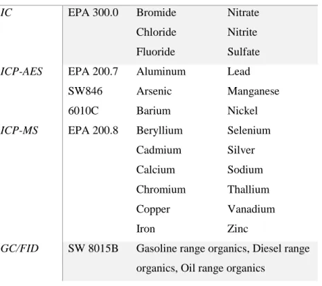
Table 1. Analytical methods used in this inter-laboratory comparison, along with the analytes chosen for analysis. Each laboratory performed the following analysis on four different samples, including pretreated produced water, raw produced water, pretreated fracturing flowback, and raw fracturing flowback.
Analysis Method Analytes
IC EPA 300.0 Bromide Chloride Fluoride Nitrate Nitrite Sulfate ICP-AES ICP-MS EPA 200.7 SW846 6010C EPA 200.8 Aluminum Arsenic Barium Beryllium Cadmium Calcium Chromium Copper Iron Lead Manganese Nickel Selenium Silver Sodium Thallium Vanadium Zinc
GC/FID SW 8015B Gasoline range organics, Diesel range organics, Oil range organics
2.3 Determination of inorganic anions by ion chromatography (IC): EPA method 300.0
Anions concentration was measured by IC using EPA Method 300.0. The EPA tested this method on a number of matrices, including drinking water and wastewaters [27]. IC is sensitive to water with high conductivity requiring filtration and dilution of the samples. Once prepared, this analysis requires introduction of a small volume of sample (roughly 2 mL) into an IC. The ions are subsequently separated and measured using a system comprised of a guard column, analytical column, suppressor device, and
9
conductivity detector. This method allows for modifications as long as they are fully documented and are consistent with quality control procedures, as outlined in Section 9.0 of the method.
When using EPA Method 300.0, a minimum quality control requirement includes initial determination of method detection limits (MDLs, found in Appendix B) and calculating a linear calibration range (LCR) as seen in Figure 1 [27].
Figure 1. The Linear Calibration Range (LCR) as calculated by New Mexico State University for this inter-laboratory comparison. The LCR must be verified every six months as required by EPA Method 300.0.
The results of this analysis may be affected by high concentrations of anions interfering with the peak resolution of adjacent anions. Additionally, substances with similar retention times, suspended materials greater than 0.45 microns, high concentrations of small organic anions, and presence of chlorine dioxide will cause interference in the results.
10
2.4 Determination of metals and trace elements in water and wastes by inductively coupled plasma – atomic emission spectrometry (ICP-AES): EPA Method 200.7 and SW 846 Method 6010C
Either EPA Method 200.7 or SW 846 Method 6010C was used to determine cations in an aqueous solution with ICP-AES. These methods have been verified for use in analyzing a number of matrices, including drinking water, industrial waste, and solid samples by the EPA, as described by the methods [28, 29]. The two methods are similar and give nearly identical results when applied to the same sample.
Samples are prepared in one of two ways that allows for analysis of either total recoverable analytes or dissolved analytes. In the current inter-laboratory comparison the analysis was used to characterize total recoverable analytes. The samples were prepared using EPA Method 3010. Once prepared, the samples were analyzed on a calibrated instrument following quality control as outlined in Sections 9.00 of method 200.7.
The quality control procedures require the determination of method detection limits, establishing MDLs (found in Appendix B), establishing the linear dynamic range (LDR), and verifying performance based on calibration standards [29].
In produced and flowback waters, interferences may be caused by high dissolved solids, and can be reduced through dilution of the sample. The laboratories participating in this inter-laboratory comparison diluted the samples between 30 and 100 fold.
2.5 Determination of trace elements in waters and wastes by inductively coupled plasma – mass spectrometry (ICP-MS): EPA Method 200.8
Depending on the capability of the laboratory, cations were also analyzed using EPA Method 200.8. This method utilizes ICP-MS to determine cations in a number of matrices. Like EPA 300.0, EPA 200.7, and SW 846 6010C, this method underwent an inter-laboratory collaborative study to determine the applicability to different matrices, including ground and surface water, municipal primary effluent, industrial wastewaters, and soils [30]. The samples were prepared using either EPA Method 3010, or an in
11
house method that included microwave digestion at 180 °C, and the use of hydrogen peroxide in addition to nitric and hydrochloric acids to aid the digestion of the high organic content samples.
In the current inter-laboratory comparison, samples analyzed using this method were prepared by the same methods mentioned in Section 2.4 above to analyze total recoverable analytes. Interferences of abundance sensitivity may be an issue with produced and flowback water as many analytes are found in extremely high concentrations, including calcium and chloride.
2.6 Nonhalogenated organics using gas chromatography/flame ionization detector (GC-FID):
SW 8015B
GRO, DRO, and ORO were characterized using SW 846 Method 8015B. This method determines the volatile and semivolatile organic compounds with GC-FID. GRO characterization gives a concentration of alkanes from C6 to C10 that have a boiling point between 60 and 170 ºC. GRO are extracted from aqueous solutions before injection into the GC-FID by multiple techniques including purge-and-trap, automated headspace recovery, and vacuum distillation, depending on the laboratory’s capability. DRO characterization gives a concentration of alkanes from C10 to C28 that have a boiling point between 170 and 430 ºC. DROs are extracted from aqueous solutions before injection to the GC-FID using solvent (liquid-liquid) extraction. ORO is an extended calibration of DRO, and this characterization gives a concentration of alkanes from C20 to C35. Samples are prepared using SW 846 Method 3010 C. This method is used because currently there is no total petroleum hydrocarbon method approved by the EPA. An alternate method available is n-hexanes extraction of total oil and grease (EPA method 1664A). Method 1664A is known to overestimate total petroleum hydrocarbons because it samples more water-soluble compounds including carboxylic acid in addition to the petroleum hydrocarbons [31]. However, this method does not provide a characterization of the petroleum carbon profile as SW 846 Method 8015B does. As McFarlane discusses, effective remediation of oil and gas production and development water depends on an accurate profile of the types and amounts of hydrocarbons in the wastewater [31]. A carbon profile, both
12
before and after treatment, will show how the petroleum hydrocarbons change after oxidation, coagulation, and filtration.
The extended calibration used for DRO/ORO analysis was conducted by altering the temperature program from what was called for in the original SW 846 Method 8015B. The program may be different depending on the labs. To demonstrate this, two GC conditions and temperature programs from two labs included in this comparison, Accutest and CUB, are included below. The GC conditions and temperature program used at CUB were as follows:
Column: Restek Rxi-1ms, 0.18 mm ID, 20 m length, 0.18 µm film thickness
Volume injected: 4 µL
Constant carrier gas (helium) pressure: 14.5 psi
Split flow: 50 ml/min
Injector temperature: 275 °C
Detector temperature: 350 °C
Temperature program: 40 °C, held for 1 minute, increased at 20 °C/min to 330 °C and held for 20 minutes.
Standard: C8—C40 Alkanes
The GC conditions and temperature program used at Accutest were as follows:
Column: Restek RTx-5, 0.53 mm ID, 30 m length, 1.5 µm film thickness
Carrier gas (helium) flow rate: 5-7 mL/min
Makeup gas (helium) flow rate: 30 ml/min
Injector temperature: 200 °C
Detector temperature: 340 °C
Temperature program: 75 °C for 3 minutes, 15 °C/min to 300 °C for 4 minutes, 20 °C/min to 330 °C for 9 minutes
13
Standards: Diesel Fuel #2 and SAE 30W Motor Oil
The GC-FID is a sensitive instrument and many complications arise when testing oil and gas development and production wastewater samples. One such complication when testing samples that contain heavy hydrocarbons is retention of the hydrocarbons in the column and bleed in the chromatogram in subsequent samples.
2.7 Quality assurance
To ensure the quality of the data produced, each laboratory followed and reported the quality assurance/quality control (QA/QC) practices that were followed in the handling, preparation, and analysis of the samples. These practices included recording how the samples were handled upon arrival and prepped for analysis. Calibration procedures for their equipment was also recorded, including recent calibration dates both before and after the samples were analyzed, the calibration range used for analyzing the samples, the deviation between calibration curves, and the allowable deviation from the calibration curve. Finally, duplicate analysis was requested for each of the analyses.
Once the participating laboratories reported their analytical results, the data were analyzed for outliers using the Grubb’s test with both 0.05 and 0.001 significance level following the protocol outlined by Feinberg (1995) and Hund et al. (2000) [32, 33]. The outliers at 0.05 significance level were noted as stragglers, but left in the data. The outliers at 0.01 significance level were taken out of the data. Once the initial round of outliers were removed, that data was once again subjected to the Grubb’s test, and any additional outliers that were found were either rejected or left in the dataset depending on the significance level of which they were outliers, as discussed above. Analytes that generated two outliers are considered to be variable [33]. Additionally, analytes that were reported as below detection limit or below reporting limit were also not included in the results. Further statistical evaluation was carried out using Microcal Origin 6.0, giving the mean, standard deviation, median, first and third quartile, and box and whisker plots were generated. Once the mean was calculated with the corrected data, the relative standard deviation
14
(RSD) was calculated and compared to the mean, standard deviation, and RSD were compared to those reported by the EPA comparative inter-laboratory comparisons for the respective method and analyte. Other aspects of this study were compared between participating laboratories, including detection/reporting limits. These tables are found in Appendix B along with tables of the mean, standard deviation, and range.
15
CHAPTER 3 RESULTS AND DISCUSSION
The results from the inter-laboratory comparison are found below. The results are separated into performance by anion, performance by cation, and total petroleum hydrocarbons.
3.1 Performance by anion
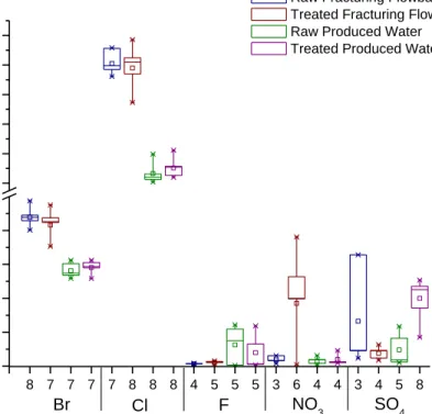
Anions analyzed by EPA 300.0 were found in all matrices, both raw and treated produced water and fracturing flowback wastewater. The results for the analyzed anions are shown in Figure 2. In some cases there was an increase in concentration between the raw and treated samples, as seen in the concentration of bromide and sulfate in treated and raw produced water samples and nitrate in the treated and raw flowback water. Chloride concentration was expected to increase in the treated samples because aluminum chloride was used as a coagulant; however, this was not seen with both of the treated wastewater samples. The mean chloride concentration in the treated fracturing flowback water slightly decreased while slightly increasing in the treated produced water.
Outliers were not common in the reported anion results. Bromide analysis from one laboratory was consistently an outlier at 0.01 significance level, and removed from the data analysis. The only other outlier determined was one fluoride datum at 0.05 significance level. This was left in the dataset as described in Section 0.
The reported concentrations for many of the anions seemed to be bimodal in nature. For example sulfate displayed this trend in the raw fracturing flowback, treated fracturing flowback, and raw produced water. Specifically, the treated fracturing flowback dataset for sulfate consisted of four concentrations, 3.45 mg/L, 4.79 mg/L, 9.21 mg/L, and 12.65 mg/L. There were no outliers taken out in this data because the mean reflected both the high and low concentrations reported. However, from this dataset, it is extremely difficult to ascertain a correct concentration. The data are not weighted in one direction or another. This trend is again displayed in the raw produced water data, with reported concentrations from five different participating laboratories of 2.08 mg/L, 2.44 mg/L, 3.66 mg/L, 16.49 mg/L, and 23.40 mg/L. These data distribution does not give an accurate characterization of the water over multiple laboratories because there
16
is not a way to validate which of these concentrations is correct. These bimodal data are also displayed by fluoride concentrations in raw produced water and nitrate in all four water samples.
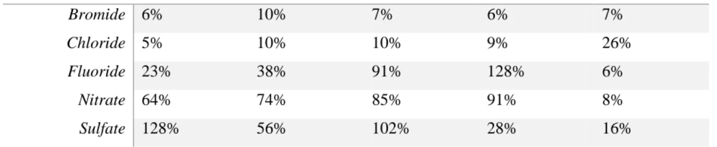
Variation within populations was measured by the RSD. Those with the greatest RSD were fluoride, nitrate, and sulfate, all with values greater than 60%, with the exception of fluoride in both the raw and treated fracturing flowback samples (23% and 38%) and sulfate in the treated produced water (28%). Bromide and chloride showed the least variation with RSD values, at or below 10%. Nitrite was not considered for further statistical analysis because only one laboratory reported detectible concentrations.
Although the anions did not have many outliers in the data, the RSD for the three anions of lesser relative concentrations (i.e., fluoride, nitrate, and sulfate) were all relatively high (greater than 60%). This variability may result from different factors, with the most noticeable being interference from the surrounding matrix. One such example is fluoride. Fluoride is often variable due to interference from the adjacent chloride peak [34]. As Prusisz et al. discuss, high concentrations of chloride overwhelm the column, causing either distortion or complete masking of the fluoride peak [34]. This phenomena may be exacerbated by anions that are in high concentrations, requiring dilution and resulting in non-detection of the anions that are now at a concentration low enough that the analytical instrument has difficulty detecting them. This may have caused the almost complete non-detection of nitrite. The nitrate peak is also substantially affected by the tail end of the chloride peak, obscuring the nitrate peak at high chloride concentrations [35].
Anions at higher concentrations (i.e., bromide and chloride) did not vary as significantly as those at lower concentrations. One bromide datum was removed per dataset for each matrix analyzed, encouraging a more uniform distribution of the remaining data, and resulting in a lower RSD. The outlier removed for bromide was consistently from one laboratory, and therefore might have resulted from calibration error rather than variation in the analysis. Chloride was the most abundant anion in solution for all four water samples, making it easier to determine an accurate concentration over multiple trials and across multiple laboratories.
17
Table 2. Summary of RSD values for the anions that displayed the highest variability in analysis compared to the RSD values as reported by EPA Method 300.0. The matrices are raw fracturing fluid (RFF), treated fracturing flowback (TFF), raw produced water (RPW), and treated produced water (TPW). RFF TFF RPW TPW EPA 300.0 Bromide 6% 10% 7% 6% 7% Chloride 5% 10% 10% 9% 26% Fluoride 23% 38% 91% 128% 6% Nitrate 64% 74% 85% 91% 8% Sulfate 128% 56% 102% 28% 16%
When the EPA validated this method, an inter-laboratory comparison (n=19) was performed for all anions that are analyzed with this method in three different matrices, including reagent water, drinking water, and wastewater [27]. In most cases, the standard deviation reported in the EPA inter-laboratory comparison was significantly less than the standard deviation resulting from the analysis of oil and gas wastewater for similar concentrations. For example, the standard deviation for fluoride at concentrations of 6.79 mg/L and 8.49 mg/L in the EPA analysis of wastewater had a standard deviation of 0.41 and 0.36, respectively [27]. The standard deviation for fluoride in the treated produced water was 10.22 with a mean of 7.96 mg/L. However, it is difficult to compare the anions tested in the EPA inter-laboratory comparison to this analysis because the range of concentrations are different. For example, the highest chloride concentration tested by the EPA was 26.0 mg/L, with a reported standard deviation of 2.50 for wastewater and 2.65 for drinking water. The concentration of chloride analyzed in the oil and gas wastewater was between 7,028 mg/L and 14,094 mg/L, with standard deviations ranging from 598 mg/L to 1,426 mg/L. The samples were diluted prior to analysis, but even at 100x dilution, the concentrations analyzed in the oil and gas wastewater are 3.5 to 7 times greater than what was analyzed by the EPA study.
However, with matrices as complex as what is found in oil and gas wastewaters, what is being lost in preparation and analysis must also be considered. The samples were diluted by the participating laboratories between 30 and 100 fold. Due to this dilution, many anions were reported as “below detection limit” or “below reporting limit.” For example, fluoride, nitrate, nitrite, and sulfate were not detected in
18
50% of the results on average. Nitrate and nitrite is found in very low concentrations in the oil and gas wastewaters used in this study and therefore dilution would greatly affect the detection of these anions.
The variability observed in the results most likely arises from the unique oil and gas wastewater matrix. The high chloride concentrations that are found in in the majority of produced and flowback waters complicates the analysis of surround anions. Fluoride, nitrite, nitrate, and bromide are heavily influenced by chloride interference and peak overlapping, making accurate interpretation of the chromatogram difficult [34, 36]. According to Novič et al., increased retention times for nitrate and nitrite were seen in matrices with high chloride concentrations. The mechanisms driving this elution are twofold. As the sample plug moved through the column, the chloride ions prevent retention of both nitrate and nitrite in the stationary phase [36]. However, there was an overall increase in retention time caused by an on-column change in the eluent [36]. Therefore, the reported size, shape, and retention time of the nitrate and nitrite peaks change in the presence of chloride.
Figure 2. Five anions analyzed in the four oil and gas wastewater streams. The horizontal tick labels represent the number of results that were reported as detectable concentration for the anion. Aluminum chloride was used as a coagulant, slightly increasing chloride levels in the treated produced samples.
8 7 7 7 7 8 8 8 4 5 5 5 3 6 4 4 3 4 5 8 0 20 40 60 80 6000 8000 10000 12000 14000 16000 Anion SO 4 NO 3 F Cl Br C o n ce n tr a ti o n ( m g /L )
Raw Fracturing Flowback Treated Fracturing Flowback Raw Produced Water Treated Produced Water
19
Another source of significant interference can arise from carbonates present in the samples. The alkalinity of produced water is reported to be between 54.9 and 9,450 mg/L as CaCO3 in the literature, with the majority having more than 200 mg/L as CaCO3 [8, 37]. The samples were analyzed for alkalinity at CSM using the Hach test for alkalinity and were found to be 620 mg/L as CaCO3 for the raw fracturing flowback, 330 mg/L as CaCO3 for the treated fracturing flowback, 650 mg/L as CaCO3 for the raw produced water, and 600 mg/L as CaCO3 for the treated produced water. High concentrations of carbonate and dissolved CO2 increase the peak width and decrease the height of the chloride peak, and changed the retention times of chloride, bromide, and sulfate irreproducibly, making analysis variable [38]. Due to the matrix interference, Novič et al. suggest that IC should not be used on complex matrices because the results are variable [38]. Overall, the variability is most likely a complex interaction of a number of compounds that are naturally found in oil and gas wastewater samples.
3.2 Performance by cation
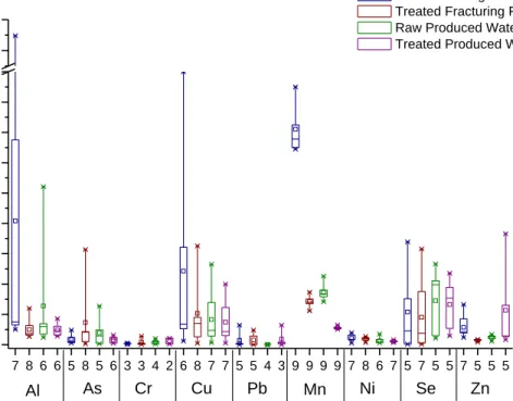
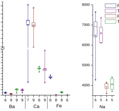
Cations analyzed by EPA 200.7 and 200.8 or SW 846 6010C were found in all four matrices; although, many of the trace cations were not reported by enough laboratories to be included in statistical analysis. The results for the cation analysis are summarized in Figures 3 and 4. There are nine data points for some of the cations analyzed because Accutest performed SW 846 Method 6010C as well as 200.7 and 200.8 for the characterization of the wastewater samples. The data from SW 846 Method 6010C was included in the statistical analysis as a separated data set rather than a replicate analysis because the calibration and date of analysis were different. The cations are divided into two graphs by concentration, with those having a reported concentration less than 2 mg/L being shown in Figure 3, and those with a reported concentration greater than 2 mg/L shown in Figure 4. With the exception of zinc in the produced water and arsenic in the flowback, almost all cations decreased in concentration after treatment. Those that decreased most significantly were aluminum, manganese, and copper.
20
Outliers were removed as described in Section 0. The data were tested multiple times for outliers. Up to two outliers were removed if they were found to be outliers at the 0.01 significance level with the Grubb’s test. The outliers at the 0.05 significance level were left in the dataset, but were noted. The matrix that had the most outliers was the raw produced water (10 outliers at the 0.01 significance level, and two at the 0.05 significance level), followed by treated produced water (five outliers at the 0.01 significance level and two outliers at the 0.05 significance level). The treated fracturing flowback data contained seven outliers at the 0.01 significance level and two at the 0.05 significance level and the raw fracturing flowback data contained five outliers at the 0.01 significance level and three at the 0.05 significance level. The analytes that consistently had the most outliers in all matrices were aluminum, arsenic, barium, chromium, iron, lead, and zinc. The high occurrence of outliers in the data suggests that the analysis is very variable [33].
Figure 3. Cations found in oil and gas development and production wastewaters, both before and after treatment. The horizontal tick labels represent the number of results reported as a detectable concentration of the cation. 7 8 6 6 5 8 5 6 3 3 4 2 6 8 7 7 5 5 4 3 9 9 9 9 7 8 6 7 5 7 5 5 7 5 5 5 0.0 0.2 0.4 0.6 0.8 1.0 1.2 1.4 1.6 1.8 3.6 3.8 Cation
Raw Fracturing Flowback Treated Fracturing Flowback Raw Produced Water Treated Produced Water
Zn Se Ni Mn Pb Cu Cr As Al C o n c e n tr a ti o n ( m g /L )
21
The cations that were removed from further statistical analysis were beryllium, cadmium, thallium, silver, and vanadium due to the large number of laboratories that reported non-detection. In most cases, two laboratories reported detectable limits for these cations, with the exception of beryllium, with only one laboratory reporting a detectable concentration. The anions that were reported by four or more laboratories for one of the matrices were included in all subsequent statistical analysis.
The pattern of bimodal data was also found in some of the cation results. Those that displayed this characteristic were aluminum, arsenic, chromium, copper, selenium, and zinc. This data distribution is most common in the raw fracturing flowback. The variation may be due to the higher levels of chloride and calcium causing interference in the analysis.
Figure 4. Analytical results for the major cations found in both the treated and untreated oil and gas development and production wastewaters. The horizontal tick labels represent the number of analytical results available for the cations.
6 9 9 9 7 9 8 9 6 8 8 6 0 20 40 60 80 100 120 140 160 400 600 800 1000 1200 1400 Cation Fe Ca Ba C o n c e n tr a io n ( m g /L ) 6 5 4 5 4000 5000 6000 7000 8000 Na
Raw Fracturing Flowback Treated Fracturing Flowback Raw Produced Water Treated Produced Water
22
The majority of the cations analyzed were found to be either moderately (RSD between 10% and 60%), or significantly (RSD greater than 60%) variable between labs. Aluminum, arsenic, chromium, copper, lead, nickel, selenium, and zinc had RSD values above 60%, with few exceptions, including aluminum in treated produced water (RSD of 46%) and zinc in both the treated fracturing flowback and raw produced water (RSD of 28% and 36%, respectively). Those with the greatest variation as defined by a high RSD value for all four matrices were copper (RSD between 97% and 132%) and lead (RSD between 80% and 195%). The analysis of iron was variable between matrices, with RSD value fluctuating from 6% to 20% in the raw flowback and treated flowback samples, respectively; however, the RSD rises from 11 to 110% between the raw produced and treated produced samples. Those that have less variability were manganese, barium, calcium, and sodium; however, their RSD values still fluctuate between matrices with some above 10%. The least variable was sodium, with RSD values of 20%, 8%, 6%, and 8% for the raw flowback, treated flowback, raw produced, and treated produced water, respectively. Barium had RSD values that slightly decreased with treatment, with 14% and 25% RSD for the raw fracturing and produced water, decreasing to 13% and 22% with pretreatment. The RSD for calcium decreased from 42% to 27% with treatment in the fracturing flowback water, but increased from 7 to 31% with treatment in the produced water.
Unlike the anions, many of the cations that were found at lower concentrations were not only variable when considering the RSD, but the data also contained more outliers. The RSD values for the cations that displayed the most variability in analysis are found in Table 3, along with the RSD values from the EPA method validation data. Those that were the least variable were the cations that were found in the highest concentrations in the four samples, calcium, and sodium (Figure 4). The outliers did not result from only one or two labs, but varied between lab, water sample, and analyte. Additionally, as discussed above, the RSD for nearly all analytes with a concentration below 2 mg/L are highly variable (RSD above 60%). Like the anions, this may result from a number of factors, including matrix interference caused by high levels of chloride and calcium.
23
The EPA performed an inter-laboratory comparison to validate Method 200.7 for multiple matrices [29, 30]. For EPA’s industrial effluent analysis, the wastewater contained trace concentrations of most analytes. The matrix was then spiked to a low and high concentration. For example, aluminum was originally found at a concentration of 0.054 mg/L, and spiked to 0.05 mg/L and 0.2 mg/L [29]. The percent recovery and standard deviation of the percent recovery were then reported. For sliver, the standard deviation for the low spike was 0.585 mg/L, and for the high spike was 0.78 mg/L. For the oil and gas wastewaters, the mean concentration was between 0.816 mg/L and 0.096 mg/L, and the standard deviation was between 3.6 mg/L for the highest concentration and 0.12 mg/L for the lowest [29].
A similar inter-laboratory comparison was completed for Method 200.8 with 10 participating laboratories [30]. The concentrations in the study were between 100 and 350 µg/L [30]. The cations with the largest RSD were beryllium, aluminum, chromium, vanadium, and copper, with RSD values ranging from 10 to 16% [30]. The majority of the concentration ranges analyzed in the EPA method validation were similar to the concentrations found in this inter-laboratory characterization of oil and gas wastewater. However, the RSD values for the oil and gas wastewater analysis were between 45 and 151%. As both the sample size and the concentrations were similar for the EPA study as the analysis performed on the oil and gas wastewaters, this difference in RSD values speaks to the variability that occurs when the method is applied to this matrix.
The EPA performed an inter-laboratory comparison for SW 846 Method 6010C as well, with a maximum number of participants of eight [28]. All cations analyzed by this method had RSDs below 10%. Those that had the highest relative RSD were chromium, selenium, silver, thallium, and zinc, with RSDs between 8 and 10% [28]. RSD for the same analytes in the oil and gas wastewaters ranged from 28 to 151%. The concentrations analyzed were much higher in the SW 846 method than what was detected in the current oil and gas wastewaters, which may have resulted in a lower RSD. However, it is also likely that matrix interference caused the rise in variation as the concentrations analyzed were within the machine detection limit.
24
Table 3. Summary of RSD values for the cations that displayed the highest variability in analysis compared to the RSD values for the three methods used to analyze cations in this inter-laboratory comparison. The matrices are raw fracturing fluid (RFF), treated fracturing flowback (TFF), raw produced water (RPW), and treated produced water (TPW).
RFF TFF RPW TPW EPA 200.7 [29] EPA 200.8 [30] SW 6010C [28] Aluminum 16% 67% 151% 46% 12% 12% 6% Arsenic 96% 144% 122% 68% 3% 6% 6% Chromium 40% 151% 97% 114% 6% 8% Copper 13% 115% 111% 97% 23% 4% 6% Lead 19% 140% 80% 164% 20% 4% 6% Nickel 57% 34% 85% 32% 4% 8% 6% Selenium 13% 124% 77% 67% 3% 10% 8% Zinc 67% 28% 35% 131% 6% 18% 8% Barium 14% 13% 25% 22% 3% Calcium 42% 27% 7% 32% 7% Iron 6% 20% 11% 110% 6% Manganese 11% 12% 14% 8% 7% Sodium 20% 8% 6% 8% 4%
However, as previously mention, the oil and gas wastewater matrix is complex, and what is being lost in preparation and analysis must also be investigated. The samples were diluted by the participating laboratories between 5 and 100 fold. This dilution substantially limits sensitivity. Additionally, depending on the acid digestion method used prior to analysis, the reported concentration may be different. For example, two participating laboratories used digestion techniques that heated the samples to 180 °C, rather than 90 °C as indicated in EPA Method 3010A. One participating laboratory oxidized the organics with hydrogen peroxide in addition to nitric and hydrochloric acids. Any difference in reported concentration would be most prominent in the raw wastewater samples. However, there was not a significant rise in reported concentration between this laboratory and the other laboratories.
The variation in analytical results when characterization was performed with the ICP-MS may be both spectral and non-spectral in nature. Non-spectral interferences are induced by the sample matrix and
25
are often corrected for by internal standardization. However, correcting for matrix interference is impossible in certain situations, specifically, correcting for interference in a matrix that contains a large number of elements is difficult [39]. Additional non-spectral interference may come from organic matter and polyatomic interference. Goossens et al. report that small concentrations of organic matter in the samples can enhance signals but also shift the maximum signal intensity to lower gas flow-rates [39]. This interference significantly affects arsenic and selenium signals in a way that cannot be easily corrected for by internal standardization [39]. This interference is exacerbated by a chlorine matrix causing polyatomic interferences [39]. Polyatomic interferences, such as that cased by chloride, are the cause of most non-spectral interferences in ICP-MS [40]. Additionally, easily ionizable elements (i.e. sodium, magnesium, and potassium) that are in the sample solution can cause non-spectral interferences and variability in the results [41].
Non-spatial interference occurs in ICP-AES as well as ICP-MS. The effect of easily ionizable elements such as sodium and calcium can induce changes in the signals of the other elements being analyzed [41-45]. These easily ionizable elements create significant background enhancements when they are found at high concentrations. Additionally, this phenomena seems to cumulative. A matrix that has many easily ionizable elements combined in solution is more variable due to an increase in the true detection limit of the ICP-AES This effect has been investigated on the analytical results for aluminum, calcium, chromium, cadmium, and zinc [44, 46]. The matrix effect caused by sodium can be reduced or eliminated through robust plasma operating conditions [47]. However, the use of a robust plasma operating condition only moderately lessens the matrix effect elicited by calcium [44, 47]. Furthermore, Ghazi et al. report that a complex matrix can also raise the RSD of the results, due to overlap of analysis lines of analytes [44].
Therefore, the variability observed in the analysis of oil and gas development and production wastewaters is a complex interaction of the complexity of the matrix, and the presence of ions that are known to create matrix induced interference. This problem is compounded by both the concentration and number of easily ionizable elements in solution. It would be difficult to compensate for all the causes of non-spatial variance in oil and gas wastewaters. Although, the samples were oxidized to remove organic
26
matter prior to analysis, it is unknown if any organic matter could remain in the samples. Additionally, the sensitivity of the ICP is highly effected by the easily ionizable elements, giving greater variation in results. Therefore, the results may not be a true representation of the actual concentration of the elements analyzed.
3.3 Total Petroleum Hydrocarbons
Petroleum hydrocarbons were analyzed as described in Section 0. The analysis of the oil and gas wastewaters were performed in two batches, the first was performed by the two commercial laboratories that received the raw and treated, un-extracted samples. unextracted. The second was performed by the University of Colorado, Boulder (CUB) with samples extracted by Accutest Environmental Testing Laboratory. The sample analysis at CUB were performed in duplicate with the method blanks, method spikes, and method spike duplicates. The concentrations reported by each of the labs participating in the DRO and ORO analysis are summarized in Table 2. The combination of DRO and ORO are also termed extractable petroleum hydrocarbons (EPH). Although three months separated the commercial laboratory EPH analysis from the analysis performed at CUB, the hydrocarbon concentrations reported by CUBCU were very similar to those reported by Accutest and Stewart Environmental (Table 4). The chromatograms from CUB are included in the discussion because they better display the changes in the carbon profile when oil and gas wastewaters are treated with ozonation.
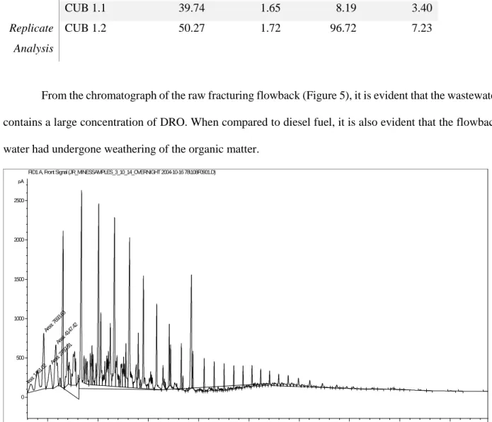
When the raw fracturing flowback was ozonated, the concentration of EPH decreased significantly, from an average of 51 mg/L to 3 mg/L. When the chromatogram of the raw fracturing flowback (Figure 5) is compared to the chromatogram of the treated fracturing flowback (Figure 6), it is demonstrated that the majority of oil and gas range organics are oxidized; however, one peak remains in the treated fracturing flowback that corresponds to a C20 alkane. When the raw produced water was ozonated, the average concentration decreased from 7.6 mg/L to 4.4 mg/L. When the raw produced water chromatogram (Figure 7) is compared to the treated produced water chromatogram (Figure 8), results imply that the treatment is not as effective, with some large peaks remaining after treatment corresponding with C14 and C20 alkanes. The C14 alkane may be tetradecane, and the C20 alkane may be icosane.
27
Table 4. Summary of GC/FID results for combined diesel and oil range organic concentrations (mg/L) from participating laboratories for raw fracturing flowback (RFF), treated fracturing flowback TFF), raw produced water (RPW), and treated produced water (TPW). The missing cells represent analysis that were unsuccessful due to inadequate volume. The laboratories that reported EPH concentrations were Accutest (ACC), Stewart Environmental (SE), and University of Colorado, Boulder (CUB). CUB n.1 is the first round of analysis, with the n representing the replicate number, and CUB n.2 is the second round of analysis.
Participating Laboratory RFF (mg/L) TFF (mg/L) RPW (mg/L) TPW (mg/L) ACC 76.40 2.07 11.58 4.32 SE 40.00 < 5.00 < 5.00 < 5.00 CUB 1.1 39.74 1.65 8.19 3.40 Replicate Analysis CUB 1.2 50.27 1.72 96.72 7.23
From the chromatograph of the raw fracturing flowback (Figure 5), it is evident that the wastewater contains a large concentration of DRO. When compared to diesel fuel, it is also evident that the flowback water had undergone weathering of the organic matter.
Figure 5. Chromatogram of the raw fracturing flowback extraction. The DRO elute between 5.53 and 14.18 minutes. The ORO elute between 14.18 and 23.20 minutes. The majority of the organics found in raw fracturing flowback are between C8 and C33.
min 5 7.5 10 12.5 15 17.5 20 22.5 25 pA 0 500 1000 1500 2000 2500
FID1 A, Front Signal (JR_MINESSAMPLES_3_10_14_OVERNIGHT 2004-10-16 78\108F0901.D)
Are a: 14 61.02 Are a: 76 93.63 Are a: 27 97.91 Are a: 41 47.42
28
It is difficult to make a comparison to the results reported for aqueous samples in the EPA method as was done for the previous comparisons between the analyses completed in this inter-laboratory comparison to the inter-laboratory comparison performed by the EPA with domestic wastewater for the approved method. The extraction method chosen by the EPA for aqueous samples was different than the method used in this study. However, the second matrix studied by the EPA was sandy loam soil spiked with diesel fuel, extracted with methylene chloride [48]. In order to disregard any difference that may come from a comparison between solid-liquid extraction and liquid-liquid extraction, the percent difference between the spiked concentration and the reported analyzed concentration was not compared, only the standard deviation and RSD are be considered. The EPA study is similar to what was performed in this comparison because the EPA analyzed five replicates in order to calculate the mean and standard deviation for each concentration analyzed. This study has six replicates from one laboratory that can be averaged, and two other labs that analyzed the oil and gas wastewater samples months before.
Figure 6. Chromatogram of the treated fracturing flowback extraction. The DRO elute between 5.53 and 14.18 minutes. The ORO elute between 14.18 and 23.20 minutes. The majority of the organics found in treated fracturing flowback are between C8 and C20, with the only substantial peak being C20.
min 4 6 8 10 12 14 16 pA 0 200 400 600 800 1000 1200 1400 1600
29
Figure 7. Chromatogram of the raw produced water extraction. The DRO elute between 5.53 and 14.18 minutes. The ORO elute between 14.18 and 23.20 minutes. The majority of the organics found in raw produced water are between C8 and C20, with the only substantial peak being C20.
The EPA analysis was performed twice with the same matrix. The first included five different spiked diesel concentrations: 12.5 mg/L, 75 mg/L, 105 mg/L, 150 mg/L, and 1000 mg/L [48].The second included four different spiked concentrations 25 mg/L, 75 mg/L, 125 mg/L and 150 mg/L [48]. The mean concentration reported for the first analysis of 75 mg/L was 54 mg/L, with a standard deviation of 7 mg/L [48]. The second analysis of 75 mg/L reported a mean concentration of 75.9 mg/L with a standard deviation of 7.8 mg/L [48]. The RSD was calculated to be 13% for the first analysis, and 10% for the second. For the oil and gas wastewater samples analyzed by CUB, the average concentration of EPH for the raw fracturing flowback (the sample with the greatest concentration) was 44.4 mg/L with a standard deviation of 8 mg/L and RSD of 18%. The average for the two commercial labs was 58.2 mg/L with a standard deviation of 18.2 mg/L and RSD of 31%. When the standard deviation of this study is compared to the EPA’s study, the RSD for the analysis of oil and gas wastewaters is greater than those found by the EPA. The RSD of the commercial labs was greater than RSD for CUB. This is easily explained by the analysis being completed by one lab versus two. There is a greater possibility that the differences between laboratories is greater than
min 4 6 8 10 12 14 16 18 20 22 pA -250 0 250 500 750 1000 1250 1500 1750
30
within one laboratory. The raw produced water samples CUB 2.2 and 2.3 are a severe outlier of the data that may come from contamination of the column, or some other calibration failure because they are so dissimilar to the other concentrations reported for the raw produced water samples.
Figure 8. Chromatogram of the treated produced water extraction. The DRO elute between 5.53 and 14.18 minutes. The ORO elute between 14.18 and 23.20 minutes. The majority of the organics found in treated produced water are between C8 and– C20, with the only substantial peak being C20. After treatment, many diesel range organics remain in the produced water.
The Massachusetts Department of Environmental Protection published a method very similar to the EPA Method 8015B, called the Method for the determination of extractable petroleum hydrocarbons [49]. This method includes more information regarding EPH concentration calculation, and has very thorough directions for characterizing EPH. This method also includes the mean, standard deviation, and RSD for each alkane that can be analyzed with this method. The RSD ranged from 0.7% for C10 to 17.5% for C16 at a concentration of 2.5 µg/L for each alkane for each of the seven replicates [49].
Therefore, the RSD reported in the Method for the determination of extractable petroleum hydrocarbons is lower than the RSD for the current inter-laboratory analysis. However, due to the small
min 5 7.5 10 12.5 15 17.5 20 22.5 pA -250 0 250 500 750 1000 1250 1500 1750
31
sample size, this analysis needs to be replicated with a larger sample size to see if the RSD remains high when more laboratories are included.
The data in Table 2 demonstrates the difference in EPH concentration between laboratories. For example, the raw fracturing flowback EPH concentration was reported to be 76.40 mg/L by Accutest, and 40 mg/L by Stewart Environmental. The EPH concentration reported by CUB is similar to Stewart Environmental for the raw fracturing flowback, reporting an average of 43.95 ± 7.42 mg/L. However, the concentrations for the treated produced water is similar for all laboratories. No one laboratory reports relatively higher EPH concentrations than the others.
The GRO were tested by only two laboratories, Accutest and Stewart Environmental. The results of the GRO analysis are summarized in Table 5. The results for GRO in the raw fracturing flowback display a similar pattern to the EPH. Accutest reported a GRO concentration around four times greater than the concentration reported from Stewart Environmental for the raw fracturing flowback sample, 37.5 mg/L compared to 9 mg/L.
This variability may result from a number of sources. One of which being the solute/solvent relationship may be altered by matrix interferences, decreasing the effectiveness of the liquid-liquid extraction [31]. Another difference may be the standard chosen for calibration. CUB and Stewart Environmental used an EPH standard while Accutest used separate standards for DRO and ORO. The DRO and ORO results from Accutest were summed to find the concentration of EPH. Also, the standards used for all laboratories were unweathered while the samples analyzed were highly weathered. Heavily weathered diesel develops a larger envelope while experiencing evaporative losses of the lighter hydrocarbons. Therefore, the unweathered standards may not give a completely accurate analysis of the true EPH concentration. There is not a uniform significant difference between the different temperature program and column use.
32
Table 5. GRO concentration in mg/L as analyzed by Accutest (ACC) and Stewart Environmental (SE) for the raw fracturing flowback (RFF), treated fracturing flowback (TFF), raw produced water (RPW), and treated produced water (TPW).
RFF(mg/L) TFF (mg/L) RPW (mg/L) TPW (mg/L)
ACC 37.5 0.753 2.83 0.219