automated sequential composition of deltas and related optimization operations

(1)

September 2009

automated sequential composition of deltas

and related optimization operations

An additional research to metamodel independent difference representation

Bachelor Thesis

Universität Paderborn Matthias Heicke

Institut für Informatik Paderborn, Germany

Warburger Straße 100 it@heicke.de

33098 Paderborn, Germany Examiner: Prof. Wilhelm Schäfer, UPB

(+49) 5251 – 603313 Supervisor: Prof. Ivica Crnkovic, MDH

Mälardalen University

Division of Software Engineering Box 883, 721 23 Västerås, Sweden (+46) 21 – 101453 www.mdh.se/idt

(2)

2 Table of Contents

3.2.1 Difference Metametamodel (MMD) ... 17 3.2.2 Constructing Constraints/Rules... 18 3.2.3 Example ... 19 3.3 Difference Application... 20 3.4 Operators ... 21 3.4.1 Dual Calculation... 22 3.4.2 Sequential Calculation... 22 3.4.3 Parallel Calculation... 23 4 Sequential Calculation... 24 4.1 Concept ... 24 4.1.1 Constraints ... 25 4.2 Cases... 26 4.2.1 Existing ... 26 4.2.2 Non Existing... 27 4.2.3 Examples... 27 4.3 Implementation... 29

4.3.1 First Problem: adding or deleting of contained elements ... 29

4.3.2 Second Problem: changing an contained element ... 31

4.3.3 Testing ... 31

5 Personal Conclusion ... 33

5.1 Changing the Problem... 33

5.2 Future Work ... 35

Acronyms... 36

(3)

1 Introduction 3

“A grand challenge is to establish modelling as the basis of informatics.” [prof. Robin Milner]

1 Introduction

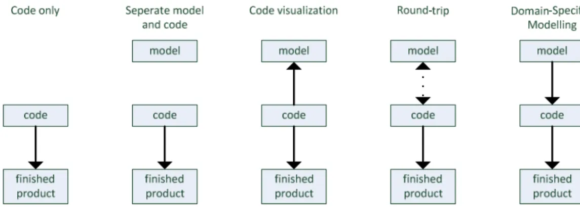
Since programmable computers became common, developers tried to raise the level of abstraction, making it easier to develop software on the one hand and avoiding errors in the developing phase on the other hand. This evolution of software engineering underwent several main steps, like the change from machine code to Assembler (2nd level programming language) to high level programming languages like FORTRAN or COBOL and later to PASCAL, C and Java. Model-Driven Engineering (MDE) was the next step in raising the abstraction. Combined with the concept of domain-specific modeling (DSM) it can increase productivity by 500-1000%, which happened last when there was a change from Assembler to high level languages. Today in use by companies like Nokia, it is still a rich area of research.1

To gain the most benefit of using models for software developing there’s a need for standardization. For software evolution purposes (and more) it is necessary, to not only handle models, but also the differences between them. In 2007 Antonio Cicchetti, Davide Di Ruscio, and Alfonso Pierantonio presented a metamodel independent approach to difference representation2. In the year 2008 Antonio Cicchetti presented his doctor thesis3, another paper with rich research on this topic. A sub theme of this paper is the sequential composition of those differences. This thesis presents an approach to sequential calculation, hence it can be considered as an enhancement/enlargement to Cicchettis work. According to this, these two papers are normally not mentioned as references in the text. References to other papers are done either by square brackets (e.g. [1]) or by superscription (e.g. 1). All other numerical references refer to chapters in this text.

1.1 Outline of the Thesis

The thesis starts with a broad overview of basic concepts, like Model-Driven Engineering (MDE), Transformations or Software Evolution. One focus is on ATLAS Transformation Language (ATL), the language later used to implement this approach. The second chapter of the thesis is about Differences with Cicchettis Meta-Model Independent Approach as the main focus. Also Operators are introduced, including Sequential Calculation, which is the next chapter. Once again, the Concept is explained and some Constraints are described, which need to be considered. Afterwards, the possible sequential calculations are divided into Cases and an Implementation approach is presented. Finally the Personal Conclusion of the author is presented, including an approach to solve several problems which occurred through the implementation research and a brief foresight on this topic.

(4)

4 2 Basic Concepts and Tools

2 Basic Concepts and Tools

In this chapter some of the basic concepts used by this thesis are outlined to inform readers who have no or only little contact to Model-Driven Engineering.

In section 2.1 the whole concept of software modeling (MDE, DSM) and the techniques used (MOF, KM3) are described. Section 2.2 introduces the concept of model transforming and

ATL, the transformation language which is used in this thesis. Section 2.3 is about model weaving. Finally in section 2.4 the concept of software evolution is introduced.

2.1 Model-Driven Engineering (MDE)

In traditional code-driven software engineering, models where often not anything more then personal drawings, desultory done for their own purpose by some developers, confined to a simple documentation role instead of being actively integrated into the engineering process1. Since models were always a vehicle for communication, they became rapidly an effective way to exchange all kind of information (design, interfaces, requirements etc) by all kind of developers (business process engineers, control engineers, computer scientists etc). MDE raises models into chief position of the designing phase in software engineering and so raises the abstraction grade of software designing.

In a first step models of the system and its components are designed to ease the communication, but also to provide an additional basis for pre-implementation, validation of requirements and quality properties as well as for automatic generation of source code4. In a second step the code is written manually, based on the constructed models (maybe supported by some automatisms).

The idea behind MDE is to find an easy, clean and productive solution for the designing phase of software engineering which is abstracted from the complexity of the implementation. It also provides some techniques for formal design checks (e.g. HLPNs5) and eases the use of patterns since they are often model-based.

Bézivin declares in his paper [6] “everything is a model”. Compared to the old approach: “everything is an object” this means that all structures can be represent as models leveraging models into first class position in all kinds of development. Some advantages of this idea are highlighted in this paper.

2.1.1 Domain Specific Modeling (DSM)

After several years of model driven engineering the lack of a universal approach became obvious: General Purpose Languages were too broad. Automatic implementation based on the designed models was not possible (although there are some approaches based on UML profiles, called Excutable UML or xUML) and so the coding was done mostly manually. In the implementation phase modifications of the system only appeared in the code, because of high maintenance costs. Corresponding models were left unchanged, leading to not updated, invalid - and hence useless - models. The obvious benefit of this technique is very low compared to the costs.

In DSM a solution is created for a narrow field of application called a domain. According to Kelly and Tolvanen a domain can be defined as an area of interest to a particular

development effort. Domains can be a horizontal, technical domain, such as persistency, user interface, communication, or transactions, or a vertical, functional, business domain, such as telecommunication, banking, robot control, insurance, or retail 3/page3. DSM raises the level of

(5)

2.1.1 Domain Specific Modeling (DSM) 5

abstraction beyond current programming. The narrower a domain is, the more possibilities for automation we get, hence domains often consist of smaller sub domains.

A DSM consists of three parts:

• A domain-specific modeling language (DSL) • A domain-specific code generator

• A domain framework

The DSL is a special language, designed or adapted to characterize a domain. A DSL is a set of coordinated models. Each of those models specifies one of the following aspects12:

• Domain definition metamodel (DDMM): introduces the basic elements of a model (such as places, transitions and arcs in a PetriNet) and their relations.

• Concrete syntaxes: transformations, which map the DDMM onto a display surface metamodel (such as circles for places in the PetriNet example)

• Execution semantics: may also map the DDMM to another DSL with an execution semantic or even to a GPL (for example, mapping the firing rules of the PetriNet to Javecode)

The domain-specific generator generates – based on one ore more models constructed in the correlating DSL – code which runs on the correlated domain framework.

Since the coding is done by the code generator, it’s sufficient, if this part of the DSM is created by high skilled programming experts. Later on, the models, done in the DSL, can be produced by nearly anybody, which makes it easier for domain experts to develop the software. In DSM the main aspect of the engineering is located on the modeling and – in contrast to the former – stays on the model. Obvious a lot of advantages arise, for example:

• Lower costs – since we need only few high paid experts to construct the framework and the code generator

• Better Quality – since the models can be checked for errors automatically (for example based on OCL) and the coding is done automatically through code generators which are optimized by high skilled engineers.

• Higher Range of developers – DSM distinguishes two roles: those who create the DSM and those who use it. Mostly DSL are easier to handle, hence even developers with no knowledge in coding but maybe more experience in the domain can produce the software.

• Higher Productivity – in the long term the designing productivity increases but the largest benefit takes place in maintaining the software.

Since most companies are acting in small business segments, DSM is ideal for them. Of course, DSM is not the perfect solution for all companies and cases.

(6)

6 2.1.2 Model-Driven Architecture (MDA)

Figure 2.1: DSM compared to other approaches

2.1.2 Model-Driven Architecture (MDA)

In 1996 the OMG started to expand their scope to modeling. Belonging development processes based on abstractions have been standardized and proposed by OMG under the name of MDA. Its main target is to separate the specification functionality from the specification of the implementation to solve the three primary goals which are portability, interoperability and reusability through architectural separation of concerns7. This is done in three steps. First of all, a Computation Independent Model (CIM) is constructed. This is later transferred to a Platform Independent Model (PIM) which already uses a general-purpose, platform independent modeling language such as UML. Finally this model is transferred into a Platform Specific Model (PSM), which focuses on the implementation details of a certain platform.8

MDA promises many benefits namely reduced costs throughout the application life-cycle; reduced development time for new applications; increased return on technology investments (ROI) and rapid inclusion of emerging technology benefits into existing systems.9

2.1.3 Meta-Object Facility (MOF)

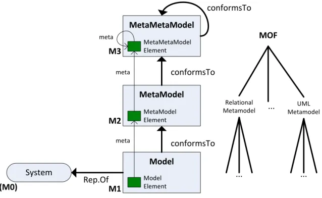
A model represents a system. To define a model it is necessary to define a metamodel, which describes all contained model elements, and the way they are arranged, related, and constrained. As models consist of elements, metamodels do too. The model elements are related to their conforming metamodel elements by meta-relations. So the element is typed by its metaelement. A model conforms to a metamodel if and only if each model element has its metaelement defined within the metamodel. Obvious a lot of different metamodels can exist (UML, PetriNets etc). This growing number makes it necessary to define the way, in which they are represented. One solution is a metametamodel, dedicated to the definition of metamodels. As models are based on metamodels, metamodels are based on a metametamodel. Since a metametamodel consists of elements too, a solution to represent metametamodels is needed again. To avoid a vicious circle, the OMG did introduce with MOF the four-level architecture. The MOF metametamodel is defined recursive, so it only exists of elements, which are typed by the MOF metametamodel itself. A typical solution based on the MOF four-level architecture exists of three layers of models11:

• M3: the metametamodel

• M2: the metamodels which conforms to the metametamodel • M1: the models which each conform each to a metamodel

(7)

2.1.4 Kernel MetaMetaModel (KM3) 7 MetaMetaModel System MetaModel Model conformsTo conformsTo conformsTo Rep.Of Model Element MetaModel Element MetaMetaModel Element meta meta meta M1 M2 M3 (M0) MOF Relational Metamodel UML Metamodel ... ... ...

Figure 2.2: the four-level architecture

MOF is often called a meta-modeling language. Those languages mostly are only distinct by small differences since they are generally based on the object oriented idea. (Meta)classes can contain attributes and are connected through references, which are also used for inheritance and typing. These meta-modeling languages generally only represent the semantic part. There are other languages to describe how to visualize the models and metamodels.

2.1.4 Kernel MetaMetaModel (KM3)

KM3 (Kernel MetaMetaModel) is another meta-modeling language, founded by INRIA. It’s based on the same concepts as MOF, for example the self-related property12. KM3 focuses on meta-modeling concepts and lacks some features of other meta-modeling languages, for example it doesn’t support Java code generation like the Ecore model. The use of KM3 is mainly justified by its simplicity and flexibility to write meta-models and to produce Domain-Specific Languages (DSLs). A lot of KM3 based metamodels are already preproduced and collected in the Atlantian Zoo13.

KM3 is a DSL to define metamodels. The domain definition metamodel is the KM3 model. The concrete syntax is a textual syntax defined through INRIA14. The semantic of KM3 is also defined and enables the specification of metamodels and models. KM3-models can easily be mapped to MOF and Ecore which makes KM3 usable with programs like Eclipse12.

(8)

8 2.2 Transformations

Example of an KM3-representation of a simple PetriNet metamodel

2.2 Transformations

A lot of different levels of abstraction and different kinds of models were mentioned in the last chapters. But there is something needed to glue all this together. Transformations make it possible to transform one or more models, the source, into other one or more other models, the target. The metamodel of source and target can be the same; in this case the transformation is called exogenous. If they differ the transformation is called endogenous15. A transformation contains all necessary information to map the source to the target in transformation-rules, which are based on a MTL (for example MOF/QVT or ATL). The MTL itself is based on a metametamodel and correlates with the metamodels of the source and the target which are based on the same metametamodel. A transformation engine later on uses the rules defined through the MTL to create the target model(s) out of the source model(s). A very important distinction can be made between model-to-model transformations and model-to-code transformation. Though it seems like a subset (because code can also be represented as a model) there is a momentous difference: while the former is a transformation on the same level of abstraction, the later changes this level.16 A good overview of transformations and some examples can be found in [17].

Transformations play a significant role in development automatisms. Especially as there are a lot of different metamodels used, MDE would be more inconvenient without it (I need a KM3-based model, you give me an Ecore-based model? No Problem, it is transferred with one click).

package SamplePetriNet {

class Net{

reference place[1−*] container: Place oppositeOf net;

reference transition[1−*] container: Transition oppositeOf

net; }

abstract class Arc {

attribute weight: String;

}

class Place {

reference net [*]: Net oppositeOf place;

reference out[0−*]: PTArc oppositeOf src;

reference in[0−**]: TPArc oppositeOf dst; }

class Transition {

reference net [*]: Net oppositeOf transition;

reference out[1−*]: TPArc oppositeOf src;

reference in[1−*]: PTArc oppositeOf dst; }

class PTArc ext ends Arc {

reference src [1]: Place oppositeOf out;

reference dst [1]: Transition oppositeOf in; }

class TPArc ext ends Arc {

reference src [1]: Transition oppositeOf out;

reference dst [1]: Place oppositeOf in; }

(9)

2.2.1 ATLAS Transformation Language (ATL) 9

2.2.1 ATLAS Transformation Language (ATL)

Conforming to INRIA ATL is a transformation-based model management framework, with metadata management and data mappings as the main applications18. It is general on a high grade of abstraction, making it possible to map to many different languages. It is consistent with many standards, especially the MDA MOF/QVT. ATL was released in 2004 as a part of AMMA (further information see [11]) under the Eclipse Public License which makes it Open Source. ATL comes with some Tools called ADT (similar to JDT), for example an Eclipse IDE, including and editor with syntax highlighting, an outline and simple wizards, and a debugger. Further ADT includes the ATL Engine19. A compiler produces byte code (.asm) out of an ATL-Project which can be executed on a virtual machine. The virtual machine can run on top of different platforms. Since ATL is used in this paper, it is focused on this transformation language.

An ATL Transformation is based on one or more ATL files (.atl):

• Module (the standard type, a normal module-to-module transformation) • Query (as the name implies a module-to-primitiveDataType transformation) • Library (can be imported by any type of ATL File including libraries itself)

An ATL Module consists of four parts: the header, the import, helpers and rules. They are described in the following paragraphs.

The header defines the name of the transformation and the input as well as the output models (also known as source and target models). The syntax for the input and output models is [variable name] : [metamodel name]. It is only possible to navigate through source models (which are consistently read only while target models are write-only).

The refine mode, enabled by the word “refines” (in contrast to “from”), allows he developer to save code, since unchanged elements are automatically copied from the source to the target. Corresponding to [22] section 3.1.2.2, the refine mode can only be used with a single source and a single target model which need to conform to the same metamodel.

The import section makes it possible to import various libraries. Later on, the imported helpers can be used in the module.

Helpers can be conceived as the equivalent to Java methods. Their name can be compared

to the name of the Java method, the return type defines the type of the return value (note: there is nothing like “void”). An ATL expression defines the computing part of the helper. The helper can also contain parameters, which are coded “[parameter name] : [parameter type]”. Since helpers can be invoked by other elements, the context describes the type of element, a helper can be called by, later accessible as “self”. If there is no context, the helper is invoked in context of the module itself. Helpers are deterministic and can be recursive.

helper [context context_type]? def : helper_name(parameters) :

return_type = expression;

module module_name;

create output_models [from|refines] input_models;

(10)

10 2.2.1 ATLAS Transformation Language (ATL)

The ATL expression syntax is very close to the OCL syntax. Further information can be found in [22] section 4.

If the parameter section is omitted, the helper is called “attribute”, something similar to a context specific constant. The main difference between attributes and helpers is that helpers are executed every time they are invoked. Attributes are only executed the first time they are invoked and later on only return the first calculated value.

Rules are the heart of a transformation. The typical rule is called “matched rule”. Such a rule

primarily matches a source pattern over source models and a target pattern that creates new elements in target models for every match. They comprise of four sections and although the “from” (source) and the “to” (target) sections are necessary the “using” and “do” sections are optional. The “from” section specifies the source element. The optional condition part makes it possible to distinguish between elements of the same type. Completing the manual, it is possible, to use elements of two different source-models in the “from” section. 20

The “using” section provides us with the opportunity to declare variables to use them later on in the rule.

The “to” section finally makes it possible, to create elements in the target models. It defines an arbitrary amount of target-elements and their bindings. The bindings can refer to the element(s) introduced in the “from” section. It is also possible to define a set of target model elements by using the word “distinct” and the corresponding syntax.

The “do” section makes it possible to define some additional imperative statements, which are run after the target model initialization has been finished. I don’t give their syntax in this paper.

module module_name;

create OUT : MM from IN1 : MM, IN2 : MM;

rule sample_two_input { from

a : MM!Element in IN1, b : MM!Element in IN2 (

[compare condition e.g.: a.name = b.name] )

... }

rule rule_name { from

in_var : in_type [(condition)]? [using { var 1 : var_type1 = init_exp1; ... var n : var_typen = init_expn; }]? to out_var 1 : out_type1 (bindings1), out_var

2 : distinct out_type2 foreach(e in coll.)(bindings2),

... out_var n : out_typen (bindingsn ) [do { statements }]? }

(11)

2.2.2 Higher Order Transformation (HOT) 11

If a matched rule is introduced by the word “lazy”, it has to be invoked by another rule. If it is introduced by the words “unique lazy” it can only be invoked once.21

In contrast to matched rules, “called rules” are only invoked by do-statements. There are two main syntax differences to normal rules: they have parameters and they don’t have a from-part. If called rules start with the word “entrypoint”, they are invoked at the beginning of the transformation22.Navigation is performed using OCL expressions.

As you can see, an ATL-transformation consists of declarative and imperative elements (do-statements and called rules) making it a hybrid technology, although it is highly recommended to use the declarative techniques whenever it is possible since they enhance the readability and matches better modeling. 23

Libraries contain several helpers and can be reused in modules, queries and even other libraries. They start with the expression library [library name] followed by an arbitrary amount of helpers. Queries are an easy way to extract primitive data from models, for example used to export strings. They are declared in the following way:

query [query_name] = [expression];

2.2.2 Higher Order Transformation (HOT)

Let’s reach another stage of abstraction: transformations are said to work on models. But we can think of transformations themselves as models, holding on the modeling paradigm “everything is a model”24. Transformations which have transformations as input and/or output are called HOT. They offer us a complete new prospect. For example it is possible to create metamodel independent transformations, which create a metamodel dependent transformation through a HOT based on a special metamodel as input. This technique is used in 4.3.

2.3 Model Weaving

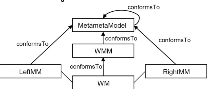
Figure 2.3: a weaving model is used to connect two models3

Model weaving is on another level of abstraction to transformations. The function of weaving models is to set precise correspondences between models or metamodels. A weaving model consists of typed links between model elements (it is possible to weave more

(12)

12 2.3.1 ATLAS Model Weaver (AMW)

than two models or metamodels11 but without loss of generality this paper relates to two metamodels). Differing from transformation, weaving models don’t imply a change from one model to another model creating a new one, but rather indicate a semantic relation between the corresponding models. In consequence, mapping information can be stored relatively simply, compared to a transformation language.

A typical usage of weaving models is shown in Figure 2.3. A weaving model maps two meta-models LeftMM and RightMM to each other, implying a fine grained relationship between those two metamodels. The weaving model conforms to a weaving metamodel which itself conforms to the same metametamodel as the connected metamodels. Since the weaving model is based on a metamodel, it is possible to use it as input for a transformation.

So the weaving model is not much more then a set of links between the two metamodels. In general, those links can’t be generated automatically because they are often based on human decisions, but in the most cases there are heuristics to approximate the result. Those heuristics check the signatures of elements, including name, kind and type. If there are several matches, structural similarity is used to construct the weaving model. Later, those automatically generated models can be fine-tuned by manual optimization. It’s even possible to match elements, which are normally not related, giving the developer extensive possibilities, for example pattern-driven evolution.25

2.3.1 ATLAS Model Weaver (AMW)

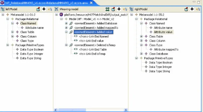
AMW is a component-based platform for model weaving, i.e. establishing and managing correspondences between models18. Simply said, it’s an IDE for Eclipse. After uploading the weaving metamodel, the GUI is established. Then the LeftMM and the RightMM can be chosen and the links can be established11.

(13)

2.4 Software Evolution 13

2.4 Software Evolution

Everybody who ever developed software knows that it is impossible to write correct and optimal software. Furthermore software which is correct in the eyes of the developer can fail in the eyes of the user. Today, most of the software is passed through many levels of development, not only the different phases of software engineering but also many different version identified by more or less small changes.

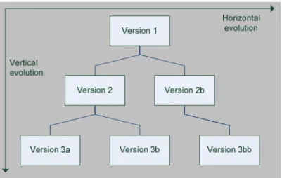
This software evolution induces high costs, making it worthwhile to have an intensive and accurate design phase before implementing the software. As mentioned in 2.1, this approach was often rejected because of short-termed higher costs in the designing phase, leading to an error driven development in the 90’s25. Nevertheless, even with an extensive design phase, it is not possible to create perfect software without implementing prototypes and even final versions, always including failures and a need to be maintained leading to a lot of different versions of a system. This incremental software evolution is called sequential evolution27. And can be thought of as the vertical dimension in a versioning tree. An example of this kind of versioning in everyday live is Wikipedia. If an article is updated by a user, the new version is saved, whilst the old version is kept in the system, making it possible to refer to a certain version of an article.

“Software versioning is the process of assigning either unique version names or unique version numbers to unique states of computer software. Within a given version number category (major, minor), these numbers are generally assigned in increasing order and correspond to new developments in the software. At a fine-grained level, revision control is often used for keeping track of incrementally different versions of electronic information, whether or not this information is actually computer software.”28

Today a lot of different developers are working on the same projects, bringing us to the next problem: the support for collaborative work or multi user access, resulting in a lot of different versions on the same vertical level, called parallel evolution27 (the horizontal dimension in a versioning tree). Necessarily special developing tools are needed to keep on track with the different versions, making it possible for several developers to work on the same parts of a project. Systems which solve this requirement are called Version Control System (VCS) or Source Code/Control Managementsystem (SCM)29 Those systems store the different versions on a centralized server, called the repository, making it possible to step back to any earlier state. Developers check out the actual version as their working copy. The local version can be held current by incremental updates from the repository. If the local working copy has reached a new level, the developer can commit his version to the repository (VCS do offer many further features, which are not mentioned in this paper).

(14)

14 3 Differences

Figure 2.5: a versioning tree

Some problems do appear, for example there is a need to handle the fact that several developers may want to work on the same data or files on the same time. One approach is the pessimistic revision control, meaning the file is locked while somebody is working on it, making it impossible to have two or more persons working on it30. It is used by versioning software like RVS or VSS. Optimistic revision control (e.g. used by CVS or SVN) uses the fact that two or more changes in a file might not influence each other. If a user tries to commit a file which was changed meanwhile, the system detects a version mismatch. In this case, there are three ways to handle the situation: either to throw away one of the two versions or try to merge them manually (supported by some tools) or automatically by heuristics (sometimes it is not possible to match them and a conflict arises). The third possibility is to start a new branch, meaning a new parallel version-tree, different to the so called trunk, which is the main developmental sector. For the sake of completeness it has to be mentioned that versioning and multi user access can be found in all kind of software and media (for example hypermedia documents31).

(15)

3 Differences 15

3 Differences

As explained before, Software can exist at different versions, which are stored in a VCS. As the word “different” implies, these versions are only separated by small differences. Differences are the way in which two or more things which you are comparing are not the

same32. Since it is contrary to equality, a change between two versions is needed. Storing the complete information to every version would be redundant; hence only one complete version and the differences between this and the other versions are stored. It’s one constraint of differences, that you can use the stored version V1 and the difference to another version V2 to calculate the complete version V2. And while this approach is transitive, it is possible to just store the difference to any computable version.

Differences can appear in varying fields. For example, most backup systems only store the information and data which changed. Most of today’s software does deliver their updates as so-called patches, nothing more then the differences to the installed version. Another example is the partial refresh of the GUI of most software systems. The use of differences has several advantages. First of all the space needed to store differences, is quite obvious smaller than the space needed to store the complete version. Secondly, it eases the testing and selection of software. The developer can easily select modifications to detect which ones corrupt the system. Finally, it helps to better understand the evolution the software undergoes, since the changes between two versions become clear, while the storage of two different versions must be compared in their entirety.

Sticking to software evolution, there are two kinds of approaches to using differences.

Forward differencing means, an initial version of the software is stored; later versions can be

computed by the appliance of differences. Since this approach seems rational, there’s some benefit to the second approach of backward differencing30. Contrary to the former, this approach uses a complete final version and differences to calculate the previous versions. The mentioned benefit lies in the fact, that the newest – therefore most accessed – version is always available. Furthermore, differences can be intensional, which means, they are based on a precise initial version, or extensional, which means, they can be applied to several revisions.

There are overall three ways of calculating differences30:

• Textual: the two versions are treated like text using tools like diff or vdelta to calculate the longest common substrings and calculating differences based on inserts and deletes of strings33. This approach does not support moving or changing operations.

• Syntactic: the two versions are compared in regard to there syntax, structure and their parse tree.

• Semantic: the two versions are compared on there semantic level, for example with

Semantic Diff34.

This thesis focuses on model driven engineering; hence it only surveys differences in models. Those models are mainly stored in XML (XMI) files. A structure-related calculation approach is needed. Also the problem of identifying objects has to be solved. In [35] a two step approach (including the detection of element mappings in step one) is illustrated.

A formal definition of model differenced versioning would be: M1 and M2 are models based on the same metamodel MM. The difference Δ from M1 to M2 can be calculated, formalized as Δ = (M2 – M1).

(16)

16 3.1 Difference Representation

Some information about traditional techniques and constraints in difference representation is presented in section 3.1, leading right into the model-independent approach this thesis is based on in chapter 3.2. In section 3.3 some basic application ideas are presented and in section 3.4 further operators to manage and work with differences are described, including Sequential Calculation, which is discussed precisely within this thesis.

3.1 Difference Representation

Once, the differences are calculated, it is necessary to store them. To gain the largest benefit, the used method should be independent of the calculation method on the one hand and conform to some requirements on the other hand. Referring to [3], those requirements are

• model-based, the outcome of a difference calculation must be represented as a model to conform to the spirit of “everything is a model” principle [12] and to enable a wide range of possibilities, such as subsequent analysis, conflict detection or manipulations;

• minimalistic, the difference model must contain only the necessary information to represent the modifications, without duplicating parts such as those model elements which are not involved in the change;

• self-contained, as a complement of the previous property, the difference must contain all the required information to autonomously represent the manipulations, without relying on portions of data contained in the compared models;

• transformative, each difference model must induce a transformation, such that when applied to the initial model it yields the final one. Moreover, the transformation must be applicable also to any other model which is possibly left unchanged in case the elements specified in the difference model are not contained in it. In other words, the transformation should give place to patch-like updates;

• invertible, each difference model must be invertible, such that whenever applied to the final model nullifies changes thus getting the initial model. Furthermore, all the information needed to obtain the inverse must be contained in the delta itself;

• compositional, the result of subsequent or parallel modifications is a difference model whose definition depends only on difference models being composed and is compatible with the induced transformations;

• meta-model independent, the representation techniques must be agnostic of the base meta-model, i.e. the meta-model the base models conform to. In other words, it must not be limited to specific meta-models, as for instance happens for certain calculation methods which are given for the UML meta-model;

• layout independent, the proposed mechanisms must be agnostic of the presentation issues, i.e. the concrete syntax defined for the difference meta-model. In other words, the solution must be not limited to specific visualization approaches, like edit scripts, coloured diagrams or delta trees.

The mentioned requirements imply some qualities, for example do minimalistic, self-contained and invertible imply the Dual Calculation and model-based and transformative properties satisfy the “everything is a model” paradigm. Meta-model and layout independent leads the way to use the method in DSM. The transformative property implies

(17)

3.2 Meta-Model Independent Approach 17

an automatic transformation TΔ induced by Δ so that M2 = TΔ(M1) is imperative (with M1 and M2 are models conforming to the same metamodel).

Property edit scripts colouring

model-based NO YES

minimalistic NO NO

self-contained NO NO

transformative NO NO

invertible YES YES

compositional YES NO

meta-model independent NO YES

layout independent NO NO

Table 3.1

There are two major techniques to visualize differences, directed and symmetric deltas28. Directed deltas can be compared to a step-by-step recipe to prepare the new model. Normally it’s a list of add, delete and edit commandos, which transform a given model into a new one. Since it’s linear and text-based, it is quite easy to optimize it or to compose it. On the other hand, the directed approach lacks in clarity and is pretty hard to read for a developer (which lowers the benefits of using differences). There are also some further disadvantages as use of direct identification, which makes this approach impractical for interoperable differences.

In contrast, symmetric deltas use a highly visual technique, representing the initial and the final model while coloring the changes. For example, all elements, which appear in the initial model but not in the final model, are colored red, showing that they are deleted. All elements, which did not exist in the initial model, but appear in the final model, are colored green, meaning they are added etc. Although this approach is highly readable, it is in no way minimalistic or easy to compose. So there’s a need to develop a new approach, which fulfills all the announced properties.

3.2 Meta-Model Independent Approach

It is necessary to find a general approach to model differences, which fulfill all the mentioned properties. Talking about “modeling” differences is possible, since we are only working with models, according to the MDE paradigm “everything is a model”. Staying on this, we can consider the differences have to be represented as a model, too. Models always conform to a metamodel, and so too must the differences.

A unified method to represent metamodels was already announced in 2.1.3; hence to have a unified and metamodel-independent approach to represent and store difference models, we need to have a method to construct difference metamodels out of arbitrary metamodels. This method is presented in this section.

3.2.1 Difference Metametamodel (MMD)

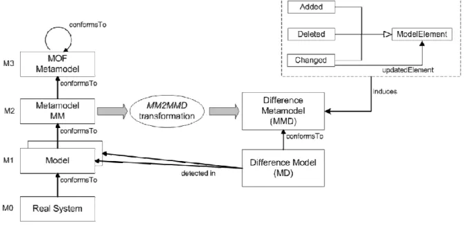
Difference models are positioned on the level M1 of the four-level architecture. So, the difference metamodel has to be positioned on the level M2 (see Figure 3.1). To represent differences, every modeling element (conforms to the “class-type” of the KM3 model) of the original metamodel MM needs options to add or delete it. Furthermore, to not always delete and re-add an element, if one or more characteristics did change, a change-option is

(18)

18 3.2.2 Constructing Constraints/Rules

needed as well. The easiest way to fulfill these needs is to construct a difference metamodel which is the original metamodel with every contained element MC complemented with the following subclasses

• AddedMC, if a new element is added in the final model, which is not present in the initial model, it is done by using the corresponding AddedMC class in the difference model.

• DeletedMC, if an element is deleted, meaning it existed in the initial model but disappears in the final model, it is done by using the corresponding DeletedMC class in the difference model.

• ChangedMC, an element in the final model can differ from the corresponding element in the initial model. In this case, the old element is represented in the difference model in form of a ChangedMC element, which contains all attributes and references, which shall be deleted, and which relates via the reference

updateElement to an element of the MC class, which contains the new added

attributes and references.

Figure 3.1: Difference metamodel generation3

An ATL transformation to construct a difference metamodel out of any metamodel based on KM3 is given in [36]. The ATL transformation MM2MMD (Metamodel2MetamodelDiff.atl) builds a difference metamodel MMD by copying all elements of the original metamodel MM. Furthermore, three classes AddedMC, DeletedMC and ChangedMC are added for every non abstract class in MM. These new classes are subclasses of the original class MC on the one hand and of their respective abstract class Added, Deleted or Changed, which are also added to MMD on the other hand. To handle ordered references, it is necessary to add the position index to the ordered classes (compare figure 4.9 in [3]).

3.2.2 Constructing Constraints/Rules

• model-based, meta-model independent and layout independent, easy to see, that the difference model is a model itself and that this approach is metamodel independent since it can be applied to all metamodels. Layout independence is given through the

(19)

3.2.3 Example 19

fact that difference models can be easily calculated to any arbitrary visualisation like colouring or editing scripts.

• minimalistic, self-contained, invertible, difference models are by definition minimalistic and self-contained. For example, if a container is deleted, all contained elements need to be deleted, too, in the delta, since otherwise the self-contained and so the invertible properties would not be fulfilled.

• transformative, for every difference meta-model, a transformation can be automatically derived, so that the final model can be calculated by the use of the initial model and the difference model as input.

• compositional, is given, too. For example the Sequential Calculation is discussed extensively in this document.

3.2.3 Example

This is a simple example based on the simpleUML example, which can be found in [3] in chapter 4, Figure 4.6 and 4.8 (including larger examples).

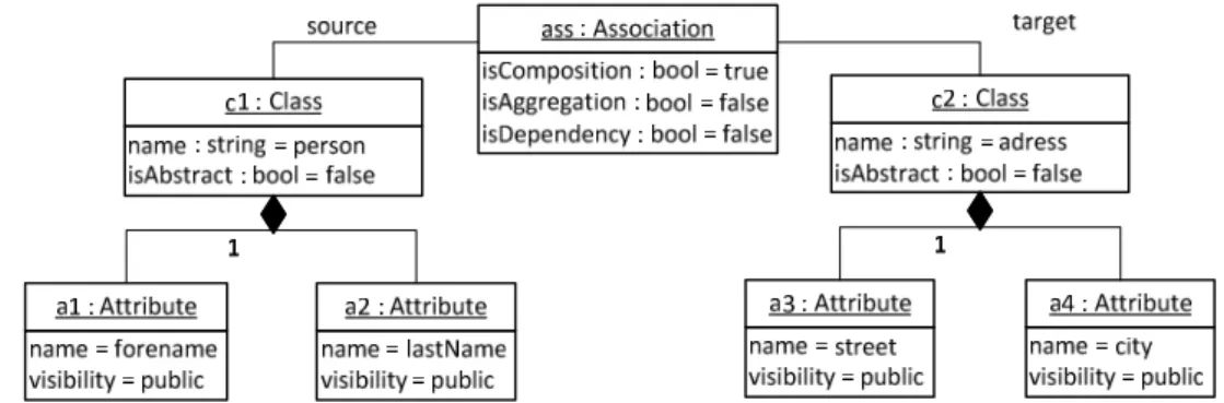
Figure 3.2: Initial model m1 of a person with a address

In Figure 3.2 an initial model m1, based on the simpleUML metamodel is presented. It consists of a Class person, which has forename and lastName Attributes. It’s associated with a Class address, which consists of the Attributes street and city. This initial model shall be changed to a new model m2. For some reason lastName is changed to surname and we don’t want to store the address anymore. Instead, we want to store contact information, for example the phone number. This model can be seen in Figure 3.3

Figure 3.3: final model m2 of a person with contact information

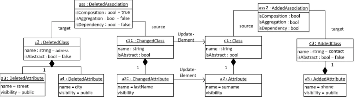
Obviously, there are some changes, which need to be stored in a difference model. First of all, the Class c2 and the belonging Association ass are deleted. A new Class c2 and its belonging Association ass2 and its Attribute a5 are added. Finally, the Attribute a2 is changed. So let’s have a look at the difference model Δ in Figure 3.4:

(20)

20 3.3 Difference Application

• Not only the Class c2 is deleted but also its contained Attributes a3 and a4 need to be deleted, due to the self-contained property described in 3.1. This is necessary to enable the Dual Calculation described in 3.4.1.

• The class c1 is also changed, although none of its properties are changed. This is necessary because one of its contained elements is changed and because a referenced Association is changed.

Figure 3.4: difference model Δ

3.3 Difference Application

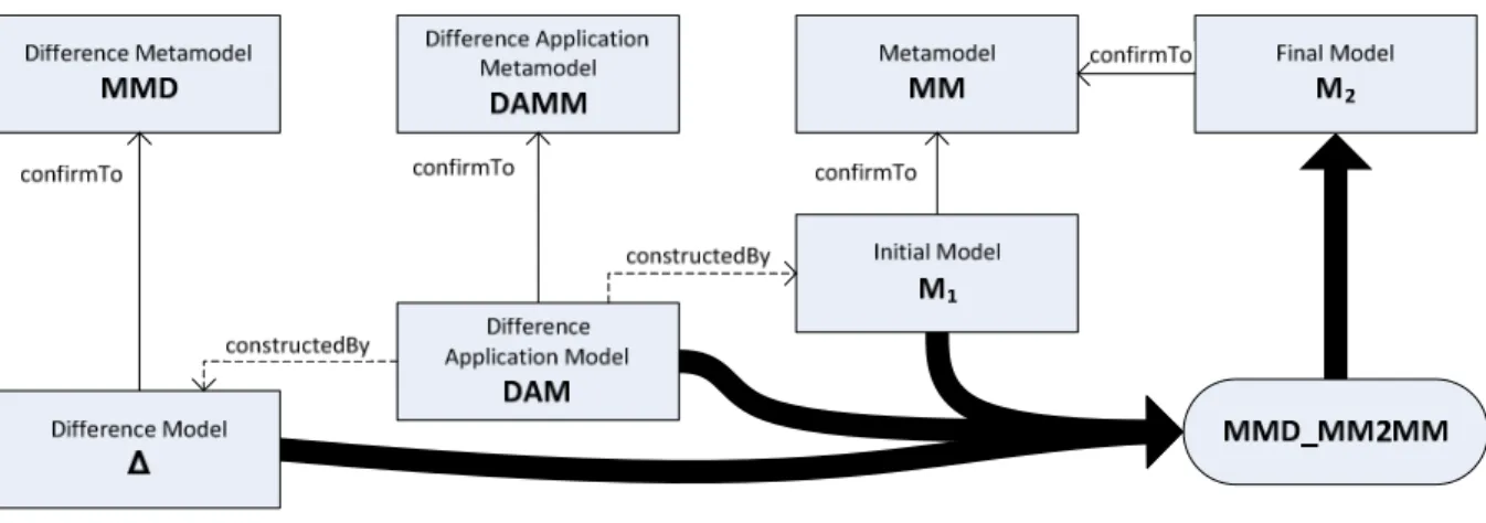
After discussing the concept and the construction of differences, it’s necessary to point out the benefit of them: how to use them, to transform one model into another one. Looking at Figure 3.5, the process of difference application becomes clear: a model M1 and a difference model Δ are matched in the MMD_MM2MM transformation to obtain a new model M2. Δ is calculated by computing the differences between two original models, Δ = M2’ – M1’. Model weaving leaves the door wide open to many possibilities, since M1 and M1’ don’t have to be the same models, they just need to conform to the same metamodel and can later be connected through a weaving model DAM:

• Reconstructive application is the standard way to weave them together. In this case M1 = M1’, and Δ matches completely against M1 without any further weaving. Hence M2 = M2’. This would be the normal way in software versioning. One model is stored and the other models can be obtained by the use of the differences, calculated out of exactly the same models.

• Idempotent application is the second and easy case: M1 ∩ M1’ = Ø and the weaving model is empty. Thus the difference application will only add elements, described in MD. If there are no AddedMCs in MD, M1 = M2.

• Transformative application: if M1 ∩ M1’ ≠ Ø, it is possible to realize a patch like application. The changes would only affect elements in the set M1 ∩ M1’ and M2 ∩ M2’ ≠ Ø. A special case of this would be M1’ ⊆ M1 with the result M2’ ⊆ M2. Weaving techniques make it possible that there could also be matches even if M1 ∩ M1’ = Ø, if elements from M1 and M1’ are connected in the weaving model. Transformative application can lead to several conflicts, for example, if Δ deletes an element, which exists in M1’ but not in M1, so model weaving has to be done very carefully.

(21)

3.4 Operators 21

Figure 3.5: an overview of the difference application process

After describing the whole transformation process, let’s specify the MMD_MM2MM. This transformation is calculated by the HOT MMD2ATL, which gets the used difference metamodel MMD as input and outputs the corresponding MMD_MM2MM. A specific MMD_MM2MM transformation gets three inputs: an initial model, a difference model and a weaving model to connect them. For every class MC in the original metamodel, there are three rules in the MMD_MM2MM file (in this case, Δ means all differences, including those who are matched by model weaving):

• AddedMC2MC: creates for each AddedMC element in Δ a new instance of MC in M2, according to the specifications of AddedMC.

• ChangedMC2MC: creates for each ChangedMC element in Δ a new instance of MC in M2, according to the original specifications of MC in M1 considering the changes which are done in ChangedMC and the associated updateElement.

• UnchangedMC2MC: copies all elements, which have to be the same in M1 and M2, hence all elements MC in M1 which don’t have a related ChangedMC or DeletedMC in Δ.

It is easy to see, that all elements are able to be well dealt with: added elements because of the AddedMC2MC rule, changed elements because of the ChangedMC2MC. Deleted elements are not copied to the M2 because of the restrictions in UnchangedMC2MC. Further information can be obtained in [3], section 5.2.

3.4 Operators

As mentioned before the evolution of software can consist of one complete version and differences to calculate the other versions. There are some techniques to ease the handling of those steps. First of all, we need a formalized definition of a delta:

Δ = (M2-M1)

This means, the difference between an initial model M1 and a final model M2 both conforming to the same metamodel MM, is stored in the delta Δ, conforming to a difference-metamodel derived from MM. The final model M2 can be calculated by using M1, Δ and a transformation T:

M2 = TΔ(M1)

The Dual Calculation makes it possible to automatically generate an inverse of a difference, making it possible to switch from forward to backward differencing and the other way

(22)

22 Sequential Calculation

around or to simply undo last changes. Sequential Calculation and Parallel Calculation are two techniques, to merge several differences. Whilst the former uses linear grouping methods, the later merges two concurrent and competing differences on a horizontal level.

3.4.1 Dual Calculation

As mentioned before, we assume a transformation TΔ between M1 and M2 with Δ representing the difference between M1 and M2. While M1 and M2 are models, conforming to the same metamodel MM, TΔ conforms to an automatically generated difference metamodel MMD. Since we defined in 3.1, that a difference needs to be invertible, we induce the dual or inverse of the delta Δ as Δ-1. It is necessary to distinguish between the inverse of a difference representation and a inverse of a difference application. Whilst the former is our introduced inverse or dual representation of our difference, the latter is the undo-function, which can be formalized as T-1Δ with M1 = T-1Δ(M2). Since we define Δ-1 as the inverse of Δ, we can assume, that M1 = TΔ-¹ (TΔ (M1)) or in other words, the successive use of the difference and its dual nullifies the changes. So we can emulate the undo-function T-1 by using the dual representation. Hence TΔ-¹ (x) = T-1Δ(x). In this thesis, the undo operation is completely displaced by the transformation operation with the calculated dual of the last delta. This technique brings some benefit:

• The undo operation does not stick any more to a particular tool since every tool can implement the calculation of the dual from the difference.

• The undo operation does not need to store any more information since all needed information is stored in the delta itself.

• The dual difference matches the representation properties mentioned in 3.1 by construction; therefore it can be used in any way.

By looking closer to the dual calculation, it becomes obvious, why we want to record all and only the changes between the two compared versions. For example, it would be minimalistic to only store the deletion of a container and not the contained elements since the deletion of those could be automatically done. But it wouldn’t keep the self-contain or invertible conditions since the deletion of the contained elements is not contained in the delta, there wouldn’t be an adding of those elements in the dual delta. So those element would be missed in M1 if we execute M1 = TΔ-1 (TΔ (M1)). It’s obvious, that every single element, which gets deleted or added, needs to be stored in the delta.

Relating to section 3.2, the dual calculation can be easily calculated: every AddedMC becomes a DeletedMC. Contrariwise, every DeletedMC becomes an AddedMC. The ChangedMC and the corresponding updateElement MC change position, or in other words: the ChangedMC is transformed into MC, the corresponding MC is transformed into ChangedMC and the updateElement relationship between them is reversed.

3.4.2 Sequential Calculation

There are possible circumstances where it is necessary and convenient, to group several deltas, which would be executed sequentially, into one simplified delta. The concept, calculation and furthermore optimization of this sequential delta will be extensively elaborated in chapter 4. At this point, it’s just necessary to introduce a sequential operator “;” which merges given Δ1 and Δ2 in the following way:

Δmerged = Δ1 ; Δ2.

Without loss of generality we can assume in the further discussion m1, m2,m3 are models,

(23)

difference-3.4.3 Parallel Calculation 23

metamodel MMD, derived from MM. In this text, Δmerged is also called the new delta; m1 is called the initial model; m2 is called the middle model and m3 is called the final model. They are connected in following way:

• Δ1 = (m2 – m1): the difference from m1 to m2 • Δ2 = (m3 – m2) : the difference from m2 to m3

• Δmerged: the optimal difference derived by merging Δ1 and Δ2

As the merged delta shall be optimal, Δmerged = (m3 – m1) must be valid. Furthermore it is essential, that TΔ1; Δ2 = TΔ1 * TΔ2 with “*” being the concatenation of two transformations. Referring to

Figure 3.6 it is easy to see, since TΔ2(TΔ1(m1)) = m3 = TΔmerged(m1).

Figure 3.6: sequential composition

3.4.3 Parallel Calculation

Often it is not possible to tell the order of two or more deltas which need to be applied. Hence, a sequential approach is not practical. For example, it’s quite common that several developers work on the same data or rather files, as mentioned in 2.4. Since locking of the file is impractical, it’s possible that two or more developers create a new version which leads to a new delta in each case. If those deltas are merged back to the repository, parallel calculation is used to get the actual result. Another example is the case when a branch is merged back into the trunk. In this case, sequential and parallel steps can even be combined, since first, the sequential steps in the branch are merged and later on, the final branch delta and the trunk delta can be merged in parallel. Similar to the sequential operator, a parallel operator does exist: Δmerged = Δ1 || Δ2.

If the changes don’t interfere to each other, they are just merged (they could be treated as two sequential deltas where the order does not matter. Formalized this can be written as Δ1 || Δ2 = TΔ1; Δ2 + TΔ2; Δ1 with “+” being a non deterministic choice between the given merged deltas. If changes interfere, this solution is not practicable because syntactic and semantic conflicts may arise37.

(24)

24 4 Sequential Calculation

4 Sequential Calculation

Software evolution is one of the main targets for differences. As discussed in 3, there are several advantages in storing only one complete version plus the differences to calculate the other versions, for example the reduction of needed storage space. If the use of forward differencing is assumed (without loss of generality, see 3.4.1), it is necessary to consecutively apply every single difference in the version history to get the final version. To change from one version to another one - skipping some intermediate steps - it would be more favorable, to have an easy way to calculate one single difference, including all the needed information. Another example is the use of differences technology as software patches as mentioned in 3.3. If the actual deployed version is known, it is most easy to roll out a single difference, which represents the sequential calculation of all differences between the actual deployed and the actual developed version. The sequential calculation is also specified in the difference property compositional in 3.1.

For the sake of simplicity, we are assuming two deltas which are merged. It is easy to see that we can extend this approach to an arbitrary amount of deltas through concatenation. To prove this, we need the “;” sequential operator to be associative, hence (Δ1;Δ2);Δ3 = Δ1;(Δ2;Δ3). It is easy to see, that this must be true because of minimalistic and self-contained properties, so a proof is set aside. Considering the associativity, we can prove the statement by mathematical induction:

• Statement: we can connect an arbitrary amount of deltas Δ1 … Δn to a new delta ΔnMerged = (Δ1 ; … ; Δn) by the sequential operator, which connects two deltas.

• Basis: n=2 (n=0 and n=1 are trivial): Δ2Merged = (Δ1 ; Δ2) is given by the definition of “;” • Inductive step (n->n+1):

Δn+1Merged

= (Δ1; … ; Δn ; Δn+1) = (Δ1; … ; Δn) ; Δn+1 = ΔnMerged ; Δn+1

• Conclusion: an arbitrary amount of deltas can be merged by merging two deltas to a new one and merge this new delta with the next delta and so on. q.e.d.

This approach is similar to the well-known divide-and-conquer algorithm38. The overall problem of merging several differences is divided into several small problems of merging two differences. This job can easily be “conquered” (solved) as later on shown.

4.1 Concept

For the sequential calculation of two deltas into a new delta there are only the source deltas (Δ1, Δ2) and the conforming difference-metamodel MMD required. The calculation can be computed completely independent from any models or metamodels where Δ1, Δ2 and MMD were created by.

The Differences themselves can contain the original classes (MC) or their derived classes (addedMC, deletedMC and changedMC). Let’s call contained(Δx) the set of all original

classes, which are either self contained in a delta Δx or represented by a derived class contained in Δx. If an intersection of contained(Δ1) and contained(Δ2) equals the empty set, the deltas are sequential independent, formalized as contained(Δ1)

∩

contained(Δ2) = Ø. If

(25)

4.1.1 Constraints 25

this is the case they can just be merged; hence all contained classes of Δ1 and Δ2 are copied to the new delta Δmerged.

If contained(Δ1) ∩ contained(Δ2) ≠ Ø, some optimization can and must be applied, regarding to the minimalistic property introduced in 3.1. Effectively, all information to calculate the intermediate steps needs to be deleted or rather not copied.

Class-based objects can belong to one of five forms in every delta: the MC itself, AddedMC, DeletedMC, ChangedMC or they do not appear.

If an object (in whatever form) does not appear in either Δ1 or Δ2, the object itself is sequentially independent and can be copied into Δmerged in the form in which it exists in the other delta.

Deltas are a way to describe adding, deleting and changes. If an element appears in a delta in its original form MC, there are several reasons:

• It’s referenced by either a changed Element or an added element with one way association (by two way association, it would be of the type ChangedMC). So in fact, the element itself does not appear in the difference but only the reference to it. Hence, it can be treated as though it won’t exist in the delta.

• It is an updateElement of a ChangedMC. In this case, it’s included in the treatment of the ChangedMC element.

So finally there are the three derived forms (AddedMC, DeletedMC, ChangedMC) left, which leads us to 9 (= 3²) combinations, which are considered in section 4.2.

4.1.1 Constraints

Cicchetti mentions in section 4.2 of [3] that a calculated composite, like the sequential composite, needs to be valid data, thus conform to the same meta-model the composed documents conform to, which means Δ1, Δ2 and Δmerged do need to confirm to the same difference-metamodel. Also all properties introduced in 3.1 must be observed:

• minimalistic: there are no elements added, which are not already elements of Δ1 and Δ2. Dispensable information, which can arise through the composition of two elements, is prevented by an optimized merging process;

• self-contained, since all elements are copied and only the redundancies are reduced, all needed information is stored;

• transformative: the used transformation can be the same as used for Δ1 or Δ2 since the deltas are based on the same difference-metamodel. Based on the fact, that Δ1 and Δ2 would leave models without elements specified in the difference models unchanged and the fact that no elements (in whatever form) are added, we can consider the transformative property to be upheld.

• Invertible: the optimization process makes sure, the Δmerged is self-contained and minimalistic, making it possible to calculate the dual representation the same way it is calculated for Δ1 or Δ2.

• Compositional: A very important property since this is the basis for merging more then two deltas: Δmerged itself is compositional and can be merged with every proper delta;

• model-based, meta-model independent, layout independent, Δmerged does only consist of elements which are found in Δ1 or Δ2 and uses the same representation technique, hence, these properties are fulfilled.

(26)

26 4.2 Cases

Considering the dual calculation ( TΔ1-¹(m2) = m1 and TΔ2-¹(m3) = m2) also some constraints over dual calculation can be done (remember Δmerged = (Δ1 ; Δ2) hence Δmerged-1 = (Δ1 ; Δ2)-1)

• TΔmerged-¹(m3) = m1: the inverse of the sequential concatenation needs to transform the final model back into the initial one since the sequential concatenation itself transforms the initial model into the final one.

• (Δ1 ; Δ2)-1 = (Δ2-1 ;Δ1-1): thinking of the undo operation, it becomes obvious that to get back from m3 to m1 by single steps, first the changes done by Δ2 have to be reversed to get m2 and afterwards the inverse of Δ1 needs to be applied to reach the initial model m1. This means, that the inverse Δmerged-1 can be calculated by inversed sequential concatenation of the dual representation of Δ1 and Δ2, hence (Δ1 ; Δ2)-1 = Δmerged-1 = (Δ2-1 ; Δ2-1).

4.2 Cases

As mentioned in 4.1, there are nine cases obtained by combining all remaining classes with each other. They are composed in Table 4.1. The nine cases can be divided into two families: the existing and the non existing family. Elements of the former family can appear. It is necessary to research in which way the according element in Δmerged can be calculated. All four elements of the latter can’t exist, represented in Table 4.1 by “–“. Nevertheless it is necessary to prove, that they can’t exist.

Δ1/Δ2 AddedMC ChangedMC DeletedMC

AddedMC – AddedMC null

ChangedMC – null/ChangedMC DeletedMC

DeletedMC null/ChangedMC – –

Table 4.1: possible cases of sequential composition

4.2.1 Existing

As a side remark, ordered references are presented through an attribute positionIndex (compare chapter 4.4 of [3]). Hence they are covered by considering attributes and references in the following paragraphs.

• AddedMC + ChangedMC: an element is added in Δ1 and later on changed in Δ2. Since this element is added first, it did not exist in the initial model. Hence the new element in Δmerged needs to be of the type AddedMC, too. On the other hand, the changes in the ChangedMC must be paid attention: all attributes and references which are changed in the ChangedMC must be changed in the new AddedMC compared to the original AddedMC. All other parts of the original AddedMC can just be copied to the new one.

• ChangedMC + DeletedMC: inversely to AddedMC + ChangedMC element is deleted in Δ2, so it does not appear in the final model. Hence the new element in Δmerges needs to be of the type DeletedMC, too. Since the element, which is deleted in Δ2 differs from the element which needs to be deleted in Δmerged, all changes in attributes and references which appear in ChangedMC must be treated in the new DeletedMC. • AddedMC + DeletedMC: the element is added in Δ1, so it did not exist in the initial

model. It is deleted in Δ2, so it does also not exist in the final model. Hence, it mustn’t appear in the Δmerged.

• DeletedMC + AddedMC: if the element, which is added in Δ2, has exactly the same attributes and references then the one which is deleted in Δ1, there is no change in the models and the element mustn’t appear in the Δmerged. If there is a change,

(27)

4.2.2 Non Existing 27

DeletedMC is copied to Δmerged as new ChangedMC and AddedMC is copied to Δmerged as the corresponding updateElement MC. Attributes or references which do not differ mustn’t be copied.

• ChangedMC + ChangedMC: if ChangedMC in Δ2 nullifies the changes made by the ChangedMC in Δ1, the element mustn’t appear in the new Δmerged. In other words, if the calculated dual or reverse of the one ChangedMC equals the other ChangedMC, both can be ignored. If there are differences, a new ChangedMC need to be constructed in Δmerged: Let’s assume chgx are the set of attributes and references

which appear in the ChangedMC in Δx and updx are the attributes and references that

appear in the updatedElement MC in Δx. Consider that chgx-updy means all elements which appear in chgx but not in updy. Two construction rules can be defined (see Figure 4.1)

o chgmerged = (chg1-upd2) + (chg2-upd1). o updmerged = (upd1-chg2) + (upd2-chg1).

Figure 4.1: concatenation of two changed classes

4.2.2 Non Existing

• AddedMC+AddedMC: it is impossible to add an element which already exists in a model. Since the element is added in Δ1, it exists in m2. Hence it can’t be added in Δ2 according to the definition, Δ2 is the difference from m2 to m3.

• ChangedMC+AddedMC: After the change of an element, the element does still exist (unlike when it is deleted). So the element still exists in m2 and hence can’t be added in Δ2.

• DeletedMC+ChangedMC: the change operation in Δ2 needs an existing element in m2. Since the element was deleted in Δ1 it does not exist anymore in m2.

• DeletedMC+DeletedMC: to delete an element in Δ2, the element must exist in m2. Since it is deleted in Δ1, it doesn’t exist in m2.

4.2.3 Examples

This chapter presents some examples to the sequential composition cases. For Figure 4.2 and Figure 4.3 an empty initial model and for Figure 4.4 and Figure 4.5 an initial model with only a class c1 (name=”class1”, isAbstract=”false”) can be assumed.

Figure 4.2 shows the AddedMC + ChangedMC case. In Δ1 a class c1 is added with the attributes name = class1 and isAbstract = false. This attribute is changed in Δ2 to class1b. In Δmerged those two differences are merged. Since there was no class c1 in the initial model and there is one in the final model, a class needs to be added in Δmerged. This class has the

isAbstract value of the AddedClass in Δ1, but since the name was changed in Δ2 it features the new value class1b.

Figure 4.3 shows the case, where a class is added in Δ1 and exactly the same class is deleted afterwards in Δ2, hence this class does not need to appear in Δmerged (it can’t be deleted or