SKI Report
SSI Report
2005:39
2005:08
Research
Large-Scale Groundwater Flow with Free
Water Surface Based on Data from SKB's
Site Investigation in the Forsmark Area
Anders Wörman
Björn Sjögren
Lars Marklund
December 2004
SKI-perspective
Background
SKI and SSI the two authorities that review and monitor SKB’s work related to the final repository for high-level nuclear waste. An important part of the final repository
concept is to be able to describe the large-scale transport of radionuclides that may occur as a result of a possible future leakage from the repository. SKI has throughout the years financed a number of projects within this area (e.g., SKI-report 2004:14, i.e. Wörman, 2005). Other important issues are to identify discharge areas in the landscape as well as pathways for radionuclide transport to various ecosystems and the resulting radiological doses to humans. To address these issues SKI, together with SSI, took the initiative to this research project, with the general objective to develop a large-scale transport model that can describe catchment scale radionuclide transport. The model will account for both surface hydrological processes and processes occurring in the geosphere-biosphere interface, and thus the effect of these processes on the deep
groundwater flow pattern. SSI will then use the results from this transport model in their ecological models.
Objective
The overall purpose of the project is to link small-scale retention phenomena and groundwater circulation with large-scale pathways for radionuclides and turnover in ecosystems as well as doses to humans.
Results
This report describes the first part of the project that comprises the development of a database and the part of the model used to simulate groundwater flow.
Relevance for SKI
SKI will use the results from this project in its continuous review and monitoring of SKB’s work within this field.
Future work
The continuation of the work reported here is described in the project SKI 2005/190/200509005.
Project information
SKI project manager: Eva Simic. SSI project manager: Shulan Xu.
SKI Project Reference: SKI 14.9-031125, project number: 200309008 SSI Project Reference: 60/3461/03, project number: SSI P 1422.04
Research
Large-Scale Groundwater Flow with Free
Water Surface Based on Data from SKB's
Site Investigation in the Forsmark Area
Anders Wörman
Björn Sjögren
Lars Marklund
SLU
Avd. för biometri och teknik
Box 7070
750 07 Uppsala
Sweden
December 2004
SKI Report
SSI Report
2005:39
2005:08
This report concerns a study which has been conducted for the Swedish Nuclear Power Inspectorate (SKI) and the Swedish Radiation Protection Authority (SSI). The conclusions and viewpoints presented in the report are
Sammanfattning
Denna rapport beskriver en databas som täcker hela Sveriges yta med avseende på olika geografiska parametrar av betydelse för simulering av grundvattenströmning på en regional skala och i hela kontinentalplattan. Databasen innehåller topografi,
vattendragen definierade i nätverk, markanvändning och vattenkemi i grundvattnet på begränsade områden.
Dessutom innehåller rapporten en beskrivning av ett beräkningsprogram som löser kontinuumekvationerna för laminär, stationär och isotrop grundvattenströmning. Formuleringen tar hänsyn till en fri grundvattenyta utom där denna strömmar ut i vattendrag samt sjöbottnar.
Modellens teroretiska bakgrund och koderna finns beskrivna. Beräkningsmiljön är Matlab. Rapporten ger även en bruksanvisning (manual) för koderna och ger ett beräkningsexempel från Forsmarksområdet, Uppland.
Summary
This report describes a data-base that covers entire Sweden with regard to various geographical parameters with implications to simulation of groundwater circulation on a regional and continental scale. The data-base include topography, stream network properties, and-use and water chemistry for limited areas.
Furthermore, the report describes a computational (finite difference) code that solves the continuum equation for laminar, stationary and isotropic groundwater flow. The
formulation accounts for a free groundwater surface except where the groundwater recharge into the stream network and lake bottoms.
The theoretical background of the model is provided and the codes are described. The report also contain a simple user manual in a Matlab environment and provides and example calculation for the Forsmark area, Uppland, Sweden.
Content
1 Introduction... 1
1.1 Background and project purpose ... 1
1.2 Objectives with database... 1
1.3 Objectives and limitations of flow model... 3
2 Database... 4
2.1 Area and coordinate system ... 4
2.2 Elevation data... 5
2.3 Land use ... 6
2.4 Underlying data used for streams and lakes ... 7
2.5 Conversion of data from Shape format to Matlab ... 9
2.6 Treatment of disjunctive stream network and file type ... 9
2.7 Strahler order ... 12
2.8 Summary of were to find data in the database ... 12
3 Description of groundwater flow model ... 14
3.1 Physical background ... 14
3.2 Numerical methods ... 15
3.3 Verification of numerical accuracy using closed-form solutions ... 19
4 Simple user guide for computer codes ... 22
4.1 Indata... 23
4.2 Executing the programmes ... 24
4.3 Forsmark calculation example ... 24
5 Description of codes for groundwater flow ... 27
5.1 Definition of boundary geometry and grid net ... 27
5.2 Definition of boundary conditions ... 30
5.3 Assembling of equation system and solution algorithm ... 34
5.4 Particle tracking ... 36
6 Results and concluding remarks... 37
7 References ... 38
Appendix 1: Files required for Groundwater Flow Simulation... 39
Matlab .m-files ... 39
1 Introduction
1.1 Background and project purpose
An essential issue for the site selection of the final repository of spent nuclear fuel and associated safety analyses is the large-scale migration behaviour of radionuclides from a leaking repository. Coupled and equally important issues include the water discharge areas in the landscape and pathway distributions for radionuclides to ecosystems as well as radiological doses to individual humans.
As a part of the R&D activities of the Nuclear Power Inspectorate (SKI) a research project was initiated with the overall purpose to develop a transport model on the geosphere-watershed scale. The model should be able to address the impact of surface hydrology and, particularly, the geosphere biosphere characteristics (surface
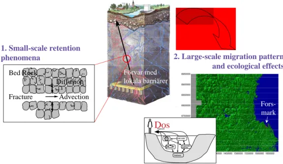
topography, thickness of quaternary deposits, etc.) on the circulation of deep groundwater. The project is initiated in collaboration with the Swedish Radiation Protection Agency (SSI) and one of the purposes behind this collaboration is that the results of the current transport model can be made available to ecological models developed by SSI. In this way, the overall purpose of the project is to link small-scale retention phenomena and groundwater circulation with large-scale pathways for radionuclides and turnover in ecosystems as well as doses to humans (Fig. 1). This report describes the first part of the project that comprises the development of a data-base and the part of the model used to simulate groundwater flow. The report includes a description of physical background to the problem as well as a brief description of the computational codes in a Matlab-environment.
The reactive transport model is a later progress of this project and is not treated here. Partly, the reactive transport model has been developed in previous SKI research projects (Wörman et al., 2004). The data-base is based on the SKB site investigation currently in progress in the Forsmark area, but includes also several types of
geographical information for a large part of Sweden. The reason for this are the facts that 1) the motion of deep groundwater is governed both by local conditions and large-scale (continental) motions of water and 2) generally accepted watershed boundaries do not apply to groundwater with the same significance as for surface water.
1.2 Objectives with database
The groundwater motion in bedrock is governed by the continental characteristics of the sub-surface environment and the infiltration distribution. In the Swedish part of the Fennoscandian shield, the overall direction of the flow is from the Scandinavian mountain range towards the Baltic Sea that acts as recipient for all groundwater (Provost and Voss, 2001). The flow pattern is complicated by local heterogeneities in the bedrock, like fracture zones, and variation in surface hydrology, such as connections to streams and infiltration distribution.
An essential empirical basis for testing of the proposed model development and more specific studies is the data base developed by SKB from their site investigations at Forsmark and Oskarshamn. Another important source of information comes from the
National Land Survey of Sweden. Such site-specific field data will enable plausible analysis of the effects of surface hydrology and, particularly, the geosphere-biosphere characteristics on the circulation of deep groundwater. These effect analyses, not presented in this report, will be generic in the sense that the model environment is just based on a limited amount of data not necessarily the best geomorphological and geochemical representation of the specific sites.
This report describes the data-base for the Forsmark area and is focused on the following types of geographical data:
• Ground surface elevation (topography of the landscape) • Land-use
• Streams, particularly stream network characteristics • Position of lakes and wetlands
Other types of data that potentially will be important in this project, but not treated in this report, include
• Infiltration data as function with position in the landscape or alternatively related surface hydrological parameters
• Geological interpretative model (hydraulic conductivity or similar), such as a discrete fracture model or any other geological model including quaternary deposits
Figure 1. Schematic of the overall project idea according to which small-scale retention phenomena for radionuclides are coupled to large-scale hydrological behaviour and ecosystem responses.
Förvar med lokala barriärer Bed Rock Fracture Advection Diffusion 1. Small-scale retention
phenomena 2. Large-scale migration pattern
and ecological effects
Fors-mark Suspended particles Sediment Lake water Exposure Dos
1.3 Objectives and limitations of flow model
A three-dimensional analysis of the mass flow can be performed by studying the change of the solute mass in water parcels travelling along a large number of trajectory paths. In such a (Lagrangian) framework or a travel time description the transport problem is decomposed into a two-dimensional problem, in which the trajectory paths of inert water parcels are determined, and a one-dimensional problem in which the mass-transfer between the parcels and rock matrix is determined. The average solute
concentration at a control plane can be expressed (Dagan, 1989; Rodriguez-Iturbe and Rinaldo, 1997)
< f t,
( )
τ >= f t,( )
τ 0∞
∫
g( )
τ dτ (1)in which g(τ) is the travel time PDF for a large number of inert water parcels arriving at certain control section for the whole distribution of trajectories in fracture network, τ is the residence time of an inert water parcel traveling along one of the trajectory paths, and f(t, τ) is the residence time PDF of solute mass in the water parcel,
wheref t,
( )
τ = c t,( )
τ M0, M0 is the total mass of the solute inserted into the fracture[kg], c is the concentration of solute per unit volume of water [kg/ m3] and t is the time [s].
This report describes a computational package that calculates the groundwater flow in a Matlab environment. The computer codes can be used to estimate the travel time PDF, g(τ), given a particular problem definition. Essential components of the groundwater flow model will be to include bedrock, quaternary deposits and aquatic sediments as well as providing a relevant description of surface topography. To do this, the model described here has a layered structure, where the layers can represent various geological strata.
Other factors that potentially would have great importance to the location of the groundwater surface are the boundary conditions (BC) for the groundwater flow, such as connection to various surface hydrological features, as lakes, streams and wetlands, and infiltration. The surface hydrological processes as such are not included in the model.
In addition to a direct model development, the project aims at investigating the effect of various surface hydrological features and processes on the deep groundwater flow. Many studies indicate a significant interaction between surface and groundwater (e.g. Castro and Hornberger, 1991) that potentially could be very important for the
encapsulation of the final repository form the biosphere. Exactly, how to treat such topographical features of various scales are not discussed here, but it is believed that the method proposed is suitable if combined with sequential simulations on different scales or superposition principles.
A quasi-steady formulation is applied to the flow. This approach was adopted because the water circulation and radionuclide migration is assumed to occur under a long time compared to short-term fluctuations of the groundwater surface due to seasonal
variations. Exchange of radionuclides with the unsaturated zone and further uptake in root zones can be accounted for independently of this quasi-stationary modelling approach.
The flow problem is solved using the finite difference method. A reason for using finite differences is the simpler construction procedure of the coefficient matrix and the fact that the problem requires an iterative solution in which the coefficient matrix is repeatedly reassembled. The finite element method has other advantages such as possibilities to use various size of the grid in a straightforward manner.
2 Database
This chapter describes the data-base within this project and the numerical treatment as well as computer codes used to handle the data in a GIS-system (shape-file-based) as well as Matlab. Purposes are also to describe the structure of the data-base (where to find data), as provided on several CDs, and definitions of data.
Sections 2.1 – 2.7 describes the data, conversion between file format and
transformation/interpretation of data. Section 2.8 gives a summary on were to find data in the data-base.
2.1 Area and coordinate system
The area for which data should be defined is the whole part of Sweden, approximately between Kalmar in the South to Vemdalen in the North. RT 90 (Rikets koordinatsystem 1990) is the local geodetic datum system used here. The Swedish national map series are based on a Transverse Mercator grid of this datum, denoted: RT 90 2.5 gon V 0:-15. The x-axis of this national grid system is pointing in the North direction and the y-axis in the East direction. The original map sheet system in Sweden is based on RT 90 2.5 gon V 0:-15 with the South-West corner at (North. = 6100 000 m, East. = 1200 000 m), and North-East corner at (North. = 7700 000 m, East. = 1900 000 m). In this system, the topographical data is defined for these coordinate intervals:
South to North/x- direction: [6,580,000 m; 6,927,067 m] West to East/y-direction: [1,399,470 m; 1,663,238 m]
The map sheets of the so called “gröna kartan” that covers the model area x: [6630156 m; 692706 m],y: [1399470 m, 1663238 m] are H11xNx to H17xxx, totally 112 maps, which gives an area of 70.000 km2.
A shape file is constructed in the data-base according to the total area definition and can be found under Landuse_CD2/GIS_data/Omradet/No_matlab/omrade.shp (i.e. a
rectangle describing the x and y constraints described above). omrade.shp contains geographical information that is readable to, for instance Arcview and may be used in the geoprocessing wizard when cutting out data from shape files. Geographical data from shape files (for example gröna kartan) can be converted into the Matlab
environment in which the flow simulation is performed. How this conversion is done is described in section 2.5, but generally implies a conversion into ASCII-format that is readable from Matlab.
2.2 Elevation data
The elevation data for Sweden is defined in terms of a 50x50 m2 grid and originates from the National Land Survey of Sweden. The data can be used as a definition of topography, but not for a reliable determination of streams and stream directions due to inaccuracy. Stream networks and stream directions are treated in section 2.4.
The function datagrab.m is a Matlab function to pick out data from .G files. The function assumes that all data files are 501 by 501, have a resolution of 50m. It would be quite easy to change the function to be more general, e.g. get the size and resolutions directly from the files. The .G format is the format in which the elevation data is
delivered from the National Land Survey LMV. It consists of ASCII code and can be opened in most programs (ArcView or even Microsoft Word.)
The function datagrab.m can be executed with the command: [X,Y,Z]=datagrab(xmin,xmax,ymin,ymax,res);
in which the first four positions in the argument defines the maximum coordinates and res defines the desired resolution in meters of the elevation field Z(X,Y). If a res value different from 50 is used, the Z value will be up- or down interpolated.
Datagrab will ask you to specify a .G-file in the directory where your elevation data is. If you want, you can give datagrab this path in the input string:
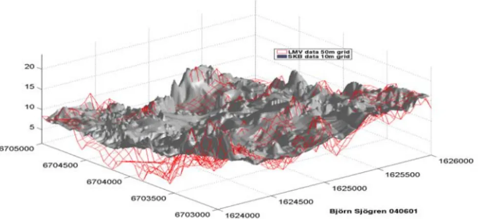
[X,Y,Z]=datagrab(xmin,xmax,ymin,ymax,res,pathname). Observe that datagrab will create an index file. If the content of the directory (containing .G files) is changed, the index file has to be removed in order to make datagrab.m construct a new index file. Elevation data is also provided in a 10x10 m2 grid and is delivered from the SKB site investigation programme. The available format is ASCII and .mat. The area covered by this high-resolution data is ( RT90) X: 6688000-6706000 and Y: 1624000-1643890, i.e. about 18x20 km2. This data is available in Matlab format under
Landuse_CD2/SKB_data/elevationdata/combined_elevationdata.mat. As can be seen in Fig. 2, there is a significant deviation between these two data sets. The reason for this is however not exactly clear.
Certain bathymetry (lake bottom topography) information is available from the “gröna kartan” and this is included in the data-base under
Figure 2. Comparison of topography in the Forsmark area according to the official
50x50 m2 grid used by the National Land Survey of Sweden and results in the 10x10 m2
grid used by SKB.
2.3 Land use
Data on land use is available from the National Land Survey of Sweden in a 25x25 m2 grid. The original ASCII format is quite big, why it has been converted to a more compact Matlab format using the function ●landuse_filemaker.m. The latter format is included in this data-base. The land use is defined in 80 different classes defined in the Excel file SMD_8-bitskoder.xls (available on Landuse_CD1).
A Matlab function ●landuse_merger.m is used to merge landuse files to larger units in the Matlab environment. Landuse_merger.m operates in a similar manner as
datagrab.m, but is somewhat simpler. For instance, it is not possible to set the desired resolution. Observe that the landuse_merger uses an index file. All landuse files plus the index file must be situated in the same directory.
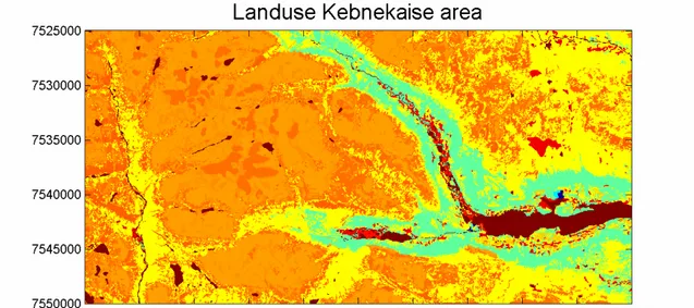
The file ●make_image.m can be used to produce images from the land use data as demonstrated in Fig. 3. One type of colour setting is default, but can be switched to other definitions in the supporting file SMD_8-bitskoder.xls.
Figure 3. Land use data exemplified for the Kebnekaise area.
2.4 Underlying data used for streams and lakes
Geographical extensions of streams, lakes and other wet areas are defined for the area described in section 2.1 and are available in the database (SLU-server \\tala). The data is based on a manual treatment of topographical information obtained from the National Land Survey of Sweden. Similar data is available also at the Swedish Meteorological and Hydrological Institute (SMHI).
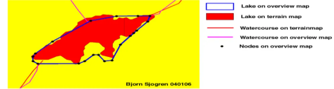
In order to reduce the number of streams and lakes and the associated manual labour, the so called ”Översiktskartan” (the red map, Fig. 4) from the National Land Survey was used in the database. This included 13,899 streams and 8,552 lakes in the area of interest. A stream is delimited by a merging with another stream and, for administrative reasons, also by county (läns-) boundaries. Lakes are any water element that are defined with polygons on the ”Översiktskartan” regardless of their true physical behaviour with respect to stratification or other typicality’s (Fig. 5). Large streams, like Dalälven, are also defined with polygons, such that they become lakes in the database Mires, bogs and other wetlands without a free water surface are not accounted for since
“Översiktskartan” does not contain such information.
The ”Gröna kartan”, which is not used here except for some bathymetric data, makes more distinction between wet areas of various kinds. This, in turn, requires that wetlands are considered in a higher degree in order to provide a continuous stream network (Fig. 4). Regardless of map, the data treatment did consider the need to adjoin water elements so that a continuous stream network was defined.
Figure 4. Comparison of various degree of resolution and definition of water elements between the ”Gröna kartan” and ”Röda kartan” of the National Land Survey of Sweden. The ”Gröna kartan” requires consideration of wetlands in a larger degree to provide a continuous stream network and wet surface area.
Figure 5. Comparison of lake definition on ”Gröna kartan” (red area) and ”Röda kartan” (polygon in blue lines).
As mentioned, there should be a possibility to convert data to the Matlab environment because the groundwater flow simulation is performed in this environment. Particularly important are the boundary conditions for the groundwater flow in terms of connections to surface water volumes such as streams and lakes (see section 5.2). Hence, streams should be defined as vectors and their Strahler order should be defined. The Strahler order is important as a selection criterion in simulation cases of the groundwater flow in which it is necessary to reduce the number of streams that impose boundary conditions in the groundwater model. The stream and lake data have, therefore, been converted to Matlab as described in section 2.5.
2.5 Conversion of data from Shape format to Matlab
All data obtained from the National Land Survey of Sweden is defined in a shape format, i.e. ESRIs compact vector format. The data has been imported and treated in Arcview 3.3.
A shape file (i.e. the .shp file, see below) can be concerted to Matlab by using Arcviews ”Shape to DXF converter” (a separate programme in the start menu). This programme converts the shape file into a DXF-format (a ASCII format). Also ArcToolbox can be used in this purpose. The DXF file can be imported to Matlab by executing the file ●DXF_reader.m (explanation in code).
The shape format consists of three or four files with different endings. The .shp file describes the geographical position, i.e. polygons, vectors or points. This is the file that can be converted to DXF and Matlab format. Another file format, the .dbf file, contains various data, for instance name or a value (like depth) and can be converted to Matlab by the use of Microsoft Excel. Since the procedure of converting .shp to Matlab format does not change the order of the elements, it is easy to connect the information from the .dbf file to the correct feature (polygon, vector or point). Polygons that have been imported to Matlab can be plotted using ● plot_polygon_fr_cell.m.
2.6 Treatment of disjunctive stream network and file type
Lakes and streams should be connected before stream ordering is analysed. The connection is assured by means of the Matlab routine ● build_system.m and the help routine ●connect_wstr_and_lakes.m. The result of the operation is a so called ”struct” variable. A ”struct” contains a “structure array” with specified fields (parameter names) and values associated with the fields, i.e.
s = struct('field1', values1, 'field2', values2, ...)
The value arrays, values1, values2, etc., can be any Matlab element, like cell, string or matrix. A cell is similar to a matrix, but the cell unit can contain any Matlab element. For example, the cell Mycell{1} may contain a matrix and Mycell{2} a string. The struct used to define the stream network characteristics contains 12 parameters (fields) given below. Assume that we have a struct called structname containing N lakes
and K water stretches. This struct will contain the following fields. After Strahler is run, more will be added. Observe the difference between {} and () for cells. {} will give the content of the cell and () will give the cell itself.
outputlake: This is a matrix of size(K,1). If a stream segment discharges into lake, this is specified by the lake index. If outputlake(6) = 14, this means that stream nr 6 flows into lake 14.
inputlake: This is a matrix of size(K,1). If a stream starts at the effluent from a lake, the lake index is specified, see outputlake. wstr_into_lake: This is a matrix of size(N,1). For each lake, the stream index
(the streams are indexed in a similar manner as the lakes) flowing into the lake are specified. If wstr_into_lake(14)=6, this means that lake 14 gets water from stream 6.
wstr_outfrom_lake: This is a matrix of size(N,1). For each lake, the indexes of the stream flowing out of the lake are specified.
outputwstr: This is a matrix of size(K,1). For each stream, the stream index of effluent streams is specified. If outputwstr(4)=22, this means that stream 4 flows into stream 22.
inputwstr: This is a matrix of size(K,1). For each stream, the stream index of influent streams is specified.
roundingfactor: At the connection procedure applied to disjunctive streams it is possible to apply a rounding factor. For instance, roundingfactor = 5 is applied to allow only multiples of 5 meters adjustment. The rounding factor is common to the whole structure. Size(1,1) noinput: This is a matrix of size(K,1). Logical 1 for stream without
tributary stream or lake and zero for other streams. This means that if noinput(56)=1, stream 56 has no tributary.
Nooutput: This is a matrix of size(K,1). Logical 1 for stream that “ends” network, i.e. highest order considered, and zero for all other streams. Since the Ocean is not included here, most of the logical 1 streams are close to the coast.
wstr: This is a cell matrix of size(K,1). This is the coordinates
describing the geographical position of the stream. The first x,y pair describes the point with lowest hydraulic potential and the last the point with the highest. See also “lakes” below. This means that wstr{7} contains a matrix of size (n,2) with n (x,y)-pairs. Then wstr{7}(1,1) is the east coordinate of the point of lowest potential in stream 7 and wstr{7}(1,2) is the north coordinate. plot(structname.wstr{7}(:,1),
structname.wstr{7}(:,2),’b-‘) will plot stream no 7 as a blue line. lakes: This is a cell matrix of size(K,b) where b is the maximum number of
islands. This is the polygon coordinates for all lakes. In fig 5, these
coordinates are represented by black dots. Each row corresponds to a lake. The first cell on the row defines the circumference, the other defines the islands. If lake 8 has 4 islands, lakes{8,1} is the outer boundary,
lakes{8,2} to lakes{8,5}is the islands and cell no 6 to b in row 8 will be empty (the command is empty can help you to determine if there is an island or not). To plot lake 8 as a blue patch, use:
The islands can easily be remover if they are not needed: structname.lakes=structname.lakes(:,1);
stretch: Definition of adjustment stretch required to adjoin stream with lakes in those cases when those elements were disjunctive (see below). The strech is common to the whole structure, just like roundingfactor.
.
Example: The struct vattensystem_m_oar has the field names in the list, while vattensystem_m_oar.wstr is a field containing a cell describing the geographical position of the waterstreches. In this case, vattensystem_m_oar.wstr{5} contains the coordinates of waterstrech number 5. For the lakes, also the islands are included: vattensystem_m_oar.lakes{6,1} contains the polygon describing the circumference of lake number 6. vattensystem_m_oar.lakes{6,2} contains the first island in lake number 6.
The index is the same as the row number. For instance if outputlake(7) =16, this means that the stream at row 7 (i.e. vattensystem_m_oar.wstr{7} flows into lake 16 (i.e. the lake whose circumference is described in vattensystem_m_oar.lakes{16,1}. In total there are 13,899 streams and 8,552 lakes.
Definition of stretch: All streams do not join lake polygons on the national Land Survey
maps even in cases when they should. This makes it impossible to obtain a continuous flow paths. Therefore, a point tangential to the end segments of each stream is utilized in the connection of watestreches and lakes. This is done by linear interpolation of the two end coordinates of the stream. The extra point is situated at the distance stretch from the end of the water stretch. If strech is chosen correctly, the extra point will be situated inside any close by lake polygon boundaries, and it will hereby be possible to determine the flow paths. Strech is defined when build_system.m is run.
In simulation studies and for other analyses, the flow direction is essential information. Such data is derived using the Matlab function ● automatic_waterturnerDEM.m and is included in the ”struct” discussed above, i.e. the coordinates of “wstr” described above are ordered so that the coordinate with the lowest potential comes first.
The topographical data used in the ● automatic_waterturnerDEM.m is not always sufficiently accurate in flat landscapes, due to errors in the elevation data. In such cases, it is possible to use a manual procedure using the function ●manual_waterturner.m. As input for both those routines, the output from build_system.m is needed (also explained in the code). A suggested routine is to first run build_system.m, then
automatic_waterturnerDEM.m to get the flow direction using elevation data. The flow direction can then be adjusted manually using manual_waterturner.m. Observe that manual_waterurner.m is a graphical interface programme and therefore is quite demanding on computational power. Since too large areas may cause problems, it is better to use it on parts of the area, for example Dalarna or Uppland.
2.7 Strahler order
Once the flow directions of streams are known, the Strahler order can readily be calculated. Two functions can be used in this purpose: ● strahler.m or ●strahler2.m. The difference between the two routines is that strahler2.m reduces the stream order with one at bifurcations wile strahler.m does not. Figure 6 shows the ordering principle without bifurcations.
Figure 6. Principal Strahler ordering of a stream network.
2.8 Summary of were to find data in the database
Streams and lakes
Data of streams and lakes are available as a Matlab ”struct” containing the 12 first variables (see section 2.6) and strahler order (based on routine strahler2.m as described in section 2.7) for all streams and lakes. The 13,899 streams are structured in the following order:
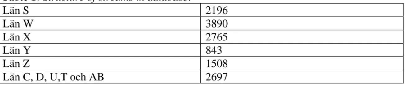
Table 1. Structure of streams in database.
Län S 2196 Län W 3890 Län X 2765 Län Y 843 Län Z 1508 Län C, D, U,T och AB 2697
The data is available under Landuse_CD2/GIS_data/Omradet/. The most extensive struct is final_vattensystem_m_oar.mat. Functions that read and plot the structs are available under the same directory.
Elevation data
Elevation data is available on three CDs in ASCII-format (in the .G format). This is identical to the original LMV data and can be used either with ArcWiew or with Matlab using datagrab.m. The bathymetric data from “Gröna kartan” is available in the file Landuse_CD2/GIS_data/omradet/djupdata_sve.mat.
Landuse
This data is available only in a Matlab format readable with landuse_merger.m (Make sure to copy all landuse data plus the index file to the same directory. See also
landuse_merger.m for instructions) on two CDs. Disc 2 contains also other material than landuse and elevation data, such as Matlab functions and stream network.
SKB data
The SKB elevation data and parts of the GIS data are delivered in a format appropriate to Matlab. The data collected here is available under Landuse_CD2/SKB_data.
Matlab functions
All Matlab functions are available under Landuse_CD2/funktioner/.
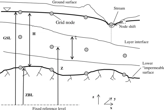
Figure 7. Definition of layered structure used to define grid node system; ZBL is the elevation of bottom layer (m), GSL is the ground surface level (m), H is the water depth (m) and Z is the elevation of node points to be utilised in finite difference formulation (m).
H
ξ
Fixed reference level Ground surface Stream GSL ZBL Layer interface Node shift Z Grid node Lower “impermeable surface x y z
3 Description of groundwater flow model
Chapters 3-5 describe the methodology used to calculate Darcy flow in a three-dimensional groundwater aquifer. A special emphasize is put on providing a
geometrical fit of the grid node system to the free surface and to surface hydrological features which interact with the groundwater, such as streams, lakes and wetlands. The overall objective and limitations of the model framework is described in section 1.3. Infiltration of water through the unsaturated zone is not accounted for in this version of the reporting, but can easily be accounted for. Also an exact fit of the grid to the stream network can be improved and a non-uniform grid can be used.
3.1 Physical background
As will be clear from the subsequent presentation, the groundwater flow problem with a free water surface is non-linear, and consequently there is a need for an iterative
solution procedure and a repeated assembling of the coefficient matrix. The finite difference method simplifies the assembling procedure compared to finite elements and contributes to faster calculations. A problem with the finite difference method in this context, however, is the adaptation of the grid to the free water surface and other features.
The adaptation of the grid net to the free water surface is achieved by defining the groundwater domain in layers (Fig. 7). The layers could be adapted also to geological formations cutting through the groundwater domain. If the layer is comprehended as a two-dimensional structure with a vertical flux to adjacent layers, the continuity equation can be written (Bear, 1979)
∂nρξ
∂t + ∇ ⋅ (ρVξ)+ρqZ+ ∆ξ/ 2-ρqZ− ∆ξ/ 2 = Q (2)
in which bold face type denote a vector quantity, V is the Darcy flow velocity (m/s), i.e. product of pore water velocity and porosity, the Nabla operator ∇ = (∂/∂x,∂/∂y) (in two dimensions), n is the porosity, ρ is the water density (kg/m3), ξ is the layer thickness
(m), q is vertical flow velocity across layer interfaces (m/s) and Q is a source or sink term (kg/(m2 s)), such as infiltration in the uppermost layer.
Equation (2) and the subsequent numerical approximations introduced in this section imply that the (x,y)-components of the velocity are not horizontal. This problem could be remedied if the (x,y)-components of the velocity in the leaning layers are
recalculated in terms of a 3D orthogonal coordinate system. Hence, the coordinates (x,y) should be considered as a local system and this x,y-plane generally has different slope in various grid nodes. This implies that the distances between nodes depend on their position as well as the slope of layers. In the finite difference method proposed below, the distances between nodes within the layers are calculated without
consideration of the slope of the layers. This simplification is appropriate if the slope of the water surface is relatively small.
At the uppermost layers, ξ is delimited by the water surface and may change over time. However, at the internal layers the time derivative of ξ can normally be neglected. In geohydraulics, the porosity is normally referred to as the storativity (denoted by S). For both open and porous media flows, the depth-averaged form of the momentum equation in two dimensions (in the horizontal plane) can generally be stated as (Chow, 1959) 1 g ∂V ∂t + V ⋅ ∇V +∇( p ρg+ Z) = − f 8R V | V | g (3)
where p = pressure (Pa), g = acceleration due to gravity (m/s2), h = water depth (m), z = elevation of bottom of flow in relation to an arbitrary (but constant) datum plane (m), f = Darcy Weisbach friction factor (-) and R= size of typical flow channels (in fractures, canals, granular material) (m). For groundwater flow, the inertia terms of the left-hand side of (3) can normally be neglected also for flow in relatively fast flow in coarse gravel. For similar cases, for which the velocity head can be neglected, Eqn. (2) can be written for stationary flow
∇( p ρg+ Z) = − f 8R V | V | g (4)
If we also have Reynolds numbers, Re = V R / ν smaller than 10 the friction factor is inversely proportional to Re, f = a/Re, where a = a coefficient and ν = kinematic viscosity (m2/s) (Bear, 1980). This implies that Eqn. (4) can be rewritten as
V = K ∇( p
ρg+ Z) (5)
where the hydraulic conductivity K = (8 R2 g)/(a f ν), can be expressed also in terms of a friction factor F = 1/K.
Finally, if (5) is combined with the continuity equation for stationary, incompressible flow we have ∇ Kξ∇ p ρg+ Z ⎛ ⎝ ⎜ ⎞ ⎠ ⎟ ⎛ ⎝ ⎜ ⎞ ⎠ ⎟ − qZ+ ∆ξ/ 2+ qZ− ∆ξ/ 2= −Q (6)
3.2 Numerical methods
DiscretisationThe routine matsolve.m solves Eqn. (6) for the hydraulic potential h = p/(ρ g) + Z (m). By applying the central finite differences to the (x,y)-components of Eqn. (6), the equation becomes
Tj,i+1+ Tj,i
(xj,i+1− xj,i−1)(xj,i+1− xj,i)hj,i+1−
− Tj,i+1+ Tj,i
(xj,i+1− xj,i−1)(xj,i+1− xj,i)+
Tj,i+ Tj,i−1
(xj,i+1− xj,i−1)(xj,i− xj,i−1) ⎡ ⎣ ⎢ ⎤ ⎦ ⎥ hj,i+ Tj,i+ Tj,i− i
(xj,i+1− xj,i−1)(xj,i− xj,i−1)hj,i−1+
Tj+1,i+ Tj,i
(yj+1,i− yj−1,i)(yj+1,i− yj,i)hj+1,i−
− Tj+1,i+ Tj,i
(yj+1,i− yj−1,i)(yj+1,i− yj,i)+
Tj+ Tj−1
(yj+1,i− yj−1,i)(yj,i− yj−1,i) ⎡ ⎣ ⎢ ⎤ ⎦ ⎥ hj,i+ Tj,i+ Tj−1,i
(yj+1,i− yj−1,i)(yj,i− yj−1,i)hj−1,i− qZ+ ∆ξ/ 2+ qZ− ∆ξ/ 2= −Q (7)
where the hydraulic transmissivity of each layer T = ξ K, i denotes node number in x-direction (column in e.g. code and Numb) and j denotes y-x-direction (row in e.g. code and Numb).
In case of constant distances between the nodes (7) simplifies to
(Tj,i+1+ Tj,i)
2∆X2 hj,i+1−
Tj,i+1+ 2Tj,i+ Tj,i−1
[
]
2∆X2 +
Tj+1,i+ 2Tj,i+ Tj−1,i
[
]
2∆Y2 ⎡ ⎣ ⎢ ⎢ ⎤ ⎦ ⎥ ⎥ hj,i+ +(Tj,i+ Tj,i− i) 2∆X2 hj,i−1+ (Tj+1,i+ Tj,i) 2∆Y2 hj+1,i+ (Tj,i+ Tj−1,i) 2∆Y2 hj−1,i− qZ+ ∆ξ / 2+ qZ− ∆ξ / 2= −Q (8) If it is assumed that the grid nodes, except those in the upper most and the lowest layer, are placed (vertically) in the middle of each layer (as shown in Fig. 7). Grid nodes in the two layers that are handled differently are located at the ground surface level and at the impermeable bottom level. The thickness of these two layers differs are half of that used in the other layers. This means that for a specific location (x,y), the vertical distance between the grid points is the same. The vertical fluxes in Eqn (8) can be expressed (e.g. Freeze and Cherry, 1979):k j i k j i k j i k j i k j i Z K K h h q ijk , , , , 1 , , 1 , , , , 2 / 1 , , 2 ξ ξ ξ − − = + + ∆ + + (9) qZ− ∆ξ/ 2= 2 hi , j ,k − hi, j,k−1 ξi, j,k Ki, j,k − ξi, j,k−1 Ki, j,k−1 (10)
where hi,j,k+1 is the overlying layer and hi,j,k-1 is the underlying layer. Similar three
dimensional variables are used for most of the properties of Fig. 7. Eqns. (9) – (10) can be derived by expressing the vertical velocity between two layers using two expressions based on the hydraulic potential of an imaginary node point introduced between the layers and which is eliminated between the two expressions.
In addition to the q-terms, the vertical fluxes appear also in the (x,y)-components of the velocity. This is because of the slope of the grid layers and will have consequences for the calculation of velocity components in an orthogonal coordinate system and to the particle tracking.
[
]
[
]
[
]
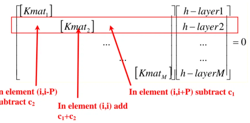
0 ... ... 2 1 ... ... 2 1 = ⎥ ⎥ ⎥ ⎥ ⎥ ⎥ ⎦ ⎤ ⎢ ⎢ ⎢ ⎢ ⎢ ⎢ ⎣ ⎡ − − − ⎥ ⎥ ⎥ ⎥ ⎥ ⎥ ⎦ ⎤ ⎢ ⎢ ⎢ ⎢ ⎢ ⎢ ⎣ ⎡ layerM h layer h layer h Kmat Kmat Kmat MFigure 8. Structure of equation system, where Kmat indicates a PxP sub-matrix of each
layer and red text indicates contribution of vertical fluxes related to element (i,i) and connected nodes. Since each layer has equal node structure, the connected nodes in the vertical directions are enumerated (i,i+P) and (i,i-P).
Assembling of coefficient matrix
The structure of the simultaneous equation system as defined by (8) for the entire grid node system can be illustrated as in Fig 2.
In Fig. 8, Kmat = sub-matrix for each layer that contains only (two-dimensional) (x,y)-components and the vertical fluxes are represented by adding contributions along the main diagonal (i,i) and to elements corresponding to connecting nodes, i.e. (i,i+P) and (i,i-P) as shown in Fig 2, where P is the total number of nodes included in the two-dimensional (layered) calculation domain (see section 5.1). If the nodes are placed in the middle of each layer and (9) and (10) are substituted in (8), the c-coefficients of Fig.8 can be rewritten on a form:
c1= 0.5 /(Zi, j,k+1− Zi, j,k) 1/Ki, j,k+1+ 1/Ki, j,k (11) c1= 0.5 /(Zi, j,k − Zi, j,k−1) 1/Ki, j,k+ 1/Ki, j,k−1 (12)
Enumeration of nodes and corresponding structure of the individual Kmat sub-matrices are discussed in section 5.1. Because each layer have the same structure and (x,y)-coordinates of the nodes, each sub-matrix will be identical with exception for boundary conditions in all three directions. The five-node approximation also leads to a generally
In element (i,i+P) subtract c1
In element (i,i-P)
subtract c2 In element (i,i) add
banded structure of the sub-matrix, but which is interrupted by roughness of boundaries in the (x,y)-directions.
The (c1 +c2) represent the influx to each layer and is added for each term along the main
diagonal (although only indicated for one row in Fig. 8) except at the uppermost and lowermost layers which are treated specially.
Boundary conditions
To recognise a von Neuman condition at a boundary node, we replace Eqn. (7) with
h = known value (13)
This condition is applicable when node points coincide with surface water of a known hydraulic potential (Fig. 7) but can also utilized when the groundwater surface are assumed to follow the ground surface. Treatment of the exact node location in relation to stream geometry is discussed in section 5.2.
Implementation of a Dirichlet condition need to consider the stationary form of Eqn. (2): ∇(V ξ) = 0. In a discretised form this becomes (Vx ξ)i+1/2-(Vx ξ)i-1/2+(Vy ξ)j+1/2-(Vy
ξ)j-1/2 = 0. The "half-node-locations” are introduced because when V is expressed
according to Eqn. (5) and ξ is formulated as central finite differences, only the node values are used to represent ξ. For instance, if the flux in terms of θ = V ξ is known at i+1/2, the corresponding expression to Eqn. (8) with constant discretisation segments ∆X and ∆Y becomes
θj,i+1/ 2 ∆X − Tj,i+ Tj,i−1 2∆X2 hj,i+ Tj,i+ Tj,i− i 2∆X2 hj,i−1+ Tj+1,i+ Tj,i 2∆Y2 hj+1,i− − Tj+1,i+ Tj,i 2∆Y2 + Tj,i+ Tj−1,i 2∆Y2 ⎡ ⎣ ⎢ ⎤ ⎦ ⎥ hj,i+ Tj,i+ Tj−1,i 2∆Y2 hj−1,i− qZ+ ∆ξ/ 2+ qZ− ∆ξ/ 2= 0 (14) The implication of this approach is that the flux across the boundary in any of the directions i+1/2, …j-1/2 can be explicitly expressed. For a closed boundary, the flux is zero.
Iterative solution algorithm
Because the transmissivities of (8) depends on the water depth/hydraulic potential, the coefficient matrix depends on the solution, i.e. the problem is linear. The non-linearity requires an iterative solution procedure where the coefficient matrix is
gradually updated. This iteration is preceded by defining the grid node system based on assumed start values of water depth. The iteration includes the following steps:
- Assemble equation system based on "old" values of water depth in coefficient matrix
- Solve system
- Let water depth equal hydraulic potential in uppermost layer of nodes - Define new grid net
- Error is calculated based on change in water depth between iterations - Calculation is continued as long as error exceeds a certain limit
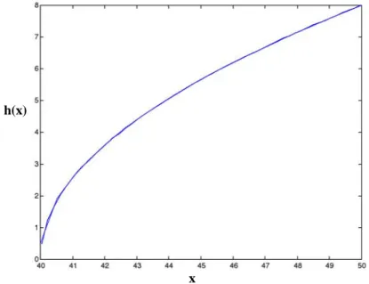
3.3 Verification of numerical accuracy using closed-form solutions
A simple verification of the numerical accuracy of the solution to (8) was performed based on a one-dimensional solution. This comparison was based on the special case; a rectangular single layer, a Dirichlet condition at two of the opposite (shorter) boundaries and no-flow conditions on the transversal boundaries. Basically the problem is one-dimensional with the closed-form solution
h2(x)= (h22− h12)x− x0
L− x0 + h1
2
(15)
where x is the coordinate in the flow direction, h1 is the boundary condition at x=x0 and
h2 is the boundary condition at x = L. The numerical solution is obtained for h2 and
subsequently transformed to h. As can be seen in Fig. 9 the deviation between the numerical and the closed-form solutions is marginal.
The other closed-form solution used to evaluate the calculation programme is that of a sink and a source placed in an infinite two-dimensional space and equal transmissivity (cf. Fig. 10), which means that (8) is in the form of Laplace equation. The solution to this problem is readily obtained in cylindrical coordinates for one source at the time. The final solution in terms of velocity components is obtained by superimposing the two source solutions in Cartesian coordinates on the form of
vx= S cos arctan x y ⎛ ⎝ ⎜ ⎞ ⎠ ⎟ ⎡ ⎣ ⎢ ⎤ ⎦ ⎥ 1 x2+ y2 − cos arctan x− L y ⎛ ⎝ ⎜ ⎞ ⎠ ⎟ ⎡ ⎣ ⎢ ⎤ ⎦ ⎥ 1 (x− L)2+ y2 ⎧ ⎨ ⎩ ⎫ ⎬ ⎭ (16a) vy= S sin arctan x y ⎛ ⎝ ⎜ ⎞ ⎠ ⎟ ⎡ ⎣ ⎢ ⎤ ⎦ ⎥ 1 x2+ y2 − sin arctan x− L y ⎛ ⎝ ⎜ ⎞ ⎠ ⎟ ⎡ ⎣ ⎢ ⎤ ⎦ ⎥ 1 (x− L)2+ y2 ⎧ ⎨ ⎩ ⎫ ⎬ ⎭ (16b)
where the origin is placed in the source point (in this example), S = strength of sources and L is the distance between the source and the sink.
Figure 9. Comparison of one-dimensional solution according to numerical model (solid curve) and closed-form solution (dashed curve). Note that the two curves coincide.
Figure 10. Numerical solution to the problem with a source and a sink of equal
strength. Potential surface is shown on the left-hand side and velocity vectors to the right.
x h(x)
The numerical solution is obtained for non-flow conditions at the boundaries and the problem formulation is consequently only an approximation of that stated for the closed-form solution. Therefore, the error was evaluated only at node points on node points in a square between the sink and the source. The mean error of the relative velocity deviation was 0.6% in one test.
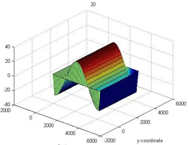
Also a three dimensional calculation test was performed, where 35 layers were used to describe a 4100x4100x1000 m box. The surface was given a specified head distribution, formed as a uniformed wave in the form of
C kx h
h= msin( )+ (16)
where hm is the half amplitude of the head variation, k is the wave number, x is the
coordinate parallel to the surface and C is the mean value of the head distribution. For this given head distribution at the surface there is an exact analytical solution for the head distribution at any given depth (Packman and Bencala, 2000):
[
kd kz kz]
Ckx h
h= msin( )tanh( b)sinh( )+cosh( ) + (17)
Where db is the total depth of the box, z is the coordinate perpendicular to the surface.
The solution for layer 20 is shown in figure 11.
Figure 11. Analytical solution of the head distribution at layer 20 (of 35) for a
calculation problem with a wave formed head distribution at surface.
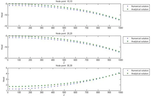
In figure 12 a numerical solution for the corresponding layer is shown and figure 13 shows a comparison between the numerical and the analytical solution. In figure 13 the accuracy dependence of depth are presented at three different node points in the
Figure 12. Numerical solution of the head distribution at layer 20 (of 35) for problem with a wave formed head distribution at surface.
Figure 13. Comparison between analytical and numerical solution at three different
node points in the horizontal plane. For each point, the differences in terms of head due to Z are presented.
4 Simple user guide for computer codes
This section contains a simple user guide and a description of programme features. Functioning of programme and definition of programme variables are described in section 5. Variables are marked with bold face type the first time they appear in their description.
In summary, the programme calculates the 3D distribution of hydraulic potential or water surface elevation given locations of the boundary and statements of boundary conditions. Most statements are provided in in data files that are loaded into the Matlab working space, but some statements need to be done directly in the executable files. All required files are listed in Appendix 1. This version of the programme does not consider infiltration of water, which can be added as a source term in the uppermost layer, nor an exact fitting of the grid to surface water elements.
4.1 Indata
Before the programme is run, the problem needs to be defined in the following indata files (unformated text/ASCII-files):
- koord: In this file the geometry of the calculation domain is defined. The real
boundary is approximated by a limited number of straight lines that encloses the real domain (see section 5.1 for details).
- BC1: This file states the type of boundary condition on each of the lines used to define the calculation domain. The programme can handle a given flow (e.g. zero) or a known potential. Details are given in section 5.2.
- BC2x and BC2y: These files state numerical values of the flux components or a given value of the potential. Details are given in section 5.2.
- BC3: In this file it is possible to set boundary conditions to individual nodes used in the calculation. In order to be able to set these conditions, it is necessary to run the first programme called "flownet.m". When this programme has been run, the grid enumeration can be displayed and the specific node be identified. See section 5.2 for details.
- K-values: The hydraulic conductivity or flow resistance can be given explicitly in individual node points. This is done by either loading a matrix called F in the beginning of matsolve.m. If the hydraulic conductivity is constant (homogeneous condition), this can be set directly in the matslove.m code. Details are given in sections 3.2 and 5.3.
- Surface.txt: This file states which type of treatment should be applied to nodes in the top-layer. At this stage, the programme can handle a given hydraulic potential. Source term for infiltration could be added. Details are given in section 5.2. - BC.txt: Specifies boundary conditions for the top-layer. At this stage, only the
hydraulic potential can be stated to represent contact with surface water of known water level. Details are given in section 5.2.
- ZBL.txt: Specifies The elevation of the lower impermeable surface of the calculation domain. Details are given in section 5.1.
- GSL.txt: Specifies ground surface elevation that can be used in some plots and used as starting values for the water surface in the iterative solution algorithm.
- Hydraulic conductivities are set in the file matsolve.m. In this version, a constant hydraulic conductivity is applied. Se section 5.3 for more details.
Numerical variables may need to be set in the programme files (the matlab.m-files) before they are executed. The functioning of the programme and the different variables are described in section 5. The most essential variables that need to be set are:
- NX: Is set in "flownet.m". Defines the number of segments used in the help grid (see section 5.2).
- NY: Is set in "flownet.m". Defines the number of segments used in the help grid (see section 5.2).
- M: Is set in “matsolve.m”. Defines the number of 2D-layers.
- transx: Is set in "flownet.m". Governs the placement of the help grid in relation to the approximated domain (see section 5.2).
- transy: Is set in "flownet.m". Governs the placement of the help grid in relation to the approximated domain (see section 5.2).
- fact: Is set in "flownet.m". Governs the placement of the help grid in relation to the approximated domain (see section 5.2).
4.2 Executing the programmes
Start by executing "flownet.m", which will lead to the generation of a 2D calculation grid that can be applied to each layer. After this has been run, it may be necessary to modify the grid generation by changing parameters directly in the Matlab codes and execute flownet.m repeatedly. Analysis of the generated grid is needed in order to write the indata file BC3. In BC3, it is possible to assign boundary conditions to individual node points. See section 5.1 for details.
Run “BCpoints.m”, but only if needed. This file loads BC3 and defines boundary conditions for individual node points along the circumference of the 2D-layers. In the current version of the programme, all layers are defined with the same conditions. See section 5.2 for details.
Run “matsolve.m”. This programme loads all in-data files defines the 3D-conditions (see section 4.1), assembles the necessary matrices and solves the equation system described in sections 3.2 and 5.3 The hydraulic potential of the uppermost layer is contained in the matrix "res". See section 5.3 for details.
The result can be analysed by running “velocities.m” and "partrack.m". At this point, these files can only handle a single layer. "velocities.m" calculates velocity vectors and provides a plot of these vectors. "partrack.m" performs a particle tracking and calculates certain characteristics, such as residence times of particles. The residence time
distribution can also be analysed in more detail by running the code “PDFs.m”.
4.3 Forsmark calculation example
This example presents a calculation of the hydraulic head in a 75x75 km area (figure 14) that covers the Forsmark site area. The elevation data of the area was imported from the database as described in chapter 2.2 and then used as “BC.txt” (see 4.1). The
resolution of the data is one node point every 625th meter, which means that the area includes 121x121 node points in every horizontal layer. The number of layers was set to be 10 and the total number of node points was 146410. The lower, impermeable
Figure 14. Elevation data from the Forsmark area.
The results of executing “flownet.m” and “matsolve.m” (see 4.2) are given in figure 15-18, where the head distributions in three different layers are presented. Figure 15 shows the bottom layer (layer 1) 5000 m below seepage, figure 16 is a view of layer 7 which are located between 1618 and 1668 m below seepage, figure 17 is a view of layer 9 which are located between 491 and 557 m below seepage and the head distribution at ground surface level is presented in figure 18.
Figure 16. Head distribution in layer 7 of 10, 1618-1668 m below seepage.
Figure 18. Head distribution in layer 10 of 10, at ground surface level.
5 Description of codes for groundwater flow
5.1 Definition of boundary geometry and grid net
The boundary position in the (x,y)-directions is defined in the text file "koord" (unformated). The first column of "koord" contains x-coordinates of points along the boundary and the second column contains corresponding y-coordinates:
64.81 35.19 70.37 46.30 68.52 64.81 …
In order to be able to construct a suitable grid net, the boundary can be translated in x- and y-directions using the variables "transx" and "transy" directly in the file
0 50 100 150 200 250 300 350 0 50 100 150 200 250 300 350
Figure 18. Approximation of real boundary using discrete points on the boundary.
0 50 100 150 200 250 300 350 0 50 100 150 200 250 300 350
Figure 19. Help grid net (small points and circles) in a 31 x 31 matrix and calculation
grid (only circles). Number of segments in help grid is defined by NX and NY.
φ [m] ζ [m] Point 1: [64.81+transx,35.19+transy] Help grid: XX(1:NX+1) and YY(1+NY+1) Calculation grid Approximated boundary Line 1 φ [m] ζ [m]
Figure. 20. Colour coding of grid points (each square corresponds to one grid node) with respect to their geometrical appearance. This information is stored in "code". The colour code is explained in the text.
On top of the approximated boundary, a help grid is defined with the vectors XX and YY. The numbers of segments in x- and y-direction are defined by NX and NYdirectly in "flownet.m" (the number of points is NX+1 and NY+1). One reason for introducing the help grid is that the Matlab plot commands require rectangular fields (matrix arguments). The variable "fact" is used directly in "flownet.m" to enlarge the help grid (in percentage of the size of the approximation domain) as can be seen in Fig. 19. "flownet.m" uses equidistant node separation in x- and y-directions.
The file "flownet.m" analyses which help grid points are inside the approximated domain and assigns a numerical value to the matrix code(NX+1,NY+1) for each point included and zero for each point excluded from the calculation grid (Figs. 19 and 20). If there is a point in the help grid closer to the approximated boundary than that inside the domain on the same row, this node is included in the calculation grid.
Since the assemblage of the simultaneous equation system depends on the geometrical feature of the calculation grid at the boundary, the matrix "code" makes use of the following coding of the node points in the help grid (Figs. 20 and 21):
0 = Dark red in Fig. 21: not included node 1 = Light red in Fig. 21: node included in grid
2 = Orange in Fig. 21: boundary condition, node on vertical node-line with domain on the right hand side (three nodes in a column)
3 = boundary condition, node on vertical node-line with domain on the left hand side (three nodes in a column)
4 = Light yellow (beige) in Fig. 21: boundary condition, node on horizontal node-line with domain on higher-y-side (lower row!) (three nodes on a horizontal line)
5 = Yellow in Fig. 21: boundary condition, node on horizontal node-line with domain on lower-y-side (three nodes on a horizontal line)
6 = Lightest blue in Fig. 21: boundary condition, corner node - lower-y-side (upper row!) and left
7 = Middle blue No. 1 in Fig. 21: boundary condition, corner node - lower-y-side and right
8 = Middle blue No. 2 in Fig. 21: boundary condition, corner node - higher-y-side and left
9 = Dark blue in Fig. 21: boundary condition, corner node - higher-y-side and right
code = 2 code = 3 code = 4 code = 5
code = 6 code = 7 code = 8 code = 9
Figure 21. Coding of grid nodes on the boundar(marked with star) with respect to
structure of neighbouring nodes. This information is stored in "code".
Nodes with only one neighbouring node (as in Fig. 19 on row 7 and column 8) are omitted from the final help grid.
Note that increasing the y-coordinate corresponds to higher rows in code(row,column). Hence, if code is displayed in the command window of Matlab, a number "9" will appear on corner nodes on the lower right side. Fig. 20 shows the result of the following command series in "flownet":
surf(XX,YY,-code)
xlabel('x-coordinate'),ylabel('y-coordinate') AZ = -17.5; EL = 90; view(AZ,EL)
Further, the calculation nodes are numbered in the order from first row and fist column, first row and second column, … last row and last column in the matrix "Numb". This information is used when the coefficient matrix is assembled.
All layers are the same and treated in the manner described above. The number of layers are specified in the file “matsolve.m”, whereas the location of the impermeable bottom surface and ground surface are defined in the indata files ZBL(NX+1,NY+1) and GSL(NX+1,NY+1). These files are loaded by the Matlab-file “matsolve.m”. Layers are enumerated from the bottom to top, resulting in Layer No. M at the top.
5.2 Definition of boundary conditions
The boundary points in the (x,y)-directions are coded with respect to their boundary condition. All layers are equally defined in the current version of the programme.
The load file "BC1" is used to code the lines in the approximation domain. The following coding is used
1. von Neuman = specified value on water surface elevation 2. Dirichlet = specified flow in (m2/s) conditions
The actual definition of a Dirichlet condition is a known value of the derivative of the unknown function, but since the derivative of the hydraulic potential is linearly
proportional to flow (in the Darcy case, see section 3), the condition is stated in terms of flow. BC1 should be arranged in a single column. In BC2x and BC2y, numerical values are assigned for the magnitude of the condition and sign for direction in the coordinate system XX and YY. Each file should be arranged as a single column.
A situation could be to have a known potential at the in- and outflow section and zero flow across the boundary in between. Hence, if BC1 states a "2" for line 1 (at first row in the single column of BC1) we know that line 1 is associated with a flow condition. Further, by assigning "0" in the first row of both BC2x and BC2y we know that the x- and y-components of the flow is zero. A known leakage through the boundary in terms of V h (see section 2.2) should be stated in units [m3/(s m)] in BC2x and BC2y. The sign of the flux should be defined in terms of the coordinate system, not e.g. direction in relation to the boundary. For instance, an inflow is positive on the "left-hand side" of the domain, whereas an inflow is negative on the "right-hand side".
A possibility is that the inflow section is given by a line defined in BC1 (the position of the line is given in "koord"). Hence, BC1 should state a "2" at the row corresponding to the line and the corresponding flux components in BC2x and BC2y.
The in- and outflow in the (x,y)-directions can be defined through the lines defined in koord by stating a known hydraulic potential in these sections. Place a "1" in BC1 at the row corresponding to the certain line and the value of the hydraulic potential in BC2x. In this case of a von Neuman condition, the content of in the file BC2y on the row corresponding to the certain line is ignored. Any numerical value can be (and also must be) stated on this row in BC2y.
Figure 22. Coding of boundary points with respect to their boundary condition, von Neuman and Dirichlet, respectively. This information is stored in "code2". Dark blue implies a zero flux and light green implies a known potential. The matrices code3x and code3y contain numerical values of the boundary conditions.
Figure 24. Equipotential lines as plotted by the routine "matsolve.m".
The type of boundary condition is stored in "code2(NX+1,NY+1)" using the same indices as for "code" and "Numb". The numerical values of the grid points are stored in code3x and code3y.
A suitable way of defining the in- and outflow section in the (x,y)-direction is to define the hydraulic potential in individual node points. After "flownet.m" has been run, you can analyse the location of the calculation points in the XX(1:NX+1)-YY(1:NY+1)-system. One way to see the location where the in- and outflow should be defined is to use the plot of the matrix "code" that is provided by the "flownet.m" programme (cf. Fig. 20). It is also possible to display "code" in the command window row-by-row by writing "code(row,:)" followed by return. When the right position has been identified the following information should be written in the file BC3:
Four columns define: Node row and column number (in help grid), BC type and a numerical value defining the boundary condition. This information is written on each single row for each node used in the definition. For the coding exemplified in Fig. 22, the BC3 file looks like this:
9 8 1 2 29 5 1 8
For a comparison of the column and row numbers, please confer Fig. 19 in which the rows and columns are easy to count.
The boundary condition along the lower domain surface is implicitly taken as no flow in the current version of the programme. The boundary condition at the upper surface is stated in the indata files BC.txt(NX+1,NY+1) and surface.txt(NX+1,NY+1). The file surface.txt states which type of treatment should be applied to nodes in the top-layer. If