02:37 Theoretical and Numerical Evaluation of the MTC Noise Estimate in 2-D 2-group Heterogeneous Systems

SKI Report 02:37

Research

Theoretical and Numerical Evaluation

of the MTC Noise Estimate in 2-D 2-group

Heterogeneous Systems

Christophe Demazière

January 2002

SKI PERSPECTIVE

How this project has contributed to SKI’s research goals

The overall goals for SKI research are:

• to give a basis for SKI ’s supervision

• to maintain and develop the competence and research capacity within areas which are important to reactor safety

• to contribute directly to the Swedish safety work.

The project has contributed to the research goal of giving a basis for SKI’s supervision by developing a non-intrusive method for determination of the moderator temperature coefficient (MTC) in pressurized water reactors (PWRs). The MTC is an important safety parameter which has to be measured twice during a fuel cycle in PWRs.

Furthermore, the project has also contributed to the strategical research goal of competence and research capacity by building up competence within the

Department of Reactor Physics at Chalmers University of Technology regarding reactor physics, reactor dynamics and noise diagnostics.

Project information:

Project manager: Ninos Garis, Department of Reactor Technology, SKI

Project number: 14.5-011142-01261

SKI Report 02:37

Research

Theoretical and Numerical Evaluation

of the MTC Noise Estimate in 2-D 2-group

Heterogeneous Systems

Christophe Demazière

Chalmers University of Technology

Department of Reactor Pysics

412 96 Göteborg

Sweden

January 2002

This report concerns a study which has been conducted for the Swedish Nuclear

Table of contents

Summary/Sammanfattning 5

1. Introduction 6

2.1. Description of the core 8

2.2. Description of the static core simulator 11

2.3. Description of the adjoint core simulator 17

2.4. Description of the noise simulator 19

4. Results 38

4.1. Specification of the noise source 38

4.2. Calculated MTC noise estimators 39

5. Conclusions 43

6. References 44

7. Nomenclature 45

2. Calculation of the static flux, the adjoint flux, and the reac-tor transfer function

7

3. Derivation of the MTC noise estimators for 2-D 2-group heterogeneous systems

25

3.1. Calculation of the reactivity noise in multigroup perturbation theory

25 3.2. Calibration of the noise simulator results to the

SIMULATE-3 results

32 3.3. Derivation of the MTC noise estimators in the D

2-group approximation

Summary

The effect of a heterogeneous distribution of the temperature noise on the MTC estimation by noise analysis is investigated. This investigation relies on the 2-group diffusion theory, and all the calculations are performed in a 2-D realistic heterogeneous core. It is shown, similarly to the 1-D case, that the main reason of the MTC underestimation by noise analysis compared to its design-predicted value lies with the fact that the temperature noise might not be homogeneous in the core, and therefore using the local temperature noise in the MTC noise estimation gives erroneous results. A new MTC estimator, which was previously proposed for 1-D 1-group homogeneous cases and which is able to take this heterogeneity into account, was extended to D 2-group heterogeneous cases. It was proven that this new estimator is always able to give a correct MTC estimation with an accuracy of 4%. This small discrepancy comes from the fact that the reactor does not behave in a point-kinetic way, contrary to the assumptions used in the noise estimators. This discrepancy is however quite small.

One quantitative result of the present work is a measure of the underestimation of the traditional method as a function of the correlation length of the temperature fluctuations. It is found that the underestimation is larger in 2-D for the same correlation length as in the 1-D case. An underestimation with a factor 5 in the present model is obtained with a radial correlation length of 150 cm. Comparisons with measurements will be possible to make in measurements to be performed in Ringhals.

Sammanfattning

Inverkan av den inhomogena rumsfördelningen av temperaturfluktuationerna för

bestämningen av MTK (moderatortemperaturkoefficienten) med brusanalys har

undersökts och rapporterats. Undersökningen i detta arbete är baserad på tvågrupps-diffusionsteori. Alla beräkningar har gjorts i en 2-D realistisk reaktorhärd. Liksom i en tidigare undersökning i 1-D finner vi, att den huvudsakliga anledningen till att den traditionella brusmetoden underskattar moderatortemperturkoefficienten är inhomogeni-teten av temperaturfluktuationerna, varför användning av ett lokalt värde på temperaturfluktuationerna ger felaktigt resultat. Den nya så kallade estimatorn, det vill säga en algoritm för bestämning av MTK, som nyligen har föreslagits och testats av oss i 1-D, har nu utvidgats till att omfatta 2-D 2-gruppsteorin. Undersökningarna som rapporteras här visar, att den nya estimatorn skattar den verkliga temperaturkoefficienten med en noggrannhet på 4 %. Det jämförelsevis lilla felet härrör från reaktorresponsens avvikelse från punktkinetik, eftersom även den nya algoritmen förutsätter att reaktorns beteende är punktkinetiskt. Denna avvikelse är dock ganska liten.

Ett resultat av föreliggande arbete är det kvantitativa sambandet mellan underskattning av MTK med den traditionella brusmetoden och korrelationslängden av temperaturfluktuationerna. Vi fann att underskattningen i 2-D vid en viss korrela-tionslängd är större än i 1-D. En underskattning med en faktor 5 erhålls i föreliggande arbete vid en korrelationslängd på 150 cm. Jämförelse med mätningar från Ringhals kommer att göras.

1. Introduction

There have been many attempts in the past few years to monitor the Moderator Temper-ature Coefficient of reactivity (MTC) by noise analysis in Pressurized Water Reactors (PWRs). In these experimental investigations, the MTC is inferred from the signals deliv-ered by an in-core neutron detector and a core-exit thermocouple located in the same fuel channel or in two neighbouring fuel channels. The measured neutron noise and tempera-ture noise contain some information about the dynamics of the reactor, and in particular on the MTC, while the reactor is still at its normal and steady-state operating conditions. This noise technique is therefore very well suited to monitor the MTC at full power, since unlike the traditional measurement techniques such as the boron dilution method or the control rod swap, the reactor does not need to be perturbed.

Due to the reactor transient that the traditional measurement techniques induce and their relatively large uncertainty on the MTC estimation, it was considered that measuring the at-power MTC could be avoided, since core calculations were believed to give an accurate estimation of the at-power MTC. Thus a more and more common practice was to measure the MTC at Beginning of Cycle (BOC) and Hot Zero Power (HZP), a measurement which is accurate and relatively easy to perform, and then to rely completely on core calculations for the variation of the MTC with burnup. Nevertheless, this at-power MTC calculation was never benchmarked. Furthermore, with the use of high burnup or Mixed Oxide (MOX) fuel assemblies, the MTC might become positive at BOC. For the high burnup fuel bundles, the positive contribution is due to the high boron concentration necessary to compensate for the reactivity excess of the fuel. For the MOX fuel, the positive contribution is due to the 0.3 eV resonance of Pu-239. Therefore being able to monitor the MTC throughout the whole fuel cycle could become again of great interest in the near future. The noise technique is very interesting in this respect, since such a measurement can be carried out at any time during the fuel cycle without disturbing the reactor operation.

Nevertheless, all the experimental work revealed that the MTC was systematically underestimated by a factor of two to five compared to its design-predicted value (see (Demazière, 2000) for a complete list of References in this matter). This underestimation was found to be constant during a fuel cycle, and even between several fuel cycles as long as the same pair of detectors is used for the estimation. Many factors could influence the accuracy of the MTC noise estimation. Several of them were investigated in the past. Although correction factors were proposed accordingly, either the correction factors are negligible, or they cannot be estimated easily in practice. A new aspect which could explain the underestimation of the noise analysis technique was considered recently (Pázsit et al, 2000), (Demazière and Pázsit, 2002), namely the spatially heterogeneous distribution of the temperature noise throughout the core. It was found that the main reason of the MTC underestimation might be due to the fact that the temperature noise was measured in one-point of the reactor, whereas the MTC relies on the core average temperature noise and that this temperature noise is most likely strongly spatially heterogeneous. The spatial inhomogeneity of the temperature noise has actually been confirmed in recent measurements (Demazière et al, 2000a). On the other hand, the resulting deviation of the reactor response from point-kinetics, an approximation on which the MTC noise estimator relies, was found to be negligible with respect to the

MTC estimation. Consequently, one new MTC noise estimator that allows taking the spatial structure of the temperature noise into account was proposed by us recently and was proven to give an accurate MTC estimation (Pázsit et al, 2000), (Demazière and Pázsit, 2002).

This above mentioned study only investigated 1-D one-group homogeneous systems in the diffusion approximation. In this report, the investigation is extended to 2-D two-group heterogeneous systems in the diffusion approximation. The main goals of the work were as follows:

1. To extend the definition of the average temperature to a 2-group case (this is not triv-ial); with the definition, give a new biased estimator for the determination of the MTC which is only biased with the deviation of the reactor response from point kinetics;

2. To elaborate calculational methods for the investigation of the performance of the tra-ditional and the new estimators in 2-D 2-group theory;

3. To verify that the qualitative conclusions of the 1-D investigation regarding the reason of the underestimation of the MTC by the traditional method are similar in 2-D; 4. To investigate quantitatively the dependence of the magnitude of the MTC

underesti-mation by the traditional noise method as a function of the correlation length of the temperature fluctuations.

The first part of the report is devoted to the models used in the simulation. The second part deals with the derivation of the MTC noise estimate for 2-D 2-group heterogeneous systems, which is slightly different from the 1-D 1-group homogeneous systems. Finally, the results of the calculations are presented in more detail. It was found that the new MTC estimator was always able to give a correct MTC estimation. This finding further confirms that the deviation of the reactor response from point-kinetics does not play a significant role for the MTC estimation, whereas the spatial inhomogeneity of the temperature noise has a very decisive effect. The usual MTC noise estimator was found to underestimate the MTC more significantly than for the 1-D one-group homogeneous cases.

A nomenclature explaining all the abbreviations used in this report can be found at the end (see Section 7).

2. Calculation of the static flux, the adjoint

flux, and the reactor transfer function

The traditional MTC noise estimator, i.e. the one that was used in all the experimental work so far, is based on the measurement of the temperature noise, the induced neutron noise, and the static flux. As will be described in more detail in Section 3, the new MTC noise estimator in addition relies also on the adjoint flux, which is needed for the calcula-tion of the core average temperature noise. Consequently, a static core simulator, an ad-joint core simulator, and a noise simulator are required for the theoretical investigation of the MTC estimation by noise analysis.

2.1. Description of the core

A realistic heterogeneous system was chosen for this investigation, namely the Ringhals-4 PWR with the operational conditions as of May 5th, 1999. At that date, the at-power MTC was measured by using the boron dilution method. This measurement was per-formed a few months before the expected EOC of the fuel cycle 16, more precisely at a core average burnup of 8.767 GWd/tHM. This measurement, which is required by the Swedish safety authorities, is intended to verify that the magnitude of the MTC will not exceed a given value for the remaining part of the cycle, therefore preventing from the consequences of a reactivity transient, induced by an incidental cooldown event. During this measurement, the MTC was found to be equal to -58.12 pcm/ C 11.68 pcm/ C (Demazière et al, 2000b). The MTC was also directly calculated by SIMULATE-3 (Um-barger and DiGiovine, 1992) by simply increasing the coolant inlet temperature by +5 F (2.78 C), all the other parameters remaining constant. It was found that:

(1) This value will be considered in the following as the reference and target value1 of the MTC for the noise analysis technique.

As will be seen in the following, the 2-D 2-group material data and the point-kinetic parameters of the core are required for the calculation of the induced neutron noise via the noise simulator. Furthermore, the static flux and the adjoint flux are also required in this 2-D and 2-group derivation. The static flux is needed for the neutron noise simulator itself and the MTC estimation in the noise analysis technique, whereas the adjoint flux is used (together with the static flux) for calculating the core average temperature noise. One could use SIMULATE-3 to provide all these quantities. Nevertheless, the static and adjoint fluxes need to be recalculated via a simulator using the same spatial discretisation scheme as the one used in the neutron noise simulator. Otherwise, using the static and adjoint fluxes directly from SIMULATE-3 is equivalent to make the system non-critical2. Another simpler approach could have been to modify the cross-sections in each node (while keeping the static and adjoint fluxes from SIMULATE-3) so that the balance equations were fulfilled for the same spatial discretisation scheme as the one used in the noise simulator. This approach was tested in the present case but showed that some cross-sections became negative.

Hence, the 2-group cross-sections provided by SIMULATE-3 for each node were homogenised from 3-D to 2-D in order to be used by the 2-D simulators. The homogenization was naturally carried out by using the static fluxes as weighting functions so that the reaction rates were preserved:

1. Only the ratios between the MTC noise estimators and the actual value of the MTC are investi-gated in this study. The MTC is only evaluated in relative terms, therefore the actual MTC value does not really matter since the MTC noise estimators can be scaled to any value (see Section 3.2).

2. The static and adjoint fluxes (and their associated eigenvalues) are nevertheless used in the static and adjoint core simulators as a starting guess in the power iteration method.

° ± °

° °

(2)

and

(3)

with having a broad meaning, i.e. being , , , or . All the other

symbols have their usual meaning with representing the volume of the node

(I,J,K). G is the group index ( for the fast group, and for the thermal group). Similarly, the adjoint fluxes were homogenised as follows:

(4)

Although this way of averaging the material data and the fluxes preserves the reaction rates, the 2-D system which is thus obtained will have a much higher eigenvalue than the 3-D system since the leakage in the axial direction was eliminated (a 2-D system is in fact assumed to be infinite in the third direction). Therefore, if one wants results compatible with the actual 3-D core, one has to take the axial leakage into account in the 2-D system. This can be done by increasing the absorption cross-section in each group by an artificial leakage cross-section in the same group, which allows having the correct leakage rate when multiplied by the corresponding group flux. For that purpose, one needs to evaluate the axial leakage rate in each node for the 3-D system. Since this leakage rate is not given by SIMULATE-3, the finite difference scheme is used instead (this finite difference scheme is also used in the static core simulator, the adjoint core simulator, and the neutron noise simulator). In the “box-scheme” approximation, this reads as (Nakamura, 1977): (5) X S_{G I J, ,} XS_{G I J K, , ,} φ_{G I J K, , ,} V_{I J K, ,} K

∑

φ_{G I J K, , ,} V_{I J K, ,} K

∑

---= φ_{G I J, ,} φ_{G I J K, , ,} V_{I J K, ,} K

∑

V_{I J K, ,} K

∑

---= X S_G D_G Σ_{a G,} Σ_rem νΣ_{f G,} V_{I J K, ,} G = 1 G = 2 φ_{G I J}+_{, ,} φ_{G I J K}+_{, , ,} V_{I J K, ,} K

∑

V_{I J K, ,} K

∑

---=

leakage rate in group G and node I J K( , , ) 1 ∆z ---[a_{G I J K}z_{, , ,} φ_{G I J K, , ,} +b_{G I J K}z_{, , ,} φ_{G I J K, , , +1}+c_{G I J K}z_{, , ,} φ_{G I J K, , , –1}] – LR_{G I J K, , ,} = =

with the coefficients , , and given by the following Table 1:

The corresponding “leakage” cross-sections are thus given by:

(6)

so that the absorption cross-sections are modified in the following way:

(7) Then the homogenization is carried out as described before, i.e. according to Eq. (2).

Concerning the noise calculation described in Section 2.4, one has to select also the frequency at which the evaluation has to be performed. In the MTC investigation by noise analysis, it is common practice to determine the MTC in the frequency range 0.1 -1.0 Hz. The lower frequency bound allows using in the MTC noise estimators the zero-power reactor transfer function instead of the at-zero-power reactor transfer function (which is unknown since it contains the MTC). This substitution is valid because the cut-off frequency corresponding to the heat transfer between coolant and fuel is lower than 0.1 Hz. The upper bound is due to the damping of the temperature fluctuations travelling from the in-core neutron detector to the core-exit thermocouple, if the traditional noise Table 1: Coupling coefficients in the z direction.

if the node K-1 does not exist 0 if the nodes K-1 and K+1 both exist if the node K+1 does not exist 0 a_{G I J K}z_{, , ,} b_{G I J K}z_{, , ,} c_{G I J K}z_{, , ,} a_{G I J K}z_{, , ,} b_{G I J K}z_{, , ,} c_{G I J K}z_{, , ,} 2 D_{G I J K, , ,} D_{G I J K, , , +1} ∆z D( _{G I J K, , ,} +D_{G I, , ,J K+1}) ---2 D_{G I J K, , ,} ∆z ---+ 2D_{G I J K, , ,} D_{G I J K, , , +1} ∆z D( _{G I J K, , ,} +D_{G I J K, , , +1}) ---– 2 D_{G I J K, , ,} D_{G I J K, , , +1} ∆z D( _{G I J K, , ,} +D_{G I J K, , , +1}) ---2D_{G I J, ,} D_{G I J K, , , –1} ∆z D( _{G I J K, , ,} +D_{G I J K, , , –1}) ---+ 2D_{G I J K, , ,} D_{G I J K, , , +1} ∆z D( _{G I J K, , ,} +D_{G I J K, , , +1}) ---– 2 DG I J K, , , DG I J K, , , –1 ∆z D( _{G I J K, , ,} +D_{G I J K, , , –1}) ---– 2 D_{G I J K, , ,} ∆z ---2 D_{G I J K, , ,} D_{G I J K, , , –1} ∆z D( _{G I J K, , ,} +D_{G I J K, , , –1}) ---+ 2 D_{G I J K, , ,} D_{G I J K, , , –1} ∆z D( _{G I J K, , ,} +D_{G I J K, , , –1}) ---– L_{G I J K, , ,} LRG I J K, , , φ_{G I J K, , ,} ---– = Σ_{a G I J K}*_{, , , , Σ} a G I J K, , , , +LG I J K, , , =

estimator is used. In our case, the axial direction is disregarded, so that the upper limit has no significance. It was therefore decided to perform all the noise calculations at that frequency, i.e. 1 Hz.

2.2. Description of the static core simulator

As described previously, the static flux is needed in this theoretical investigation for three main reasons. First of all, the static flux is required for the calculation of the neutron noise, since the noise source strength is always proportional to the static flux (see Section 2.4). Second, the static flux is used in the MTC noise estimators, since only the neutron noise relative to its mean value is of interest (see Section 3). Finally, the static flux is used to-gether with the adjoint flux to calculate the coolant average temperature noise throughout the core (see Section 3).

In the two-group diffusion approximation, the static flux is the solution of the following matrix equation:

(8)

where

(9)

(10)

This system of equations has to be spatially discretised. Finite differences were used for that task, and more precisely the so-called “box-scheme” (more information regarding this specific point can be found in (Pázsit et al, 2000) and (Pázsit et al, 2001), where the discretisation scheme was extensively explained):

(11) D r( )∇2+Σ( )r [ ] φ1( )r φ₂( )r × = 0 D r( ) D1( )r 0 0 D₂( )r = Σ( )r νΣ_{f 1,} ( )r k_eff ---–Σ_{a 1,} ( )r –Σ_rem( )r νΣf 2, ( )r k_eff ---Σ_rem( )r –Σ_{a 2,} ( )r = 1 ∆x⋅∆y --- D_G( )∇r 2φ_G( )r dr I J, (

∫

) a_{G I J}x_{, ,} φ_{G I J, ,} +b_{G I J}x_{, ,} φ_{G I, +1,J} +c_{G I J}x_{, ,} φ_{G I, –1,J} ( ) ∆x ---– a_{G I J}y_{, ,} φ_{G I J, ,} +b_{G I J}y_{, ,} φ_{G I J, , +1}+c_{G I J}y_{, ,} φ_{G I J, , –1} ( ) ∆y ---– =

with the different coefficients , , , , , and sum-marised in Table 2 and Table 3 for the x and y directions respectively.

Table 2: Coupling coefficients in the x direction.

if the node I-1 does not exist 0 if the nodes I-1 and I+1 both exist if the node I+1 does not exist 0

Table 3: Coupling coefficients in the y direction.

if the node J-1 does not exist 0 if the nodes J-1 and J+1 both exist a_{G I J}x_{, ,} a_{G I J}y_{, ,} b_{G I J}x_{, ,} b_{G I J}y_{, ,} c_{G I J}x_{, ,} c_{G I J}y_{, ,} a_{G I J K}x_{, , ,} b_{G I J K}x_{, , ,} c_{G I J K}x_{, , ,} 2 D_{G I J, ,} D_{G I, +1 J,} ∆x D( _{G I J, ,} +D_{G I, +1 J,} ) ---2 D_{G I J, ,} ∆x ---+ 2D_{G I J, ,} D_{G I, +1 J,} ∆x D( _{G I J, ,} +D_{G I, +1 J,} ) ---– 2D_{G I J, ,} D_{G I, +1 J,} ∆x D( _{G I J, ,} +D_{G I, +1 J,} ) ---2 D_{G I J, ,} D_{G I 1, – ,J} ∆x D( _{G I J, ,} +D_{G I 1, – ,J}) ---+ 2D_{G I J, ,} D_{G I, +1 J,} ∆x D( _{G I J, ,} +D_{G I, +1 J,} ) ---– 2 DG I J, , DG I 1, – ,J ∆x D( _{G I J, ,} +D_{G I 1, – ,J}) ---– 2D_{G I J, ,} ∆x ---2 D_{G I J, ,} D_{G I 1, – ,J} ∆x D( _{G I J, ,} +D_{G I 1, – ,J}) ---+ 2 D_{G I J, ,} D_{G I 1, – ,J} ∆x D( _{G I J, ,} +D_{G I 1, – ,J}) ---– a_{G I J K}y_{, , ,} b_{G I J K}y_{, , ,} c_{G I J K}y_{, , ,} 2 D_{G I J, ,} D_{G I J, , +1} ∆y D( _{G I J, ,} +D_{G I J, , +1}) ---2 D_{G I J, ,} ∆y ---+ 2D_{G I J, ,} D_{G I J, , +1} ∆y D( _{G I J, ,} +D_{G I J, , +1}) ---– 2 D_{G I J, ,} D_{G I J, , +1} ∆y D( _{G I J, ,} +D_{G I J, , +1}) ---2 D_{G I J, ,} D_{G I J, , –1} ∆y D( _{G I J, ,} +D_{G I J, , –1}) ---+ 2D_{G I J, ,} D_{G I J, , +1} ∆y D( _{G I J, ,} +D_{G I J, , +1}) ---– 2 DG I J, , DG I J, , –1 ∆y D( _{G I J, ,} +D_{G I J, , –1}) ---–

The matrix equation given by Eq. (8) has to be used to determine both the two-group fluxes and the eigenvalue. This can be done via the so-called outer iteration that can be summarised as follows. If one rewrites Eqs. (8) - (10) as:

(12)

with

(13)

(14)

(15)

then the flux and the eigenvalue can be searched for by using an iterative scheme. In the present study, the power iteration method was chosen for its simplicity and its relative ef-ficiency (Bell and Glasstone, 1970), (Nakamura, 1977). In such a method, the flux and the eigenvalue are given by the following expressions:

(16) and (17) if the node J+1 does not exist 0 Table 3: Coupling coefficients in the y direction.

a_{G I J K}y_{, , ,} b_{G I J K}y_{, , ,} c_{G I J K}y_{, , ,} 2 D_{G I J, ,} ∆y ---2 D_{G I J, ,} D_{G I J, , –1} ∆y D( _{G I J, ,} +D_{G I J, , –1}) ---+ 2 D_{G I J, ,} D_{G I J, , –1} ∆y D( _{G I J, ,} +D_{G I J, , –1}) ---– M r( ) φ× ( )r 1 k_eff ---F r( ) φ× ( )r = M r( ) Σa 1, ( ) Σr rem( )r D1( )∇r 2 – + 0 Σ_rem( )r – Σ_{a 2,} ( )r –D₂( )∇r 2 = F r( ) νΣf 1, ( )r νΣf 2, ( )r 0 0 = φ( )r φ1( )r φ₂( )r = φ( )n ( )r M–1( )r 1 k_eff(n–1) ---F r( ) φ× (n–1)( )r × = k_eff( )n F r( ) φ n ( ) r ( ) × F r( ) φ× (n–1)( )r ---×k_eff(n–1) =

where (n) represents the iteration number. The starting point of this method is an initial

guess for and . In this study, the values given by SIMULATE-3 were

cho-sen3. Then, a new flux distribution is calculated via Eq. (16), and subsequently a new ei-genvalue is estimated via Eq. (17). This procedure is repeated until some convergence criteria regarding both the neutron flux and the eigenvalue are fulfilled. Then the results have to be scaled since Eq. (8) is a homogeneous equation. The scaling is required for comparison purposes between the static core simulator and SIMULATE-3 (the MTC es-timated theoretically via the noise technique is independent of this scaling, see Section 3). The scaling factor is calculated so that the power level corresponds to the one given by SIMULATE-3 in the axially condensed reactor:

(18)

where and are the energy release per fast and thermal fission respectively. This static core simulator was then benchmarked against SIMULATE-3. In such a benchmark, the cross-sections used in the 2-D simulator were obviously obtained directly from the 3-D core modelled in SIMULATE-3 without any modification of the absorption cross-sections (which would have been necessary to take the leakage in the axial direction into account, as described previously (see Section 2.1)). Such a cross-section adjustment would have made the axially condensed systems significantly different with respect to the flux calculation. It is therefore expected that the eigenvalue given by the static core simulator (2-D system) will be significantly larger than the one given by SIMULATE-3 (3-D system).

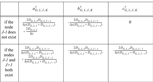
The results of the benchmarking are given in Figs. 1 and 2. The peaks observed in Fig. 1 correspond to the reflector peaks, i.e. an increase of the thermal flux in the reflector region, and are also observed in the SIMULATE-3 results. Furthermore, the agreement between the static core simulator and SIMULATE-3 is very good in the fuel zone. The discrepancy is nevertheless relatively significant in the reflector zone for two main reasons. First of all, the discretisation scheme used in the static core simulator, i.e. the finite difference scheme, is known to give poor results when there are large flux gradients, such as for instance in the reflector region and close to this region. SIMULATE-3 uses a nodal diffusion model, which gives much more accurate results in such cases. Another difference between the two modelling is the number of nodes used in the calculation. In SIMULATE-3, the core is described via a 32x32 lattice, whereas the static core simulator uses a 64x64 lattice. In order to compare the results of the two calculations, the SIMULATE-3 results were simply expanded on the 64x64 grid without any interpolation, i.e. the results are spatially homogeneous on each 2x2 node. Consequently, a reflector “bundle” is actually described by 2x2 nodes in the static core simulator, whereas it is described by only 1x1 node in SIMULATE-3. Since the static

3. For the flux, the axially condensed flux given by SIMULATE-3 is actually used.

φ( )0

r

( ) k_eff( )0

κ₁( )φr ₁( ) κr + ₂( )φr ₂( )r

[ ]dr

fuel

∫

_{static core simulator}

κ₁( )φr ₁( ) κr + ₂( )φr ₂( )r

[ ]dr

fuel

∫

_SIMULATE-3 =

0.5 1 1.5 2 2.5 3 3.5 10 20 30 40 50 60 10 20 30 40 50 60 0 0.5 1 1.5 2 2.5 3 3.5 4 x 1014 J coordinate (1) I coordinate (1) φ 1 (n.cm −2 .s − 1) 0 1 2 3 4 5 6 7 10 20 30 40 50 60 10 20 30 40 50 60 0 1 2 3 4 5 6 7 8 x 1013 J coordinate (1) I coordinate (1) φ2 (n.cm − 2.s − 1)

Figure 1: Static flux calculations provided by the static core simulator in the benchmark case (the fast flux is given in the upper figure, and the thermal flux is given in the lower figure)

−80 −60 −40 −20 0 20 40 60 10 20 30 40 50 60 10 20 30 40 50 60 (φ 1−φ1,ref)/φ1,ref (%) J coordinate (1) I coordinate (1) −80 −60 −40 −20 0 20 40 60 10 20 30 40 50 60 10 20 30 40 50 60 (φ₂−φ_2,ref)/φ_2,ref (%) J coordinate (1) I coordinate (1)

Figure 2: Relative difference in the static flux calculations between the static core simulator and SIMULATE-3 in the benchmark case, with SIMULATE-3 being considered as the reference case; the comparison of the fast flux is given in the upper figure, and the comparison of the thermal flux is given in the lower one

flux is assumed to vanish at the core boundary, big discrepancies are thus expected in the reflector region. Concerning the eigenvalue calculation, the static core simulator gives a value of 1.00332, whereas SIMULATE-3 gives a value of 0.99998. This discrepancy was expected since the static core simulator represents a 2-D system in which the axial leakage was eliminated, whereas SIMULATE-3 represents an actual 3-D system.

2.3. Description of the adjoint core simulator

As mentioned previously, the adjoint flux, together with the static flux, is needed in this theoretical investigation for the calculation of the coolant average temperature noise throughout the core (see Section 3).

In the two-group diffusion approximation, the adjoint flux is solution of the following matrix equation:

(19)

where is given by Eq. (9) and where is the adjoint of , i.e. its transpose:

(20)

The spatial discretisation is carried out as before, i.e. by using the finite differences and the so-called “box-scheme”:

(21)

with the different coefficients , , , , , and given

previously (see Table 2 and Table 3).

The matrix equation given by Eq. (19) has to be used to determine both the two-group adjoint fluxes and the eigenvalue. In principle the eigenvalue of the direct problem should be equal to the eigenvalue of the adjoint problem. Nevertheless, due the discretisation scheme used in the calculations, it is not granted that these two eigenvalues

D r( )∇2+Σ+( )r [ ] φ1 + r ( ) φ₂+ r ( ) × = 0 D r( ) Σ+( )r Σ( )r Σ+( )r νΣ_{f 1,} ( )r k_eff ---–Σ_{a 1,} ( )r –Σ_rem( )r Σ_rem( )r νΣ_{f 2,} ( )r k_eff --- –Σ_{a 2,} ( )r = 1 ∆x⋅∆y --- D_G( )∇r 2φ_G+( )r dr I J, (

∫

) a_{G I J}x_{, ,} φ_{G I J}+_{, ,} +b_{G I J}x_{, ,} φ_{G I}+_{, +1,J} +c_{G I J}x_{, ,} φ_{G I}+_{, –1,J} ( ) ∆x ---– a_{G I J}y_{, ,} φ_{G I J}+_{, ,} +b_{G I J}y_{, ,} φ_{G I J}+_{, , +1}+c_{G I J}y_{, ,} φ_{G I J}+_{, , –1} ( ) ∆y ---– = a_{G I J}x_{, ,} a_{G I J}y_{, ,} b_{G I J}x_{, ,} b_{G I J}y_{, ,} c_{G I J}x_{, ,} c_{G I J}y_{, ,}

are still identical in the discretised problem. If the two simulators, i.e. the static and the adjoint ones, are consistent, then the two numerical eigenvalues should be very close to each other (as will be seen in the following, the two eigenvalues are actually identical). Therefore the eigenvalue calculation has to be performed simultaneously with the flux calculation, in order to verify that the difference between the two eigenvalues is negligible. This can be done as before via the so-called outer iteration that can be summarised as follows. If one rewrites Eqs. (19) and (20) as:

(22)

where and are the adjoint of and respectively, i.e. their

trans-pose:

(23)

(24)

and

(25)

then the flux and the eigenvalue can be searched for by using an iterative scheme. By us-ing as before the power iteration method, the flux and the eigenvalue are given by the fol-lowing expressions:

(26)

and

(27)

where (n) represents the iteration number. The starting point of this method is an initial

guess for and . In this study, the values given by SIMULATE-3 were

cho-sen4. Then, a new adjoint flux distribution is calculated via Eq. (26), and subsequently a new eigenvalue is estimated via Eq. (27). This procedure is repeated until some

conver-M+( ) φr × +( )r 1 k_eff+ ---F+( ) φr × +( )r = M+( )r F+( )r M r( ) F r( ) M+( )r Σa 1, ( ) Σr rem( )r D1( )∇r 2 – + –Σ_rem( )r 0 Σ_{a 2,} ( )r –D₂( )∇r 2 = F+( )r νΣf 1, ( )r 0 νΣ_{f 2,} ( )r 0 = φ+ r ( ) φ1 + r ( ) φ₂+ r ( ) = φ+ n( ) r ( ) M+ 1– ( )r 1 k_eff+ n( –1) ---F+( ) φr × + n( –1)( )r × = k_eff+ n( ) F + r ( ) φ+ n( ) r ( ) × F+( ) φr × + n( –1)( )r ---×k_eff+ n( –1) = φ+ 0( ) r ( ) k_eff+ 0( )

gence criteria regarding both the neutron flux and the eigenvalue are fulfilled. Then the results have to be scaled since Eq. (19) is a homogeneous equation. The scaling is required for comparison purposes between the adjoint core simulator and SIMULATE-3 (the MTC estimated theoretically via the noise technique is independent of this scaling, see Section 3). The scaling factor is calculated so that the volume integral of the fast adjoint flux is equal to unity:

(28)

where V_core is the volume of the core (without reflector, i.e. only the fuel region).

This adjoint core simulator was then benchmarked against SIMULATE-3. In such a benchmark, the cross-sections used in the 2-D simulator were once again obtained directly from the 3-D core modelled in SIMULATE-3 without any modification of the absorption cross-sections. It is therefore expected that the eigenvalue given by the adjoint core simulator (2-D system) will be significantly larger than the one given by SIMULATE-3 (3-D system).

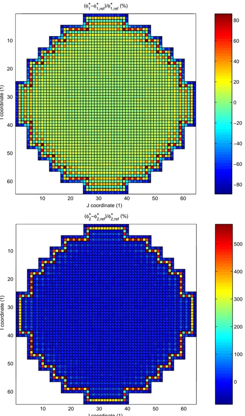
The results of the benchmarking are given in Figs. 3 and 4. As can be seen in these figures, the agreement between the adjoint core simulator and SIMULATE-3 is very good in the fuel zone, whereas the discrepancy is significant in the reflector zone. The same reasons as the ones presented for the static core simulator could explain this discrepancy, i.e. the difference in the spatial discretisation schemes between SIMULATE-3 and the adjoint core simulator, and the different number of nodes used for the calculations. Concerning the eigenvalue calculation, the adjoint core simulator gives a value of 1.00332, whereas SIMULATE-3 gives a value of 0.99998 for . These values are identical to the ones given by the static direct calculations. The discrepancy between the SIMULATE-3 and the adjoint core simulator results was expected since the adjoint core simulator represents a 2-D system in which the axial leakage was eliminated, whereas SIMULATE-3 represents an actual 3-D system.

2.4. Description of the noise simulator

The neutron noise simulator was extensively described in (Pázsit et al, 2000) and (Pázsit et al, 2001). In the following, only the main characteristics of this neutron noise simulator are recalled.

The neutron noise simulator is able to calculate the spatial distribution of the neutron noise induced by any given spatially distributed or localised noise sources. Several types of noise sources can be simultaneously investigated, i.e. a perturbation of the macroscopic absorption cross-section (fast and/or thermal), and/or a perturbation of the macroscopic removal cross-section, and/or a perturbation of the macroscopic fission cross-section (fast and/or thermal). The neutron noise simulator is able to model the noise sources of the “absorber of variable strength” type (the so-called reactor

1 V_core --- φ₁+( )r dr core

∫

1 = k_eff+

0.2 0.4 0.6 0.8 1 1.2 10 20 30 40 50 60 10 20 30 40 50 60 0 0.2 0.4 0.6 0.8 1 1.2 1.4 J coordinate (1) I coordinate (1) φ + (1)1 0.2 0.4 0.6 0.8 1 1.2 1.4 1.6 1.8 10 20 30 40 50 60 10 20 30 40 50 60 0 0.5 1 1.5 2 J coordinate (1) I coordinate (1) φ2 (1)

Figure 3: Adjoint flux calculations provided by the static core simulator in the benchmark case (the fast flux is given in the upper figure, and the thermal flux is given in the lower figure)

−80 −60 −40 −20 0 20 40 60 80 10 20 30 40 50 60 10 20 30 40 50 60 (φ+ 1−φ + 1,ref)/φ + 1,ref (%) J coordinate (1) I coordinate (1) 0 100 200 300 400 500 10 20 30 40 50 60 10 20 30 40 50 60 (φ+ 2−φ + 2,ref)/φ + 2,ref (%) J coordinate (1) I coordinate (1)

Figure 4: Relative difference in the adjoint flux calculations between the adjoint core simulator and SIMULATE-3 in the benchmark case, with SIMULATE-3 being considered as the reference case; the comparison of the fast adjoint is given in the upper figure, and the comparison of the thermal adjoint is given in the lower one

oscillator). The simulator cannot model noise sources of the “moving absorber” type. Furthermore, the calculations are directly performed in the frequency domain.

If the noise source is a point source of unit strength, the neutron noise simulator

actually estimates the 2-D 2-group discretised Green’s function , the

index representing the fast and thermal groups respectively. More specifically, these transfer functions give the flux noise in and at a frequency

induced by a unit cross-section noise source located at at the same frequency.

In the linear two-group diffusion theory, the neutron noise can be expressed as a solution of the following matrix equation:

(29)

where the different matrices/vector are given as:

(30)

(31)

(32)

(33)

and the different coefficients are defined as:

(34) (35) G_XS→i(r r, ,′ ω) i = 1 2, δφ_i r f = ω⁄2π δXS = 1 r′ D r( )∇2+Σ(r,ω) [ ] δφ1(r,ω) δφ₂(r,ω) × φrem( )δΣr _rem(r,ω) φa( )r δΣa 1, (r,ω) δΣ_{a 2,} (r,ω) +φf(r,ω) δνΣ_{f 1,} (r,ω) δνΣ_{f 2,} (r,ω) + = Σ(r,ω) –Σ1(r,ω) νΣf 2, (r,ω) Σ_rem( )r –Σ_{a 2,} (r,ω) = φrem( )r φ₁( )r φ – ₁( )r = φa( )r φ1( )r 0 0 φ₂( )r = φf(r,ω) φ1( )r 1 iωβ_eff iω λ+ ---–     – φ₂( )r 1 iωβeff iω λ+ ---–     – 0 0 = Σ₁(r,ω) Σ_{a 1,} ( )r iω v₁ --- Σ_rem( ) νΣr _{f 1,} ( )r 1 iωβeff iω λ+ ---–     – + + = νΣ_{f 2,} (r,ω) νΣ_{f 2,} ( )r 1 iωβeff iω λ+ ---–     =

(36)

The matrix is identical to the one given by Eq. (9).

The spatial discretisation is carried out as before, i.e. by using the finite differences and the so-called “box-scheme”:

(37)

with the different coefficients , , , , , and given

previously (see Table 2 and Table 3).

Unlike the calculation of the static flux and the adjoint flux, the equation giving the neutron noise, i.e. Eq. (29), is not a homogeneous equation, but represents a source

problem. Consequently, the discretised form of the matrix can be

directly inverted, and the flux noise calculated accordingly.

Even if Eq. (29) was written for any kind of noise sources, only one type will be investigated in the MTC study. In order to determine which macroscopic cross-section is the most sensitive to the coolant temperature, two SIMULATE-3 calculations were run: the first one at the nominal operating conditions corresponding to the operational point described previously, i.e. on May 5th, 1999, and the second one for the same burnup but with a core inlet temperature increased by +5 F (2.78 C). For this second calculation, the fuel temperature was kept equal to the one estimated during the first calculation, and so were the main fission products (promethium, samarium, iodine, and xenon). Three quantities are then studied (all the 0-D parameters are directly obtained from SIMULATE-3):

• The relative variation (in percent) of each macroscopic cross-section defined as:

(38)

• The relative variation (in percent) of the corresponding reaction rate defined as:

(39)

where G is the group index associated with the cross-section variation which is studied;

Σ_{a 2,} (r,ω) Σ_{a 2,} ( )r iω v₂ ---+ = D r( ) 1 ∆x⋅∆y --- D_G( )∇r 2δφ_G(r,ω)dr I J, (

∫

) a_{G I J}x_{, ,} δφ_{G I J, ,} ( )ω +b_{G I J}x_{, ,} δφ_{G I, +1,J}( )ω +c_{G I J}x_{, ,} δφ_{G I, –1,J}( )ω ( ) ∆x ---– a_{G I J}y_{, ,} δφ_{G I J, ,} ( )ω +b_{G I J}y_{, ,} δφ_{G I J, , +1}( )ω +c_{G I J}y_{, ,} δφ_{G I J, , –1}( )ω ( ) ∆y ---– = a_{G I J}x_{, ,} a_{G I J}y_{, ,} b_{G I J}x_{, ,} b_{G I J}y_{, ,} c_{G I J}x_{, ,} c_{G I J}y_{, ,} D r( )∇2+φ(r,ω) [ ] ° ° ∆X S_0-D X S0-D T, in+5– X S0-D T, in X S_{0-D T,} in ---×100 = ∆RR_0-D X S0-D T, in+5×φG 0-D T, , in+5– X S0-D T, in×φG 0-D T, , in X S_{0-D T,} in×φG 0-D T, , in ---×100 =

• The corresponding reactivity variation (in pcm) for each different type of cross-sec-tion given as:

(40)

where the effective multiplication factor, at a given core inlet temperature, is evaluated according to the following formula:

(41)

All the symbols in Eq. (41) have their usual meaning. When evaluating Eq. (41), the effect of the change of each cross-section was studied separately, i.e. was estimated by using the value of this specific cross-section at , all the other cross-sections taken at .

The results are summarised in the following Table 4. As can be seen, the cross-section that has the largest reactivity effect is the macroscopic removal cross-cross-section. Therefore in the following, the noise source will be assumed to be a macroscopic removal cross-section noise, i.e. the noise simulator will calculate the transfer function from the macroscopic removal cross-section noise source to the induced neutron noise.

The neutron noise simulator was already benchmarked previously during Stage 7 of the SKI project (Pázsit et al, 2001). In the following, only the case of a macroscopic removal cross-section noise is presented. The layout of the core in this benchmark is representative of the Swedish BWR Forsmark-1. The core was assumed to be a two-region system (fuel + reflector), in which each two-region was spatially homogeneous. The material constants, the point-kinetic parameters and the flux data were obtained from a Table 4: Effect of a variationof the core inlet temperature (+5 F) oneach of the macroscopic cross-sections (%) -0.94 -0.15 -0.21 -0.17 -0.13 (%) -0.21 0.59 -0.21 0.57 -0.14 (pcm) -414 60 207 -35 -105 ∆ρ keff T, in+5–keff T, in k_{eff T} in , 2 ---×105 = k_eff νΣ_{f 2 0-D, ,} νΣ_{f 1 0-D, ,} φ1 0-D, φ_{2 0-D,} ---× + Σ_{a 2 0-D, ,} ---Σ_{rem 0-D,} Σ_{a 1 0-D, ,} +Σ_{rem 0-D,} --- 1 1 _Σ D1 0-D, a 1 0-D, , +Σrem 0-D, ---×B_{g 1 0-D}2_{, ,} + --- 1 1 _ΣD2 0-D, a 2 0-D, , ---×B2_{g 2 0-D, ,} + ---× × × = k_{eff T} in+5 , T_in+5 T_in ° X S_0-D Σ_{rem 0-D,} Σ_{a 1 0-D, ,} Σ_{a 2 0-D, ,} νΣ_{f 1 0-D, ,} νΣ_{f 2 0-D, ,} ∆X S_0-D ∆RR_0-D ∆ρ

generic General Electric BWR/6. At that time, the flux was not recalculated with a dicretisation scheme compatible with the finite difference scheme, so that the macroscopic cross-sections were slightly adjusted in each node in order to fulfil the balance equations in each node with respect to the finite difference scheme (as written in (Pázsit et al, 2001), this adjustment was only noticeable close to and in the reflector region). The noise source was located in the middle of the core. Since the core was roughly homogeneous, an analytical solution could be estimated and was used as a reference solution. The results of this benchmark are presented in Figs. 5 and 6. Since the noise source was located in the middle of the core, the results are rotational-invariant around the z-axis crossing the core centre. Therefore only the radial dependence of the fluxes is plotted in the Figures.

It can be noticed that the agreement between the numerical solution and the analytical one is very good for both the magnitude and the phase of the induced neutron noise. Since the noise simulator calculates a spatially-averaged flux noise over each node, the analytical solution was also averaged over each node, so that both solutions could be directly compared. The first point of the numerical solution (from the core centre) represents therefore the flux noise in the node where the noise source is located. The analytical solution gives obviously a different solution in this node, and thus the first point of the analytical solution was systematically disregarded. Finally, due to the cross-section adjustment, which is noticeable only around the reflector region, the accuracy close to the reflector deteriorates slightly, but remains still acceptable. Another reason explaining this discrepancy lies with the fact that the analytical solution does not take any reflector into account.

3. Derivation of the MTC noise estimators for

2-D 2-group heterogeneous systems

According to the recent American Standard (ANSI, 1997), the MTC is defined as the var-iation of reactivity induced by a varvar-iation of the inlet temperature of the core, divided by the variation of the core average of the coolant temperature. In the noise analysis tech-nique, the MTC can therefore be inferred from the reactivity noise and the core average coolant temperature noise. In the following, expressions for these two quantities are de-rived in the two-group formalism. The theoretical two-group MTC noise estimators are then derived.

3.1. Calculation of the reactivity noise in multigroup

perturbation theory

In the following, the reactivity noise induced by a given noise source is presented. As mentioned previously, emphasis is put on the case of a macroscopic removal cross-section noise source, but the derivation is presented for a much more general case, i.e. any type of noise source can be applied.

The starting point is to write the multigroup direct equations of the unperturbed system in the diffusion approximation:

0 50 100 150 200 250 0 0.5 1 1.5 2 2.5 3 3.5 4 4.5x 10 15

Distance from core centre (cm)

Absolute values of the fast neutron noise (n/cm

2.s) Analytical solution Numerical solution 0 50 100 150 200 250 0 0.5 1 1.5 2 2.5 3 3.5 4 4.5x 10 15

Distance from core centre (cm)

Absolute values of the thermal neutron noise (n/cm

2.s)

Analytical solution Numerical solution

Figure 5: Comparison of the magnitude of the flux noise calculations between the neutron noise simulator and the reference solution in the benchmark case; the comparison of the fast noise is given in the upper figure, and the comparison of the thermal noise is given in the lower one

0 50 100 150 200 250 −90 −80 −70 −60 −50 −40 −30 −20 −10 0

Distance from core centre (cm)

Phase of the fast neutron noise (deg)

Analytical solution Numerical solution 0 50 100 150 200 250 −90 −80 −70 −60 −50 −40 −30 −20 −10 0

Distance from core centre (cm)

Phase of the thermal neutron noise (deg)

Analytical solution Numerical solution

Figure 6: Comparison of the phase of the flux noise calculations between the neutron noise simulator and the reference solution in the benchmark case; the comparison of the fast noise is given in the upper figure, and the comparison of the thermal noise is given in the lower one

(42)

with

(43)

(44) All the symbols have their usual meaning.

The corresponding adjoint equations read as:

(45)

The direct equations for the perturbed system are then given by:

(46)

with the perturbed quantities defined by the following generic formulation:

(47)

where represents any of the following parameters: , , , ,

, and .

Multiplying Eq. (46) by , Eq. (45) by , substracting these two

quantities, and applying the Stokes-Ostrogradski theorem leads to (Bell and Glasstone, 1970): ∇⋅D_G( )∇φr _G( ) Σr + _{0 G,} ( )φr _G( )r – Σ_G′→G( )φr _G′( )r νΣf G, ′→G( )r k_eff ---φ_G′( )r G′

∑

+ G′

∑

= Σ_{0 G,} ( )r Σ_{a G,} ( )r Σ_G→G′( )r G′

∑

+ = νΣ_{f G, ′→G}( )r = χ_GνΣ_{f G, ′}( )r ∇⋅D_G( )∇φr _G+( ) Σr + _{0 G,} ( )φr _G+( )r – Σ_G→G′( )φr _G+_′( )r νΣf G, →G′( )r k_eff+ ---φ_G+_′( )r G′

∑

+ G′

∑

= ∇⋅D_G*(r t, )∇φ_G*(r t, ) Σ+ _{0 G}*_, (r t, )φ_G*(r t, ) – Σ_G*_′→G r t, ( )φ_G*_′ r t, ( ) νΣf G, ′→G * r t, ( ) k_eff* ---φ_G*_′(r t, ) G′

∑

+ G′

∑

= P*(r t, ) = P r( ) δ+ P r t( , ) P D_G Σ_{0 G,} Σ_G′→G νΣ_{f G, ′→G} φ_G k_eff φ_G+ r ( ) φ_G* r ( )

(48)

Summing over all the groups G, and neglecting the second-order terms gives:

(49)

with N being equal to

(50)

In two-group theory, it is common practice to assume that ,

and . In principle, one should also have

. Nevertheless, it is not granted that the two discretised problems, i.e. the di-rect one and the adjoint one, will give the same eigenvalue. Running the two simulators (the direct and the adjoint) seems to prove that the same eigenvalue is reached in the pow-er itpow-eration method. Thpow-erefore, one will assume anyway in the following that . The Fourier transform of Eq. (50) gives then the following results:

• For a macroscopic removal cross-section noise source:

(51) φ_G+ r ( )∇ δ⋅ D_G(r t, )∇φ_G*(r t, ) φ+ _G+( )δΣr _{0 G,} (r t, )φ_G*(r t, ) – [ ]dr

∫

φ_G+ r ( )δΣ_G′→G(r t, )φ_G*_′(r t, ) φ_G+ r ( )νΣf G, ′→G * r t, ( ) k_eff* ---φ_G*_′(r t, ) φ_G*( )r νΣf G, →G′(r t, ) k_eff+ ---φ_G+_′(r t, ) G′

∑

– G′

∑

+ G′

∑

r d

∫

= δρ( )t δkeff k_eff2 --- N νΣ_{f G, ′→G}( )φr _G+( )φr _G′( )r G′

∑

dr

∫

G

∑

---= = N φ_G+( )∇ δr D_G(r t, )∇φ_G( ) δΣr _{0 G,} (r t, )φ_G+( )φr _G( )r δΣ_G′→G(r t, )φ_G+( )φr _G′( )r G′

∑

δνΣ_{f G, ′→G}(r t, ) k_eff --- νΣ_{f G, ′→G}( )r 1 k_eff --- 1 k_eff+ ---–       × + φ_G+( )φr _G′( )r G′

∑

+ + – ⋅       r d

∫

G

∑

= δD_G(r t, )≈0,∀(r t, ) νΣ_{f 1, →2}( )r ≈0,∀r νΣ_{f 2, →2}( )r ≈0,∀r k_eff+ = k_eff k_eff+ ≈k_eff δρ ω( ) δΣrem(r,ω) φ1 + r ( )φ₁( ) φr – ₂+( )φr ₁( )r [ ] – dr

∫

νΣ_{f 1, →1}( )φr ₁+( )φr ₁( ) νΣr + _{f 2, →1}( )φr ₁+( )φr ₂( )r [ ]dr

∫

---=

• For a macroscopic fast absorption cross-section noise source:

(52)

• For a macroscopic thermal absorption cross-section noise source:

(53)

• For a macroscopic fast fission cross-section noise source:

(54)

• For a macroscopic thermal fission cross-section noise source:

(55)

Regarding now the MTC, its definition allows writing in the frequency domain: (56) In the following, one will assume that there is proportionality between the coolant tem-perature noise and the macroscopic cross-section noise via a frequency- and space-inde-pendent coefficient K as follows:

(57) If the macroscopic cross-section noise is spatially homogeneous (homogeneous

tempera-ture noise), i.e. , the MTC can be easily estimated by using

one of Eqs. (51) - (55) depending on which type of noise source is studied. One thus gets:

(58) δρ ω( ) δΣ_{a 1,} (r,ω)φ₁+( )φr ₁( )r – dr

∫

νΣ_{f 1, →1}( )φr ₁+( )φr ₁( ) νΣr + _{f 2, →1}( )φr ₁+( )φr ₂( )r [ ]dr

∫

---= δρ ω( ) δΣa 2, r,ω ( )φ₂+ r ( )φ₂( )r – dr

∫

νΣ_{f 1, →1}( )φr ₁+( )φr ₁( ) νΣr + _{f 2, →1}( )φr ₁+( )φr ₂( )r [ ]dr

∫

---= δρ ω( ) 1 k_eff ---

∫

δνΣ_{f 1, →1}(r,ω)φ₁+( )φr ₁( )r dr νΣ_{f 1, →1}( )φr ₁+( )φr ₁( ) νΣr + _{f 2, →1}( )φr ₁+( )φr ₂( )r [ ]dr

∫

---= δρ ω( ) 1 k_eff ---

∫

δνΣ_{f 2, →1}(r,ω)φ₁+( )φr ₂( )r dr νΣ_{f 1, →1}( )φr ₁+( )φr ₁( ) νΣr + _{f 2, →1}( )φr ₁+( )φr ₂( )r [ ]dr

∫

---= δρ ω( ) = MT C×δT_mave( )ω δT_m(r,ω) = K ×δXS(r,ω) δXS r( ,ω) δ= X Save( )ω ,∀r MTC 1 K ----w_∆XS( )r dr

∫

νΣ_{f 1, →1}( )φr ₁+( )φr ₁( ) νΣr + _{f 2, →1}( )φr ₁+( )φr ₂( )r [ ]dr

∫

---=

with the following function :

• in case of a macroscopic removal cross-section noise source:

(59) • in case of a macroscopic fast absorption cross-section noise source:

(60) • in case of a macroscopic thermal absorption cross-section noise source:

(61) • in case of a macroscopic fast fission cross-section noise source:

(62)

• in case of a macroscopic thermal fission cross-section noise source:

(63)

If the macroscopic cross-section noise is not spatially homogeneous (heterogeneous temperature noise), the MTC should nevertheless remain identical to the one calculated beforehand (the MTC is independent of the structure of the temperature noise throughout the core). This leads to the fact that the core average macroscopic cross-section noise and

the core average temperature noise should be calculated by using as a

weighting function as follows:

(64) and (65) w_∆XS( )r w_∆Σ rem( )r φ1 + r ( )φ₁( ) φr – ₂+( )φr ₁( )r [ ] – = w_∆Σ a 1, ( )r φ1 + r ( )φ₁( )r – = w_∆Σ a 2, ( )r φ2 + r ( )φ₂( )r – = w_∆νΣ f 1, ( )r 1 k_eff ---φ₁+( )φr ₁( )r = w_∆νΣ f 2, ( )r 1 k_eff ---φ₁+( )φr ₂( )r = w_∆XS( )r δX Save( )ω δXS r( ,ω)w_∆XS( )r dr

∫

w_∆XS( )r dr

∫

---= δT_mave( )ω δT_m(r,ω)w_∆XS( )r dr

∫

w_∆XS( )r dr

∫

---=