Evaluation of an Inventory Policy
in a Divergent Multi-Echelon
System with Upstream Demand
Authors: Martin Ernemar, LTH Carl Esping, LTH Examiner: Peter Berling, LTH Supervisors: Johan Marklund, LTH Mikael Blom, Syncron
International
Alexandra Adiléus, Syncron International
ABSTRACT
The purpose of this master thesis is to evaluate the performance of an inventory policy in a one warehouse, multiple retailer inventory system with end customer demand at all stock locations. The objective is to compare the performance of a multi-echelon model with stock rationing, compared to real inventory data which is based on uncoordinated single-echelon optimization. The comparison is carried out by simulations, where the focus is put on expected service levels and expected inventory levels. The multi-echelon model with service constraints in Berling and Marklund (2013) is used with the inclusion of a virtual retailer which only serves the end customer demand at the central warehouse (upstream demand). The virtual retailer approach is used to approximate a critical level policy at the central warehouse. This means that when the stock on hand at the warehouse falls to or below the critical level, only customer orders are satisfied while retailer orders are backordered.
The results show that the multi-echelon model greatly outperform the uncoordinated solution in terms of the ability to reach target service levels. This is particularly evident when customer order sizes are large. Furthermore, the virtual retailer approach is shown to overestimate the critical level which leads to excess stock. However, the multi-echelon model still holds on average 10% less inventory at the central warehouse when both models achieve the target service level. Finally, the sensistivity analysis illustrates that a critical level policy has the potential to reduce the total inventory with up to 25% but the potential reductions diminish as the fraction of upstream demand increases.
Keywords: Multi-Echelon, Critical level, Stock rationing, Upstream demand, Virtual retailer
iii
ACKNOWLEDGEMENTS
There are several people who have helped in this thesis process and we appreciate all the support we have received, from discussions about inventory control to proof reading the thesis. There are some people we would like to give extra recognition.
From the Faculty of Engineering we would like to thank our supervisor Johan Marklund for all the time he has invested in helping us with this thesis. Johan’s support has been invaluable and it has helped us validate our results and greatly increase our understanding of inventory control. Also Peter Berling needs to be mentioned for his support in giving feedback and input on theoretical aspects of this thesis.
From Syncron International we would like to thank our supervisors Mikael Blom and Alexandra Adiléus, who have supported us on site by taking care of practical issues as well as the contact with the case company. Finally we would like to thank our case company for giving us access to their data and provide the empirical foundation for this thesis.
Lund 2016-07-01 Martin Ernemar Carl Esping
CONTENTS
Abstract ... ii Acknowledgements ... iii 1 Introduction ... 1 1.1 Background ... 1 1.2 Problem Description ... 3 1.3 Purpose ... 4 1.4 Syncron International ... 4 1.5 Delimitations ... 5 1.6 Target Audience ... 5 1.7 Disposition ... 5 2 Methodology ... 9 2.1 Operations Research ... 9The Generic Operations Research Modeling Approach ... 9
The Adapted Operations Research Modeling Approach... 10
2.2 Scientific approach ... 15
Explorative, Descriptive, Explanatory and Normative ... 15
Deductive and Inductive ... 15
Quantitative and Qualitative ... 16
2.3 Quality Dimensions... 16 Validity ... 16 Reliability ... 17 Objectivity ... 17 3 Theoretical Framework ... 19 3.1 Literature Review ... 19
Single-echelon models with critical level policy ... 19
v
3.2 The BM-Model ... 22
How to Use the Heuristic ... 25
3.3 Service Levels ... 30
4 Data Collection and Analysis of Input Data ... 31
4.1 Data Received ... 31
4.2 Item Selection ... 33
4.3 Determining Input Parameters ... 34
Distribution of demand at retailers ... 34
Mean and standard deviation for upstream demand ... 34
Customer order size distribution for upstream demand ... 35
5 Analytical calculations ... 37
5.1 Analytical Model... 37
Modifications to the analytical model ... 38
Procedure to derive near-optimal reorder points ... 39
5.2 Recalculation of reorder points extracted from IM ... 39
Central warehouse TSL and upstream demand TSL ... 40
6 Simulation ... 43
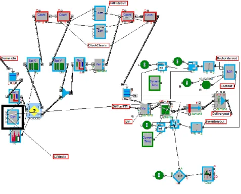
6.1 Extend ... 43
6.2 The Simulation Model ... 43
6.3 Simulation Approach ... 46
7 Results and Analysis ... 47
7.1 Expected Service Levels ... 47
Retailers ... 48
Upstream demand ... 50
Effect of increasing customer order sizes ... 52
Effect of fraction of upstream demand on CW fill-rate ... 54
7.2 Expected Inventory Levels ... 55
Central warehouse ... 56
Effect of fraction of upstream demand on CW inventory ... 58
7.3 Impact of Assumptions ... 59
The BM-model ... 59
Upstream demand in the empirical data ... 59
The use of a virtual retailer with lead-time zero ... 60
7.4 Sensitivity Analysis... 61
Local search for near-optimal S-levels ... 61
Local search for near-optimal reorder points ... 63
8 Conclusions ... 65
8.1 Achieving target fill-rates and reducing inventory ... 65
8.2 Potential of a critical level policy... 65
8.3 Uncertainty in the extracted data ... 66
8.4 Future Research... 66
References ... i
Appendices ... iv
Appendix A – table for determining normalized parameters ... iv
Appendix B - Tabulated Values of 𝒈 and 𝒌 Functions ... v
Appendix C – Table and Description of Results ... vi
1 INTRODUCTION
This chapter describes the background for the thesis. It also presents a problem definition, the purpose of the work, its delimitations, Syncron International and finally it discusses the target audiences and provides a chapter overview.
1.1 B
ACKGROUNDFor many companies a single warehouse is not sufficient to satisfy their network of customers. A common solution is to create a network of multiple central and regional warehouses, a so called multi-echelon inventory system. These systems have a flow of goods which enter at the central warehouse or warehouses that supply the retailers, which in turn deliver to the end customer.
When considering a multi-echelon system it is relatively simple to optimize each installation’s inventory levels separately, solely based on the demand they experience. However, from a cost perspective this approach is many times inefficient as the system as a whole might carry excess stock. There are large potential savings to be realized by instead coordinating the inventory control decisions for the system. That is, to optimize the overall cost and inventory levels in the entire network, while focusing on the service requirements of the end customers. This is the main purpose of multi-echelon modeling.
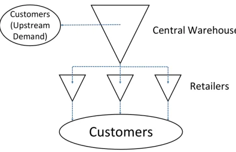
Because of geographical or business model reasons the central warehouse can be allowed to serve end customers, causing the phenomenon this thesis refer to as upstream demand. An example of a divergent multi-echelon system with upstream demand is depicted in Figure 1.
Customers
(Upstream
Demand)
Customers
Retailers
Central Warehouse
Figure 1- Divergent Multi-Echelon Inventory System with Upstream Demand One important aspect which makes modelling multi-echelon systems with upstream demand complex is that retailers and end customers usually have very different service requirements. This is problematic because when optimizing multi-echelon systems, stock is usually pushed from the central warehouse to the retailers. Consequently, the central warehouse gets a quite low measured service (Axsäter, et al., 2007), compared to the very high measured service at retailers.
Therefore, when both end customers and retailers are served from a central warehouse, either both demand classes will get a high service level and excess stock is carried in the system, or both will get a lower service and the end customer will not be satisfied.
One approach to meet the challenge of differentiating the service at the central warehouse to different demand classes, is to reserve stock for the high priority upstream demand. This can be accomplished by implementing a critical level policy. That is, when the stock at the warehouse is less than or equal to the critical level, only upstream demand is satisfied directly from stock while retailer orders are backordered (Axsäter, et al., 2007).
The global software provider, Syncron International, offer solutions that can help organizations manage their global supply chains. Syncron realize that a critical level policy has the potential to assist their customers in their
objective to reduce stock while still maintaining excellent service. As a result, Syncron is interested in evaluating the critical level policy by comparing its performance to real inventory data.
In previous cooperation between Syncron and Production Management at LTH, Berling and Marklund (2013, 2014) developed a multi-echelon model for a divergent system, the BM-model. In this model end customer demand only occur at the retailers. However, with slight modification, the model can also handle end customer demand at the central warehouse. In this thesis the BM-model will incorporate a critical level policy and its performance will be compared to inventory data, provided by one of Syncron’s customers.
1.2 P
ROBLEMD
ESCRIPTIONThis thesis will evaluate the BM-model presented by Berling & Marklund (2013; 2014) in a divergent multi-echelon setting with end customer demand at all locations. This model is chosen because of its flexibility in handling different demand distributions as well as its computational and conceptual simplicity. Parts of it has also been implemented in Syncron’s inventory management software.
The main challenge is that the BM-model has to be able to differentiate between the service requirements for end customers and retailers at the central warehouse. Focus is put on evaluating how well the BM-model performs, in terms of reaching target service levels (TSL) with as little expected inventory as possible.
This leads to the following questions that the thesis aim to answer: What impact does reserving stock have on the precision of
achieving TSLs?
What are the potential reductions in total inventory compared to the real inventory data, when reserving stock at the central warehouse for end customer demand?
How does the fraction of upstream demand affect the potential reductions in inventory?
1.3 P
URPOSEThe purpose of this thesis is to evaluate the performance of the BM-model in a one warehouse, multiple retailer system with upstream demand. This will be achieved by performing a comparison between empirical data, provided by one of Syncron’s customers, and analytical computations based on the BM-model.
The comparison will be performed with the help of simulation models, which are created to represent the real inventory system. The performance will be evaluated with respect to expected service levels and expected inventory levels.
1.4 S
YNCRONI
NTERNATIONALThe empirical data is provided by Syncron International which is a global “Software as a Service” (SaaS) provider that specializes in managing complex global supply chains. They have customers in over 100 countries and offices in a handful countries over the world. In Sweden they have offices in Stockholm, the global headquarters, and in Malmö.
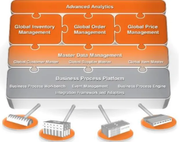
There are four main products in Syncron’s software; Inventory Management, Pricing Management, Order Management and Master Data Management. They also offer services in advanced analytics. Figure 2 presents a conceptual model showing how all of Syncron’s offers ties in to each other. This thesis is performed in connection to their Inventory Management Software, IM.
Figure 2 - Conceptual model of Syncron’s service offerings. Source: Syncron (2015)
The IM software offers companies the potential to reduce stock and increase end-customer stock availability by differentiating products, reallocating inventory and eliminating excess and obsolete stock. They offer both single- and multi-echelon modeling and tailor solutions to the customer.
1.5 D
ELIMITATIONSThis thesis will cover a divergent multi-echelon inventory system with one central warehouse and several retailers. Empirical data have been collected from one of Syncron’s customers, who wish to be known only as the case company. The data is restricted to items with customer demand at both retailer and central warehouse. All items are spare parts, or share characteristics with them. The results will be limited to measured service levels and expected inventory levels, no costs will be covered. The service
measure used in this thesis is the demand fill-rate1, also referred to as the
service level throughout the thesis.
1.6 T
ARGETA
UDIENCEThe target audience for this thesis are Syncron, people working for the case company as well as inventory management students and professionals with an interest in inventory control.
1.7 D
ISPOSITIONThe disposition in this thesis is based on a separated model for master theses by Blomkvist & Hallin (2014). It moves logically through the thesis based on a chronical setup, even if the thesis process in itself was iterative. The most important parts of this thesis, for all readers, are the adopted method in Section 2.1.2, the results in Chapter 7 and the conclusions in Chapter 8.
Chapter 1 – Introduction
This chapter describes the background for the thesis. It presents a problem definition, the purpose of the work, its delimitations and Syncron International. It also discusses the target audience.
Chapter 2 – Methodology
This chapter begins with a description of a general approach for operations research projects from the literature. This is followed by an adapted framework which is modified to align with the purpose of this thesis. The chapter ends with a description of some general scientific approaches and concepts as well as the positioning of the thesis in this context.
Chapter 3 – Theoretical Framework
This chapter covers the theory on which this thesis is based. First a literature review is presented which describes existing research conducted in the same field of study. This is followed by a description of the heuristic used in the main model for this thesis. Finally a section on different service level classifications will end this chapter.
Chapter 4 – Data Collection and Analysis of Input Data
This chapter describes the collection of data from the case company as well as the process of converting that data into useful information for this thesis. How the selection procedure of items to study were performed is also described.
Chapter 5 – Analytical Calculations
This chapter will present the procedure of using the BM-model in order to obtain reorder points. Furthermore the modifications to the BM-model are described. The chapter ends with a description of the recalculation of reorder points.
Chapter 6 – Simulation
This chapter explains the simulation modeling and analysis used in this work. Simulation is used to assess the performance of the analytical method used for obtaining reorder points for all the different stock points in the system.
Chapter 7 – Results and Analysis
In this chapter the results from studying the simulation will be presented. Focus is put on measured service levels and expected inventory levels. Then the results as well as assumptions will be discussed and analyzed in order to help the reader understand the results. Finally the results of the sensitivity analysis are presented.
Chapter 8 – Conclusions
This chapter will present a short summary of the key components of the analysis. Followed by a remark of what future research may be undertaken to further validate the results of this study.
2 METHODOLOGY
This chapter begins with a description of a general approach for operations research projects from the literature. This is followed by an adapted framework which is modified to align with the purpose of this thesis. The chapter ends with a description of some general scientific approaches and concepts as well as the positioning of the thesis in this context.
2.1 O
PERATIONSR
ESEARCHAs organizations grow, the complexity of its operations increases and new challenges and problems arise. One common problem is that when specialization and complexity in organization increases, it gets more difficult to allocate available resources to various activities in a way that benefits the organization as a whole (Hillier & Lieberman, 2001). As a result, individual units in an organization might grow into autonomous entities with their own goals and lose sight of the overall objective (Lieberman and Hiller, 2001).
Problems and challenges like these paved the way for the emergence of Operations Research (OR). OR uses mathematical modelling to provide near-optimal solutions for complex decision-making problems i.e. provide the best course of action (Hillier & Lieberman, 2001).
In the following sections, an overview of the generic Operations Research modeling approach described in Lieberman and Hillier (2001) will be presented, followed by the adapted framework which is more suited for the purpose of this thesis.
The Generic Operations Research Modeling Approach The purpose of this section is to present an overview of the major phases of an Operations Research study, as presented by Lieberman and Hillier (2001). Even though mathematical modelling plays a major role in OR, it often represents a relatively small part of the total effort required (Hillier & Lieberman, 2001), as the following section will demonstrate.
The generic modeling approach can be divided into six steps: 1. Define the problem of interest and gather relevant data.
Formulate a clear statement that describes the problem of interest. Gather relevant data to gain understanding of the problem and to provide input to the mathematical model. 2. Formulate a mathematical model to represent the problem.
Translate the studied problem into a form that is convenient for analysis. Mathematical modeling simplifies the problem with the help of assumptions and approximations, while still capturing the essential challenges and reveal cause-and-effect correlations. 3. Develop a computer-based procedure for deriving solutions
to the problem from the model.
Develop a procedure to be able to execute the mathematical model and determine near-optimal solutions. A well formulated and tested model should provide a good approximation of the best course of action.
4. Test the model and refine it as needed.
Model verification to find and remove errors and model validation to establish that the model captures the ideas and concepts of the studied problem.
5. Prepare for the ongoing application of the model as prescribed by management.
Install a system for applying the model as prescribed by management. The system includes the model, the solution procedure and operating procedures for implementation. 6. Implement.
Implementation of the system, including the mathematical model.
The Adapted Operations Research Modeling Approach The modelling approach described in the previous section has to be adjusted to fit the purpose of this thesis. The most notable difference is that the fifth and sixth steps will be disregarded as implementation is outside the scope of this thesis. Furthermore, time will not be spent on developing a new analytical model. Instead we adapt an existing model that has been proposed for handling upstream demand, but which has never been tested in this respect. More details regarding the existing model can be found in Section 3.2.
The adapted modeling approach contains the following steps: 1. Define the problem of interest and gather relevant data 2. Perform data analysis and select items to study
3. Modify the existing model and derive solutions
4. Evaluate the model by comparison through simulations 5. Analyze the results and refine if needed
Each of these steps are further explained below.
1. Define the problem and gather relevant data
The problem definition originated from discussions with representatives from Syncron and Production Management at LTH. Syncron were interested in evaluation of an inventory policy that can be applied to an inventory system with upstream demand. In previous cooperation, Berling and Marklund (2013, 2014) developed a multi-echelon model, the BM-model, for a divergent system where end customer demand only occur at the retailers.
However, with slight modification, the model can also handle end customer demand at the central warehouse. This aspect of the model had so far not been evaluated. Consequently the purpose of the master thesis was created to evaluate the performance of this model when allowing customer demand at the central warehouse as well. The evaluation will be carried out through simulations, by comparing the BM-model with N+1 uncoordinated single-echelon models. Real data from a case company will be used as input and the performance will be assessed based on the two models’ ability to reach target service levels and the total expected inventory.
To gather relevant data, a literature study was performed which can be found in Section 3.1. The purpose of this study was to acquire an understanding of the academic research that is available on the topic of upstream demand, in both single- and multi-echelon settings. Later, this study was extended to include research on stock rationing and multiple demand classes as these areas also cover inventory policies which involve demand streams with different service requirements or priority.
The data from practice was provided by the case company. Data analysis and manipulation will be covered in the next section.
2. Perform data analysis and select items to study
The purpose of using data from practice as input is twofold, using data from the case company facilitates the comparison as parameters such as order quantities, target service levels and lead-times are readily available. Furthermore, fictional data would be difficult to construct in a way that captures the sometimes elusive nature of demand patterns. Hence, by using fictional data some of the challenges of inventory control in practice may be lost in the process. More details regarding the empirical data can be found in Section 4.1.
The items for the study are selected based on a list of criteria that ensures that appropriate items are used. The sample size is set to be large enough to sufficiently capture a wide range of item characteristics but not too large as the study is rather time consuming. About 100 items is be considered enough for this purpose. The execution of this selection is described in Section 4.2.
For each of the selected items the mean and standard deviations of the demand per day were determined together with the distributions of the customer order sizes. These parameters can be derived from the extracted demand history, provided by the case company. This data analysis is further explained in Section 4.3.
3. Modify the existing model and derive solutions
The BM-model is originally constructed to model a pure multi-echelon system where customer demand only takes place at the retailers. However, it is also possible to let the model handle upstream demand by setting the transportation time to one of the retailers to zero. This retailer will be referred to as the virtual retailer and its inventory is reserved to only satisfy the upstream demand, see Figure 3. Furthermore, the virtual retailer replenishes its stock from the central warehouse using a continuous review (S-1, S) policy. Conceptually the central warehouse and the virtual retailer are modeled as separate stock points that are linked by the lead-time which
Customers (Upstream demand)
Customers
Retailers
Central Warehouse
with virtual retailer
(S-1, S)
(R
0, Q
0)
(R
1, Q
1)
(R
i, Q
i)
(R
N, Q
N)
1
. . . .
i. . . .
NƖ = 0
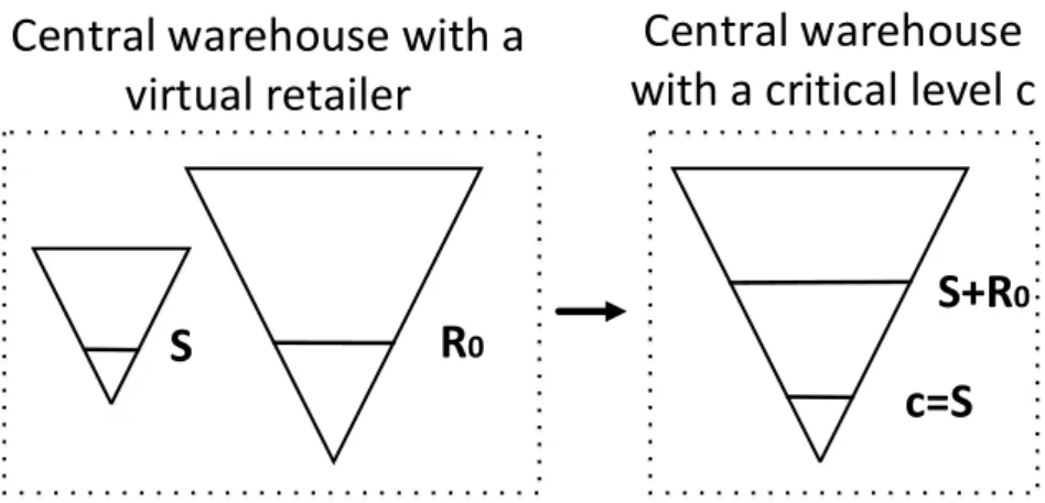
Figure 3- Divergent Multi-Echelon System with Upstream Demand and a Virtual Retailer The approach to model with a virtual retailer can be viewed as an approximation of a so called critical level policy. This policy defines a nonnegative critical level c for stock on hand at the central warehouse. If the stock on hand is less than or equal to c, only customer demand is satisfied while retailer orders are backordered (Axsäter, et al., 2007). As there are two stock locations in the approximation, the central warehouse reorder point of a critical level policy can be approximated as
S+R0. Furthermore, the critical level c can be approximated by S, as
S
R
0S+R
0c=S
Central warehouse with a
virtual retailer
Central warehouse
with a critical level c
Figure 4 - Illustration of the Relationship Between a Central Warehouse with a Virtual Retailer and a Central Warehouse with a Critical Level c.
Based on the input parameters derived from the empirical data, the BM-model is used to determine near-optimal reorder points for all stock locations, including the S-level at the virtual retailer. More details regarding deriving solutions from the BM-model can be found in Section 5.1.2.
4. Evaluate the model performance using simulation
In order to evaluate the performance of the model, simulations are used where simulation models are created for each individual item to emulate the real inventory system. The comparison consists of simulating each item two times, where the reorder points are the only input parameters that are changed between simulations. The studied reorder points are the ones determined with the BM-model as well as reorder points from N+1 uncoordinated single-echelon models. The results from the simulations include expected service levels and expected inventory levels for each stock location including the virtual retailer.
5. Analyze the results and refine as needed
As this study consists of a number of steps where data is manually inserted and all these steps are repeated for all items in the study, there is a risk of making a mistake somewhere. To reduce this risk a check list was used which systematically explained the procedure step by step. In addition to the check list, the results in each step were analyzed to detect any
unreasonable values and to get a chance to correct any errors that could occur.
2.2 S
CIENTIFIC APPROACHThere are a vast array of scientific approaches that are relevant when conducting an operations research study. This include, but is not limited to, what the study is trying to accomplish, what the process looks like and what data analysis method that will be used.
Explorative, Descriptive, Explanatory and Normative
The type of study that is used depend on the existing body of knowledge in the particular area (Björklund & Paulsson, 2014).
An explorative or investigatory study is used when there are little knowledge in the area and the purpose is to attain fundamental knowledge. A descriptive study builds on the existing knowledge by describing the existing correlations without explaining. Explanatory studies strive for deeper knowledge in an area and seek to both describe and explain. Finally, normative studies are used when there are already knowledge and understanding in the area and the objective is to provide further guidance and prescribe what to do (Björklund & Paulsson, 2014).
Based on these classifications this thesis will contain elements of an explanatory study, as the purpose is to gain deeper knowledge in a specific area which has already been described in previous research.
Deductive and Inductive
Research approaches may also be classified as deductive or inductive2. The
deductive process, also known as theory testing process, starts with a known theory and aims to test if it applies in a certain context (Spens & Kovács, 2006). The inductive process does the opposite and starts with an observed phenomenon and seek to generalize it into a new theory (Spens & Kovács, 2006).
This thesis will use both the deductive and inductive approach. It is deductive due to the fact that the BM-model can be classified as known and ratified theory and the objective is to test its performance in another
2 Some argue for a third approach, abductive, as a mix of the deductive and the
context. However, the study is inductive when it comes to understanding and explaining the observed results.
Quantitative and Qualitative
Research can also be classified as qualitative or quantitative. According to (Spens & Kovács, 2006) this classification should be decided based on which data analysis technique is used and not the means of gathering data. Qualitative research is all research that does not use statistical measures or try to quantify the problem (Golafshani, 2003). Quantitative research aim to generalize findings and to find a casual determination (Golafshani, 2003). Within logistics, quantitative research is most often conducted with numerical data analysis (Spens & Kovács, 2006).
This study will mainly use quantitative analysis and conduct numerical data analysis. There will be qualitative aspects to the final results but those are not the main focus but rather a result of data anomalies that need further investigation.
2.3 Q
UALITYD
IMENSIONSThere are several different dimensions when assessing quality. Näslund (2002) classifies the quantitative research as part of the Positivist paradigm. To this paradigm he pairs four criteria for good research; Internal validity, external validity, reliability and objectivity. This section will explain these criteria with respect to the thesis and its operations research approach.
Validity
Validity is a way to assess if the observations in a study in a meaningful way capture the ideas and concepts it studies (Adcock & Collier, 2001). Potential validity issues can be caused by delimitations or assumptions in the model. Näslund (2002) divides validity into two parts, external and internal. Where internal is how well the model represents the reality and external concerns how transferable the results are to other similar situations as those studied.
As this study does not include the development of a new model but instead utilize the existing BM-model, validity is not an issue. The BM-model has been thoroughly tested and used in previous academic research and theses, its internal validity is well-grounded. Furthermore, regarding its external validity, it is constructed with few restrictions but many options which makes it valid for many divergent multi-echelon systems.
Reliability
Reliability concerns how replicable an observation or result is (Golafshani, 2003). This is important because if the results cannot be established as reliable then they are of little use. A reliable result will be the same, within specified limits, when the test is repeated in order for the results to be trusted. It is important to remember that reliability does not say anything about the correctness of the result just the ability of the method or tool used to consistently produce the same result.
The main aspect that affects the reliability of the results in this study is not the model itself but the human factor. This is due to the fact that data is manually inserted in several steps. To reduce the risk of creating errors a check list is created in combination with careful analysis of the results in each step in order to expose anomalies.
Furthermore, the simulation model, that is used to evaluate the performance in this study, has been thoroughly tested in previous research. The minor changes that are made are tested to make sure that the model operates as it is intended.
Objectivity
This quality dimension concerns how free the results are from bias (Näslund, 2002). By clarifying and motivating the different choices made in the study the reader is given the possibility to reflect on the course of action as well as the results of the study (Björklund & Paulsson, 2014). When using synopses of other author’s papers, objectivity problems can arise (Björklund & Paulsson, 2014). It is a matter of recounting the content in an unbiased manner by, first and foremost, reciting statements without any factual errors. Secondly, there should be no distorted selection of facts or arguments, with the purpose to support your own point of view. Finally, one should avoid the using a negative vocabulary which can give the impression that the original author has an erroneous perception.
The main purpose of the thesis is not to promote nor try to prove the efficiency of a method. The purpose is to observe the results and try to understand and explain why the results are as they are, without an agenda. Furthermore, the papers included in the literature review (see Section 3.1) are not selected to prove a certain point. Instead they are selected to illustrate what academic research that has been conducted in the area of upstream demand, multiple demand classes and stock rationing.
3 THEORETICAL FRAMEWORK
This chapter covers the theory on which this thesis is based. First a literature review is presented which describes other academic research conducted in the same field of study. This is followed by a description of the heuristic used in the main model for this thesis. Finally a section on different service level classifications will end this chapter.
3.1 L
ITERATURER
EVIEWThe purpose of the literature review is to position this thesis in relation to the existing literature. Following are a number of inventory models that are developed for handling multiple demand classes with different service requirements. This typically means the use of critical level policies or general stock rationing policies. As mentioned in Section 2.1.2, a critical level policy essentially means that some inventory is reserved for a demand class which have higher service requirements. The first section covers models for single-echelon systems, followed by a section for multi-echelon systems.
For a single-echelon inventory model the objective is to optimize the inventory decisions at a single stock location, independent of the other stock locations. Consequently, when using single-echelon optimization in a system with several stock locations, the inventory at each stock location is sub-optimized.
In multi-echelon optimization the objective is to optimize the inventory decisions for the entire system according to certain objectives. Usually these objectives involve minimizing the overall expected costs. When modelling with service constraints this means that only stock locations which face customer demand need to reach a certain target service. Furthermore, the lead-time between stock locations depends on the risk of stock-out at the supplying location.
Single-echelon models with critical level policy
Dekker et al. (2002) use an (S-1, S) policy with lost sales and can show that a critical level policy outperforms the first-come, first-serve policy (FCFS). The total cost savings when using service constraints have an average of 33.3% and show the largest savings when the majority of demand is in the lower service level class (Dekker, et al., 2002).
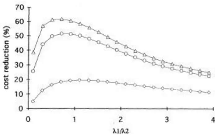
Ha (1997) investigated the use of a critical level in combination with an (s, S) policy, several demand classes and lost sales. This means that the objective is to minimize the total expected holding and lost sales costs. He finds that the potential cost savings are strongly related to the ratio between
the high priority demand rate (λ1) and the low priority demand rate (λ2),
Figure 5. The largest cost reduction occur when the high priority demand is equal to or slightly smaller than the low priority demand (Ha, 1997). Furthermore Ha discusses that when arrivals of customers of one demand class is rare, the cost reductions are very small. This is because the system in those cases is close to a system with a single demand class.
Figure 5 - Cost Reduction when Using versus Demand Ratio for Three Examples with Different Lost Sales Cost Structures (Ha, 1997)
Melchiors et al. (2000) investigates a combination of a critical level and a (R, Q) policy with lost sales and two demand classes. They find that the cost reductions vary depending on whether the critical level is larger or smaller than the reorder point. When the critical level is larger, cost reduction of up to 50% were recorded. When it was instead smaller than the reorder point, the maximum cost reduction were only 10% and that was in a situation where the cost of lost sales were extremely high (Melchiors, et al., 2000).
They also found that the greatest cost reductions occurred when the high priority demand were between 10 to 25 percent of total demand. Finally the authors also conclude that it might be cost efficient to let the policy be lead-time dependent. That is, low priority demand can be satisfied even though the inventory is below the critical level if there is a certain time left before a replenishment order from the supplier arrives.
Wang and Tang (2014) study a system with a mix of demand classes with backorders as well as lost sales. Furthermore, it consists of multiple periods where the inventory level is replenished at the start of each period with a lead-time of zero. The critical levels are dynamic and changes over time. They conclude that the average cost reductions are slightly above 10 percent and they also conclude that rationing policies are close to useless when one of the demand classes is dominant (Wang & Tang, 2014). Nahmias and Demmy (1981) analyze the effects of using a critical level in combination with a (R, Q) policy with both continuous and periodic review. Given a certain combination of reorder points and order quantities, they construct tables with resulting fill-rates for both with and without stock rationing. They conclude that stock rationing can achieve higher fill-rates than without stock rationing, given a certain reorder point (Nahmias & Demmy, 1981).
Moon and Kang (1981) use an (R, Q) policy with compound Poisson and a critical level to be able to differentiate between demand classes. They also add several critical levels and study how the expected number of backorders for the different demand classes changes (Moon & Kang, 1998). They conclude that by using stock rationing it is possible to efficiently satisfy different demand classes.
A conclusion that many of these papers have in common is that a critical level policy is most valuable when a minority (≈10-40%) of the total demand is of higher priority. However, if one demand class is dominant (>90%), a critical level policy yields no better result than a regular FCFS policy.
Multi-echelon models with critical level policies
In a Multi-Echelon setting there are very few studies made on continuous review systems with stock rationing. One problem seems to be that there are no known exact mathematical solutions, instead numerical studies using simulation is required. (Axsäter, et al., 2007).
Axsäter et al. (2004) use a (S-1, S) policy with lost sales and multiple demand classes. They also find that a critical level policy leads to cost savings, in this case often around 5%. They also state that in more extreme cases, substantially larger cost reductions are possible (Axsäter, et al., 2004).
Numerical results shows that the critical level policy performs better than both standard FCFS, as expected, and the so called separate stock point policy (Axsäter, et al., 2007). The separate stock point policy uses a virtual retailer which carry stock and only serve the high priority demand. This is the same approach that is used in this thesis and is described in Section 2.1.2.
The advantage of a critical level policy over separate stock policies is not clearly stated in the article but could be due to the fact that the results for the critical level policy are obtained by simulation while the results for the separate stock point policies are analytically calculated. The separate stock policy has the advantage that it can be evaluated and optimized without special treatment for direct demand (Axsäter, et al., 2007). Using simulation to determine policy parameters is not feasible for large real world systems.
3.2 T
HEBM-M
ODELThis section will describe the models presented in Berling and Marklund (2013; 2014). The models are similar with the important exception that the retailer demand is modelled by a normal distribution in Berling and Marklund (2014), and a compound Poisson distribution in Berling and Marklund (2013). Therefore the models will be treated as one, here referred to as the BM-model, with two options on retailer demand. The authors also conclude that it is possible to combine these models (Berling & Marklund, 2014).
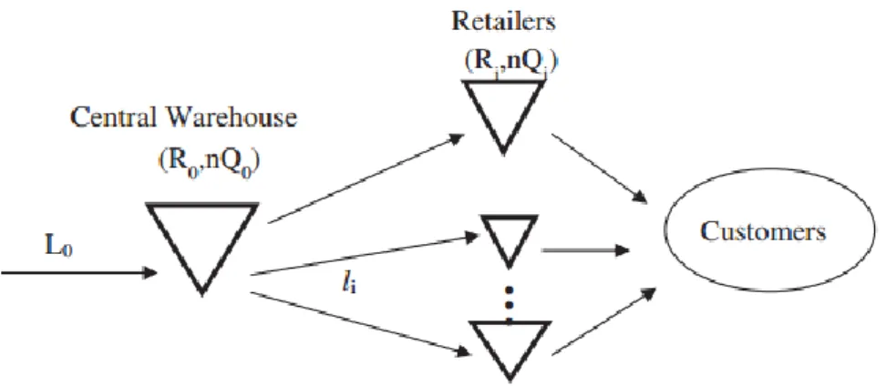
Figure 6 depicts the considered one-warehouse, N-retailer system. All
stock-points use continuous review (Ri, nQi) policies to replenish their
inventory. This means that when the inventory position3 reaches or falls
below R, an order is triggered to get the inventory position back above R.
Orders are placed as integer multiples, n, of the fixed order quantity Qi at
each installation. The central warehouse replenishes from a supplier that is assumed to have an infinite amount of stock. (Berling & Marklund, 2014)
Figure 6 – Multi-Echelon Inventory System with a Central Warehouse and N Non-Identical Retailers. Source: (Berling & Marklund, 2014)
The BM-model assumes that complete backordering and partial deliveries are used. Furthermore, FCFS policies are employed throughout the system.
The lead-time, L0, from a supplier to the central warehouse as well as the
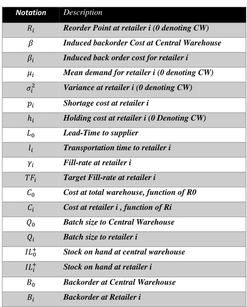
transportation times to the retailers from the central warehouse are assumed to be constant. However, lead-times to retailers are stochastic due to the possibility of stock outs at the central warehouse. The notation used in this chapter can be found in Table 1.
Table 1- Notations used in the BM-Model
Notation Description
𝑅𝑖 Reorder Point at retailer i (0 denoting CW)
𝛽 Induced backorder Cost at Central Warehouse
𝛽𝑖 Induced back order cost for retailer i
𝜇𝑖 Mean demand for retailer i (0 denoting CW)
𝜎𝑖2 Variance at retailer i (0 denoting CW)
𝑝𝑖 Shortage cost at retailer i
ℎ𝑖 Holding cost at retailer i (0 Denoting CW)
𝐿0 Lead-Time to supplier
𝑙𝑖 Transportation time to retailer i
𝛾𝑖 Fill-rate at retailer i
𝑇𝐹𝑖 Target Fill-rate at retailer i
𝐶0 Cost at total warehouse, function of R0
𝐶𝑖 Cost at retailer i , function of Ri
𝑄0 Batch size to Central Warehouse
𝑄𝑖 Batch size to retailer i
𝐼𝐿0+ Stock on hand at central warehouse
𝐼𝐿𝑖+ Stock on hand at retailer i
𝐵0 Backorder at Central Warehouse
𝐵𝑖 Backorder at Retailer i
The BM-model incorporates two options for service requirements (Berling & Marklund, 2013). The first one is the service level model, where the objective is to minimize the expected holding costs while meeting the specified target service levels. The second option is the backorder cost model, where the objective is to minimize the expected backorder and holding costs, without adding any service level constraints. This master
thesis only uses the service level model, therefore the backorder cost model will not be explained any further.
The BM-model makes use of an induced backorder cost, β, which should capture the costs at the retailers due to the delivery delays at the central warehouse. Using this induced backorder costs makes it possible to decompose the multi-echelon system into N coordinated single-echelon systems (Berling & Marklund, 2006) which are possible to solve using installation stock policies.
This approach was first presented in Andersson et al. (1998) where βi is
defined as the expected marginal cost with respect to retailer i’s lead-time. Later this method was used in Berling and Marklund (2006), to estimate closed form estimates of a near-optimal β-value, which are conceptually and computationally simple to use.
How to Use the Heuristic
The BM-Model can be divided in five steps. These steps are performed in sequence once, which explains why the model is computationally possible to use for large problems. The steps are (Berling & Marklund, 2014):
1. Determination of near optimal induced backorder cost 2. Determination of lead-time demand at the central warehouse 3. Determination of reorder point at central warehouse
4. Determination of lead-time demand at each retailer 5. Determination of reorder points at each retailer 1. Determination of near optimal induced backorder cost
The induced backorder cost, β, is an approximation of the cost caused by the central warehouse when it fails to deliver as ordered. This includes both the cost for safety stock and the shortage cost at the retailers (Berling & Marklund, 2014).
To estimate the induced backorder cost associated with retailer i, the approach in Berling and Marklund (2006) is used. This approach first
normalizes the system parameters with respect to the tranportation time (li),
the mean demand (µi) and the holding cost (hi). The table which shows
how to move between the original and normalized parameters can be found in Appendix A – table for determining normalized parameters.
One of the system parameters is the shortage cost (pi), which is not directly
available in a model with service level constraint. However, it can be estimated with the help of the corresponding target fill-rate by using the optimality condition (Axsäter, 2006) which is described as a relation between fill-rate, holding- and shortage costs in (1). The optimality condition is exact for normally distributed demand but has shown to work as a good approximation for other distributions as well in the context of the BM-model (Berling & Marklund, 2014).
𝑇𝐹𝑖 =
𝑝𝑖
ℎ𝑖+ 𝑝𝑖
(1)
Each retailer’s induced backorder cost, βi, is calculated according to (2)
which uses the closed form estimate from Berling and Marklund (2006).
β𝑖 = ℎ𝑖∗ 𝑔(𝑄𝑖,𝑛, 𝑝𝑖,𝑛) ∗ 𝜎𝑖,𝑛
𝑘(𝑄𝑖,𝑛,𝑝𝑖,𝑛)
(2)
An alternative to the closed form expressions is to use tabulated values of
𝑔(𝑄𝑖,𝑛, 𝑝𝑖,𝑛) and 𝑘(𝑄𝑖,𝑛, 𝑝𝑖,𝑛) , which can be found in Appendix A.
Between parameter values in the tables, linear interpolation may be used,
and outside of the table range the closed form expressions for 𝑔(𝑄𝑖,𝑛, 𝑝𝑖,𝑛)
and 𝜎𝑖,𝑛𝑘(𝑄𝑖,𝑛,𝑝𝑖,𝑛) need to be used.
The induced backorder cost for the central warehouse is then estimated as
a demand weighted average of the different β𝑖′𝑠. The weighting method
for the induced backorder cost at the central warehouse can be found in (3) and its performance is established in (Berling & Marklund, 2006). The main reason for selecting this weighting formula is that it has shown near-optimal results and not performing significantly worse than other plausible but more complex weighting schemes (Berling & Marklund, 2014). It is therefore the best option based on its simplicity.
β =∑ 𝜇𝑖β𝑖
𝑁 𝑖=1
∑𝑁𝑖=1𝜇𝑖
2. Determination of lead-time demand at the central warehouse The BM-model approximates the true lead-time demand distribution by using three standard distributions based on the variance-to-mean ratios (Berling & Marklund, 2014). The three standard distributions are;
Negative Binomial, when 𝜎02
𝜇0 ≥ 1
Discrete normal approximation, if 𝜎02
𝜇0< 1 𝑎𝑛𝑑
𝜎0
𝜇0< 0.25
Discrete gamma approximation for all other cases.
This approximation scheme is used to improve the computational performance of the model which would have decreased considerably if the true lead-time distribution is used. Berling and Marklund (2014) show that this approximation typically render the same reorder points as the true distribution. Consequently, the lead-time demand at the central warehouse is approximated by fitting distributions to the correct mean (4) and variance (5). µ𝑜 = µ01+ µ02+ ⋯ + µ0𝑁 𝑤ℎ𝑒𝑟𝑒 µ0𝑖 = µ𝑖𝐿𝑜 𝑄 (4) 𝜎02= (𝜎01)2+ (𝜎𝑜2)2+ ⋯ + (𝜎𝑜𝑁)2 (5) 𝑤ℎ𝑒𝑟𝑒 (𝜎𝑜𝑖) 2 = ∑(𝜇0𝑖 − 𝑛𝑞𝑖 ∞ 𝑛=0 )2𝑔0𝑖(𝑛𝑞𝑖)
The variance of the lead-time demand at the central warehouse depends on
the number of retailer orders that are triggered during L0. Defining,
𝐷0𝑖(𝐿
0), as the sub-batch demand from retailer i during L0 time units and
its probability mass function 𝑔0𝑖(𝑢) according to (6), we have:
𝑔0𝑖(𝑢) = 𝑃(𝐷0𝑖(𝐿0) = 𝑢) = = { 𝛿𝑖(0) 𝑖𝑓 𝑢 = 0 𝛿𝑖(𝑛) − 𝛿𝑖(𝑛 − 1) 𝑖𝑓 𝑢 = 𝑛𝑞𝑖, 𝑛 = 1,2, . . . 0 𝑜𝑡ℎ𝑒𝑟𝑤𝑖𝑠𝑒 (6)
3. Determination of the reorder point at central warehouse, R0
When the induced backorder cost and the distribution of the lead-time
demand is known, the reorder point at the central warehouse (R0) can be
determined by minimizing the expected holding and induced backorder costs. (Berling & Marklund, 2014). This cost function can be found in (7).
𝐶0= ℎ0𝐸[𝐼𝐿+0(𝑅0)] + 𝛽𝐸[𝐵0(𝑅0)] (7)
Since the cost function is convex in R0 the optimal reorder point for the
central warehouse can be found by a simple search while applying the condition in (8). (Berling & Marklund, 2014)
𝑅0= max {𝑅0: 𝐶0(𝑅0) − 𝐶0(𝑅0− 1) ≤ 0} (8)
4. Determination of lead-time demand at each retailer
The replenishment lead-time to retailer i, and the associated lead-time
demand, are functions of R0. In this step Berling and Marklund (2014) use
two different methods for calculating the variability of the lead-time. Both methods use an approximated mean for the lead-time (9) by applying Little’s law to find the expected warehouse delay (Berling & Marklund, 2014). 𝐿̅𝑖(𝑅0∗) = 𝜇𝛿(𝑅0∗) + 𝑙𝑖= 𝐿0 𝜇0𝑄𝐸[𝐵0(𝑅0 ∗)] + 𝑙 𝑖 (9)
When determining the standard deviation of the lead-time, the methods differ. The first method uses the METRIC approximation (Sherbrooke, 1968) which sets the lead-time variance to zero, basically disregarding it. The second method estimates the lead-time variability by adapting the method in Axsäter (2003). This method will not be used in this thesis as it is more computationally demanding and do not give better results (Berling & Marklund, 2014). Using the first approach, the mean and standard deviation of the retailer lead-time demand are then defined according to (10) and (11) respectively.
𝜇𝐷𝑖(𝐿𝑖)= 𝜇𝑖𝐿̅𝑖 (10)
𝜎𝐷𝑖(𝐿𝑖)= √𝜎𝑖
2𝐿̅
5. Determination of reorder points at each retailer
After the lead-time demand for each retailer is determined, the multi-echelon system is decomposed into N coordinated single-multi-echelon systems that can be optimized using single-echelon methods. The objective is to find the smallest reorder point that still satisfies the target service level. The optimal reorder point is easily found by performing a search until (12)
is satisfied, starting from Ri = −Qi and increasing Ri with integer steps.
𝑅𝑖= min{𝑅𝑖: 𝛾𝑖 ≥ 𝑇𝐹𝑖} 𝑓𝑜𝑟 𝑖 = 1,2, … , 𝑁 (12)
The service level requirements are calculated according to (13), fill-rate calculation under the assumption of normal demand, and (14), fill-rate calculations for compound Poisson demand (Berling & Marklund, 2013, 2014). 𝛾𝑖 = 1 − 𝑃(𝐼𝐿𝑖 ≤ 0) = = 1 − (𝜎𝐷𝑖(𝐿𝑖) 𝑄𝑖 [𝐺 ( 𝑅𝑖−𝜇𝐷𝑖(𝐿𝑖) 𝜎𝐷𝑖(𝐿𝑖) ) − 𝐺 ( 𝑅𝑖+𝑄𝑖−𝜇𝐷𝑖(𝐿𝑖) 𝜎𝐷𝑖(𝐿𝑖) )]) (13) 𝛾𝑖 = ∑∞𝑑=1∑∞𝑗=1min(𝑗,𝑑)𝑓𝑖(𝑑)𝑃(𝐼𝐿𝑖=𝑗|𝑅𝑖) ∑∞𝑑=1𝑑𝑓𝑖(𝑑) (14)
The underlying assumption in the normal distribution is that all customer orders arrive continuously which create problems in this approach. If the actual demand consists of customers with different order quantities it means that the inventory position falls below the reorder point before a replenishment order is triggered. The normal demand model on the other hand assumes that a replenishment order is triggered at the exact moment when the inventory level hits the reorder point. (Berling & Marklund, 2014)
Berling and Marklund (2014) uses two different undershoot adjustment methods to compensate for this property of the normal distribution. One based on realized reorder points and the other based on the mean and variance of the undershoot.
The method based on realized reorder points uses the assumption that the
inventory position is uniformly distributed on [Ri+1, Ri+Qi], which is a
probability of negative demand is small (Berling & Marklund, 2014). With the probability of an undershoot of size u, as presented in (15), it is possible to calculate the expected fill-rate for the following realized reorder point, as can be seen in (16). 𝑈𝑖(𝑢) = 1 𝑄𝑖∑ 𝑂𝑖(𝑘) 𝑢+𝑄𝑖 𝑘=𝑢+1 (15) 𝛾𝑖 = ∑𝑢𝑢=0̂ 𝑆𝐸𝑅𝑉1(𝑅𝑖− 𝑢)𝑈𝑖(𝑢) (16)
3.3 S
ERVICEL
EVELSThere are many ways to measure service levels. However, there are three main categories that covers most of the service level measurements;
Probability of no stock out during an order cycle, Fill-rate and Ready Rate4.
In this thesis Fill-rate will be used as the service level measurement and it will be defined as:
Fraction of demand that can be satisfied immediately from stock on hand – (Axsäter, 2006)
The reason fill-rate is used is that, except that it is easy to evaluate both theoretically and in practice, it only decreases when customers demand an item that is not in stock. Ready rate on the other hand decreases during stock outs, whether or not there are any current customer demand.
Probability of no stock out during an order cycle, SERV1, is easy to
conceptually understand and use in practice. However, SERV1 has one
great disadvantage, it does not take the order size into account. This means that when the order quantity is large this measurement will underestimate the service experienced by the customer. Consequently when the replenishment order quantity is small the experienced service (e.g. fill-rate)
can be low even if SERV1 is high. (Axsäter, 2006)
4 Also known as SERV
4 DATA
COLLECTION AND
ANALYSIS OF
INPUT DATA
This chapter describes the collection and analysis of the data from the case company as well as the process of converting that data into useful information for this thesis. How the selection procedure for items to study is also described.
4.1 D
ATAR
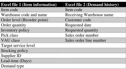
ECEIVEDIn order to use the BM-model as well as compare the results to the empirical data several parameters are needed. This material was provided by the case company and extracted from Syncron´s system. The data material was received as two excel files and contained item information as well as demand history for the studied inventory system. The parameters in the data material can be seen in Table 2. In response to a request from the case company, only the results from using this information will be presented in this thesis, and not the data itself.
Table 2 - Case Company Data Extracted from IM
Excel file 1 (Item information) Excel file 2 (Demand history)
Item code Item code
Warehouse code and name Receiving Warehouse name
Order level (Reorder point) Customer code
Order quantity Requested date
Inventory policy Requested quantity
Pick class Sales order number
VAU class Sales order line number
Target service level Stocking policy Supplier ID Lead-time (Days) Demand type
Some of the parameters in Table 2 are only of practical use for keeping track of and sorting items, suppliers, customers and warehouses. The following parameters are needed for the numerical study:
Demand history
This will be used to determine a statistical distribution to represent the item’s demand pattern. The demand covers three years back from October 2015 and an assumption was made that all items were introduced before the start of this time period. The most important parameters are the requested date and requested quantity which are needed to calculate the mean and standard deviation of the demand per day, for all selected items. In total the demand history consisted of over 300 000 transactions.
Lead-times
In order to determine the safety stock levels properly, the replenishment times are essential. The replenishment times from the case company are the agreed times between order and delivery. The historic data does not account for stock out delays at the warehouse. This is however calculated in the BM-model.
Target service level
As the real inventory system is optimized using single-echelon methods with service constraints, all stock locations including the central warehouse has a target service level. However, the target service level for the central warehouse is not used in the BM-model as it uses multi-echelon optimization.
Order quantities
This thesis will use the fixed order quantities from the real data. This is because even though it is possible to calculate the Economic Order Quantity, often restricted by other factors. Optimizing the order quantities also requires information regarding the order set up costs which are not available from the case company.
Order level (Reorder point)
The reorder points in Syncron´s system are calculated as uncoordinated single-echelon installations with normal, Poisson or negative binomial distribution to approximate the demand. The reorder points are important because they are needed in the situation for comparison with the analytical model’s reorder points to. As explained in Section 5.2 some of the extracted reorder points were later recalculated in order to get a more fair comparison of the performances of the models.
One parameter which would intuitively seem important but have been disregarded in this thesis is the holding cost rate at central warehouse and retailers. After discussion with Syncron it has been concluded that the holding cost rates are the same at all stock-points since this is generally how most of the customers have their setup, including the case company. As a result, minimizing the total expected inventory is equivalent to minimizing the expected holding costs.
4.2 I
TEMS
ELECTIONThere are several ways of selecting the data for a quantitative study. The broadest distinction is between random and non-random samples.
Non-random samples include comfortability selection5 and yes-sayer selection6
(Blomkvist & Hallin, 2014). The random sampling methods include complete random selection, systematic random selection, cluster selection and proportional stratified selection (Blomkvist & Hallin, 2014). If the aim for the study is to be able to extrapolate the results to a larger group than the sample, the random selections are preferable. This is because of the fact that non-random selection methods can end up with a large portion of bias. Initially the plan was to make the selection of items in two steps, where the first step included setting up a number of criteria in order to remove the items that did not fit the scope of the thesis. The second step would then be to perform a stratified selection to select a range of items that represented the overall characteristics of the entire product assortment. Even though the data consisted of more than 4000 stocked items, only a few hundred items fulfilled the list of criteria that was set up. Therefore the stratified selection were deemed unnecessary and the items were instead selected solely based on the following list of criteria.
1. Items stocked in central warehouse 2. Items stocked at no less than two retailers
3. Items with at least 10 transactions per stock location
With the help of these criteria 92 items were chosen to represent the case company’s article range in this study.
5 Using the data which is easiest to obtain 6 Use those that want to be a part of the study
4.3 D
ETERMININGI
NPUTP
ARAMETERSIn order to be able to determine optimal reorder points in the BM-model, several input parameters and the order size distribution are required. These are as follows:
Mean demand per day
Standard deviation of demand per day Customer order size distribution Lead-time
Order quantity Target service level Holding cost
All parameters are needed for each item and stock location, including the virtual retailer facing the upstream demand at the central warehouse. Lead-time, order quantity and target service level were provided by the case company, the holding cost rate is assumed to be the same for all stock locations and is therefore, without loss of quality, set to one. Consequently, the first three input data on the list need to be calculated.
Distribution of demand at retailers
The mean demand is simply an average of the demand experienced at each stock location per day. The variance of the demand per day is estimated using (17). 𝑥̅ denotes the mean demand of n observations. Subsequently, the standard deviation of the demand per day is calculated as the square root of the variance.
𝑉𝑎𝑟 =∑𝑛𝑖=1(𝑥𝑖−𝑥̅)2
𝑛−1 (17)
The customer order size distribution i.e. the probability of customers ordering a certain number of units, are estimated from the data using relative frequencies. This mean that the number of orders of a certain unit size at each retailer is divided by the total number of orders at that retailer.
Mean and standard deviation for upstream demand
From the data received it was not possible to distinguish the upstream demand from retailer orders at the central warehouse. In order to estimate the upstream demand the following approach was therefore used.
The approach consisted of comparing the mean and standard deviation of the demand experienced at the central warehouse from the empirical data,
with the aggregated demand from the retailers as calculated in the
BM-model (see Section 0 for calculations of 𝜇0𝑖 and (𝜎0𝑖)2 for retailer i). If the
aggregated demand from the retailers is subtracted from the total demand
at the central warehouse, the remainder will equal the mean (𝜇𝑈𝐷) and
standard deviation (𝜎𝑈𝐷) of the upstream demand, as presented in (18) and
(19).
𝜇𝑈𝐷 = 𝜇0− ∑𝑛𝑖=1𝜇0𝑖 (18)
𝜎𝑈𝐷 = √(𝜎0)2− ∑𝑛𝑖=1(𝜎0𝑖)2 (19)
When the virtual retailer is added to the BM-model and new reorder points are calculated, the resulting mean and standard deviation of the demand experienced by the central warehouse should be equal to the values of these same parameters obtained from the empirical data. This worked for the mean demand but the calculated deviation from the BM-model were usually lower than the respective standard deviation from the data. The reason for the difference is that the BM-model assumes that retailers
only use the fixed order quantity, Qi. In reality this is not the case. From
the data it is clear that, in the real system, manual adjustments to the order quantity are common. This will increase the variance of the demand expected at the central warehouse and increase the need for safety stock at this location.
In order to compare the performance of the BM-model to the uncoordinated single-echelon solution, it is essential that they are based on the same values of mean and standard deviation of the demand. As a result it was decided to recalculate the reorder points at the central warehouse for the uncoordinated solution, based on the limited information we had about the IM software. Therefore the normal distribution was used to approximate the demand and the reorder points were calculated using single-echelon methods, as described in Section 5.2.
Customer order size distribution for upstream demand Regarding the order size distribution an assumption was made that customers that orders directly from the central warehouse request orders of the same sizes as the customers at the retailers. Therefore the probability
of a customer ordering k units from the central warehouse (𝑂𝑈𝐷(𝑘)) was
arriving customer chooses retailer i is denoted 𝜌𝑖, and the probability that
this customer orders k units is denoted 𝑂𝑖(𝑘) . 𝜌𝑖 was determined by
dividing the number of orders at each retailer by the total number of orders.