ALGORITHMS FOR INCREASED EFFICIENCY OF FINITE
ELEMENT SLOPE STABILITY ANALYSIS
by
Copyright by Richard S. Farnsworth 2015
All Rights Reserved
ii
A thesis submitted to the Faculty and the Board of Trustees of the Colorado School of Mines in partial fulfillment of the requirements for the degree of Master of Science (Civil and Environmental Engineering) Golden, Colorado Date _______________________ Signed: ______________________________________ Richard Farnsworth Signed: ______________________________________ Dr. D. V. Griffiths Thesis Advisor Golden, Colorado Date _______________________ Signed: ______________________________________ Dr. John E. McCray Professor and Head Department of Civil and
iii ABSTRACT
An algorithm was designed to improve the efficiency of a finite element slope stability program. The finite element software currently uses a bisectional algorithm to arrive at a factor of safety. However, several inefficiencies have been identified in the bisectional algorithm as it is applied to slope stability analysis. Among them are the high computational costs of failing to converge. Several algorithms were proposed to address these inefficiencies, and through optimization and verification, the most efficient of the proposed algorithms has been selected. The Farnsworth-Griffiths Adaptive (FG-Adaptive) algorithm adjusts the size of step it takes in the strength reduction factor based on the number of iterations it takes for the model to converge. This leads to fewer SRF trials and ultimately to faster solutions.
iv
TABLE OF CONTENTS
ABSTRACT ... iii
LIST OF FIGURES ... vi
LIST OF TABLES ... viii
LIST OF ABBREVIATIONS ... ix
LIST OF SYMBOLS ... x
CHAPTER 1 HISTORY OF THE SLOPE STABILITY PROBLEM ... 1
1.1 Classical Solution Methods... 1
1.1.1 Analytical Methods ... 1
1.1.2 Charts ... 1
1.1.3 Method of Slices ... 1
1.2 Solution Using the Finite Element Method ... 2
1.2.1 Finite Element Theory ... 2
1.2.2 Reasons for Using Finite Elements ... 3
1.2.3 Comparison with Classical Methods ... 3
CHAPTER 2 ALGORITHMS ... 5
2.1 Background on Algorithms ... 5
2.2 Current Algorithm ... 7
2.2.1 Bisectional Algorithm Performance in Solver ... 7
2.2.2 Analysis of Inefficiencies in Current Software ... 8
2.3 Development of a New Algorithm ... 9
2.3.1 Curve Fitting ... 9
2.3.2 Bounded Root Algorithms ... 13
CHAPTER 3 DETERMINING ALGORITHM PARAMETERS AND MEASURING EFFICIENCY ... 15
3.1 Test Scenarios ... 15
3.1.1 1000 Randomly Generated Scenarios ... 15
3.1.2 Subsets of Interest ... 16
3.2 Algorithms Tested ... 18
3.2.1 Bisectional ... 18
3.2.2 Weighted Bisectional ... 19
3.2.3 FG-Adaptive (Function Parameterization) ... 19
v
3.3 Optimizing Parameters ... 21
3.3.1 Monte Carlo Simulator to Optimize Parameters ... 21
3.3.2 Brute-Force Simulator to Optimize Parameters ... 22
3.3.3 Building the Program to Optimize the Algorithm Parameters ... 23
3.3.4 Determination of Optimal Parameters ... 25
3.4 Final Program Development ... 27
3.4.1 Lessons Learned from Parameter Optimization ... 27
3.4.2 Programming the Algorithm in FORTRAN ... 29
CHAPTER 4 CASE STUDIES ... 31
4.1 Case Study 1: Shallow Homogeneous Undrained Slope ... 31
4.2 Case Study 2: Shallow Homogeneous Drained Slope ... 35
4.3 Case Study 3: Undrained Layered Slope ... 38
4.4 Case Study 4: Undrained Slope with Linear Strength Profile... 40
4.5 Case Study 5: Engineered Slope in Arkansas ... 44
CHAPTER 5 CONCLUSIONS ... 49
CHAPTER 6 FUTURE WORK ... 50
6.1 Future Algorithms ... 50
6.2 Real-Time Optimization ... 50
REFERENCES CITED ... 51
APPENDIX A Code for P64 ... 53
APPENDIX B Optimization Code ... 69
APPENDIX C Database Schema for Optimization Code ... 76
vi
LIST OF FIGURES
Figure 2.1 Comparison of algorithm bias. The bisectional algorithm has no bias, while the forward and backward marching algorithms have bias towards
lower and higher numbers, respectively. ... 8
Figure 2.2 Visualization of the linear fit algorithm. The lighter blue lines are the earlier steps of calculation sequence. ... 10
Figure 2.3 Visualization of the quadratic fit algorithm. The lighter blue lines are the earlier steps of calculation sequence. ... 11
Figure 2.4 Iteration curves for 1000 slopes. The Strength Reduction Factor was normalized to be zero at an SRF of 0.1 and one at the slope’s factor of safety. The iteration curves are widely varied and do not follow a single curve shape. ... 12
Figure 3.1 Typical iteration curve. The iteration curve has a sharp increase of iterations to convergence starting with a Strength Reduction Factor of 4.0. ... 17
Figure 3.2 Function kernel , , of the piecewise FG-Adaptive algorithm when every is set to 0.99. ... 21
Figure 3.3 Iterations to completion for a sample slope swept across the power parameter range. ... 22
Figure 4.1 Slope geometry and geology recreated from Huang (2014), Figure 7-2. ... 31
Figure 4.2 Undeformed mesh. ... 32
Figure 4.3 Failed slope at a factor of safety of 1.43. Failed after 500 non-convergent iterations... 32
Figure 4.4 Failed slope at a factor of safety of 1.45. Failed after 1000 non-convergent iterations. ... 33
Figure 4.5 Maximum displacement curve compared with the factor of safety. ... 34
Figure 4.6 Slope geometry and geology recreated from RocScience, 2004... 35
Figure 4.7 Undeformed mesh ... 36
Figure 4.8 Failed slope at a factor of safety of 1.38. Failed after 500 non-convergent iterations... 36
Figure 4.9 Slope geometry and geology recreated from Matthews et al., 2014. ... 38
vii
Figure 4.11 Failed slope at a factor of safety of 1.99. Failed after 500 non-convergent
iterations... 39
Figure 4.12 Slope geometry and geology for case study 5.4. ... 41
Figure 4.13 Hunter and Schuster (1968) charts as presented in Griffiths and Yu (2014). ... 42
Figure 4.14 Undeformed mesh. ... 43
Figure 4.15 Failed slope at a factor of safety of 3.06. Failed after 500 non-convergent iterations... 43
Figure 4.16 Engineered slope soil properties ... 45
Figure 4.17 Engineered slope geometry ... 45
Figure 4.18 Reported results using the limit-equilibrium method (GSLOPE) ... 46
Figure 4.19 Discretization of the engineered slope. ... 47
Figure 4.20 Failed slope at a factor of safety of 2.01. Failed after 500 non-convergent iterations... 47
viii
LIST OF TABLES
Table 3.1 Optimization parameters for each algorithm, and parameter optimization
ranges. ... 16 Table 3.2 Summary of optimized parameters for each algorithm and slope group. ... 26 Table 4.1 Strength reduction factor trials and number of iterations to convergence
for each algorithm from Huang (2014). ... 34 Table 4.2 Factor of safety from different methods and element types. ... 35 Table 4.3 Strength reduction factor trials and number of iterations to convergence
for each algorithm from RocScience, 2004. ... 37 Table 4.4 Strength reduction factor trials and number of iterations to convergence
for each algorithm from Matthews et al., 2014. ... 40 Table 4.5 Strength reduction factor trials and number of iterations to convergence
for each algorithm for case study 5.4. ... 44 Table 4.6 Strength reduction factor trials and number of iterations to convergence
for each algorithm from engineered slope in Arkansas. ... 48 Table C-1 Optimization database schema. ... 76
ix
LIST OF ABBREVIATIONS % Percent
FG-Adaptive Farnsworth-Griffiths Adaptive\
psf pounds per square foot
Q Quadrilateral Element
SRF Strength Reduction Factor
T Triangular Element
tol Tolerance on the Factor of Safety
UCL Upper Confidence Limit
x
LIST OF SYMBOLS Effective Friction Angle
Factored Apparent Friction Angle atan Arc-tangent
Slope Angle
Apparent Cohesion of Soil
Factored Apparent Cohesion of Soil Undrained Cohesion of Soil at Surface D Ratio of Total Height to Height of Slope
Factor of Safety
Bisection Weighting Parameter Height of Slope
Log-fraction of Iterations to Convergence over Iteration Ceiling
Iteration Ceiling
Number of Iterations to Convergence Width of Slope
log Logarithm
Increase of Cohesion with Respect to Depth of Slope Iteration Curvature Parameter
Piecewise Step Parameters Tan Tangent
Lowest Non-convergent Solution Highest Convergent Solution Initial SRF Value
SRF Step Size Unit Weight of Soil
1
CHAPTER 1
HISTORY OF THE SLOPE STABILITY PROBLEM
The slope stability problem is one of the oldest in geotechnical engineering (Abramson et al., 2001). The objective is to determine the safety of a slope; either a natural slope to determine landslide potential, or a manmade slope to determine design slope grades. Engineers quantify the safety of a slope using a factor of safety, which is the ratio between the strength of the slope and its load.
1.1 Classical Solution Methods
Methods of solving the slope stability problem can be classified into four categories: analytical methods, charts, methods of slices, and the finite element method (Griffiths, 2015; lecture 16, p 1-3). 1.1.1 Analytical Methods
Slope stability analysis begins with the simplest element with the simplest loading and boundary conditions. That is the analysis of uniform soils on an infinite slope. An element can be selected from the slope and analyzed for gravity loads and shear resistance. The factor of safety can be calculated from the force and load balance (e.g. McCarthy, 2007). The analytical method is sufficient for simple natural slopes with an obvious failure plane such as a weak rock layer, but this method cannot accommodate more sophisticated problems.
1.1.2 Charts
Slope stability charts were first published by Taylor (1937). The Taylor charts assume a circular or log-spiral failure surface and pre-calculate the lowest factor of safety (Griffiths, 2015; lecture 17, p 1). With a few input parameters, the slope’s factor of safety can be found right off the chart. Following Taylor, other charts were presented by various authors such as Bishop and Morgenstern (1960), Morgenstern (1963), and Spencer (1967). (Huang, 2014) Charts allow for quick calculation of the factor of safety. The pre-calculated nature of charts presents a drawback: that a chart can only be used for a very specific type of slope. Factors of safety cannot be found for slopes that differ in geometry or geology from the reference slope used in creating the chart.
1.1.3 Method of Slices
Fellenius (1936) introduced a generalized solution to the slope stability problem called the method of slices (Matthews et al., 2014). The method of slices assumes a failure surface (circular or non-circular) and subdivides the region above the failure surface (the failed region) into vertical slices. The
2
weight, pressures, and stresses are calculated for each slice and then the slices are summed up to calculate the total load and the total resistance of the slope. The method of slices is usually repeated with various failure surfaces and the surface which produces the minimum factor of safety is considered the governing failure shape. While this method is significantly more powerful than the analytical and chart lookup methods, like the other two methods it assumes the shape of the failure surface. If the assumption of shape or location of the failure plane is incorrect, it can have a dramatic effect on the accuracy and reliability of the results.
1.2 Solution Using the Finite Element Method
The finite element method has been long used in material strength analysis. Griffiths and Lane (1999) proposed the use of the finite element method to solve the slope stability problem.
1.2.1 Finite Element Theory
The proposed model was constructed from 8-node quadrilateral finite elements. Elements are assigned soil properties such as the effective cohesion and friction angle. These properties factor into the stiffness and failure criteria of each element. After being loaded under gravity, stresses in each element are compared with the Mohr-Coulomb failure criterion to find locations that have yielded. “Yielding stresses are redistributed throughout the mesh utilizing the visco-plastic algorithm” (Griffiths and Lane, 1999; p3)
To calculate a factor of safety, the parameters of the Mohr-Coulomb failure envelope are adjusted by a strength reduction factor (SRF) as follows:
tan tan
(e.g. Zienkiewicz et al. 1975, Griffiths 1980, Matsui and San, 1992). An SRF value larger than one decreases the strength of the soils, while an SRF value smaller than one increases the strength. The first published source code to perform finite element slope stability analysis was presented in the second edition of Smith and Griffiths (1988).
The objective of the model presented by Griffiths and Lane is to determine the smallest SRF that will cause the slope to fail. While failure can be defined many ways, the model uses non-convergence as a suitable test for slope failure. Non-convergence occurs when the soil has been weakened so much that it is unable to simultaneously satisfy global equilibrium and the Mohr-Coulomb failure criterion. The SRF at the point of failure is the factor of safety for the slope (Griffiths, 1980).
3
The model uses a marching bisectional algorithm to determine the smallest non-convergent SRF. The model begins with a SRF of 0.5, and advances the SRF by 0.5 until it fails to converge. A model is considered non-convergent when the iteration limit (which is given as input) is reached. The marching portion of the algorithm has completed its work and the bisectional portion takes over. The span between the highest convergent SRF and the lowest non-convergent SRF is bisected again and again with another trial SRF. Until the difference between the convergent and non-convergent strength reduction factors is smaller than the tolerance in the factor of safety.
1.2.2 Reasons for Using Finite Elements
Griffiths and Lane (1999) summarized the advantages of the finite element method over classical methods:
1. The finite element method does not depend on any a priori assumptions as to the shape or location of the failure plane.
2. There is no need for assumptions regarding side forces.
3. The finite element method can supply information about slope deformation before failure, such as deformations under design loads.
4. The finite element method can track progressive failure. 1.2.3 Comparison with Classical Methods
The finite element method has been validated by several sources (e.g. Griffiths and Lane, 1999, RocScience, 2004, Hammah et al., 2005). These sources are publicly available for examination. Additional comparisons are provided in the case studies in Chapter 4. It is important to note that while the finite element method shows close agreement with the limit-equilibrium method for many slopes, it produces results on other slopes that are significantly lower than the factor of safety predicted by the limit-equilibrium method. These discrepancies are typically associated with an assumption made in the limit equilibrium method regarding the shape or location of the failure plane that is incorrect. For example, Griffiths and Lane (1999) presented a slope with a shallow foundation (D = 1.5) that, using the finite element method, produced a factor of safety of 1.4. Bishop and Morgenstern (1960) suggested a possible factor of safety of 1.752 when D = 1.5, which is significantly higher than the finite element method. If the case where the foundation was ignored (i.e. D = 1.0) were not checked, it would not be discovered that it produces a much lower factor of safety at 1.380, which essentially agrees with the finite element method. By not checking the second failure mechanism, a slope might be designed that could become unstable under design loads. Griffiths and Lane used two additional limit-equilibrium methods to
4
verify the factor of safety and determined that both methods agreed closely with the finite element method, though one method needed the slip circle to be forced through the toe of the slope to obtain the correct solution.
It can be concluded that the assumption of shape or location of failure has a significant effect on the calculated factor of safety. A wrong assumption could produce a dramatically overestimated factor of safety and lead to insufficient slope design. By removing all assumptions of shape and location of failure, the finite element method is able to be more reliable in its factor of safety calculations than its limit equilibrium counterpart.
5
CHAPTER 2
ALGORITHMS
The focus of this research is the development of an improved algorithm for slope stability analysis using the finite element method. It is therefore of interest to review the fundamentals of algorithm design,
2.1 Background on Algorithms
At its most fundamental level, an algorithm is “any well-defined computational procedure that takes some value, or set of values, as input and produces some value, or set of values, as output.” (Cormen et al., 2001; p10). In the application of the slope stability problem, the algorithm of interest for this research takes a slope geometry, groundwater conditions, and material properties, the finite element simulator, and some control parameters as input, and produces the factor of safety of the slope as output. It works by using some computational procedure to adjust the slope stability scenario as described in Section 1.2.1 using a Strength Reduction Factor. It then passes the scenario through the finite element simulator, and then uses the output from the simulator to select a new Strength Reduction Factor.
Algorithms can be classified into three categories: exact algorithms, heuristic algorithms, and approximate algorithms (Shakhlevich, 2004). Exact algorithms, as their name implies, solve for the exact optimal solution. When dealing with discrete data such as a list of words to alphabetize, exact algorithms can be either direct or iterative. For example, the well-known algorithm for determining the y-value of a straight line from its x-value is where m and b are control parameters for the algorithm, x is the input, and y is the output. When determining the y-values for a discrete set of x inputs, this algorithm computes the y-value directly. But if a list of items needs to be sorted, the solving algorithm is likely to be iterative. It is still an exact algorithm, since the output of the sorting algorithm is the optimal solution and no better solution exists. However, when dealing with continuous data, only direct solutions can be exact. Take the example of solving a linear system of equations. Gaussian Elimination is a direct method, and solves the system exactly (assuming a solution exists, and that rounding/truncation error is negligible). Using forward and backward substitution, the Gaussian Elimination method can isolate each variable without any initial guesses or convergence tolerance. The Method of Successive Over-relaxation is an iterative solver that uses an initial guess for each variable, an over-relaxation parameter, and a convergence tolerance to solve the system. The solution produced is correct within the specified tolerance, but is not exact (e.g. Griffiths and Smith, 2006).
6
Heuristic algorithms make a trade-off of accuracy for computational speed (Williamson and Shmoys, 2011). Regression curves are a common example of heuristic algorithms. Given an experimental dataset, a line can be fitted to create a function-defined approximation of the input-output relationship of the data. This curve will produce an approximate output for any input, but there is no guarantee that the predicted output is actually representative of the true behavior of the system. Empirical methods are employed to measure the quality of the algorithm in capturing the behavior of the system, but there is no control in the algorithm itself to ensure such accuracy. A more relevant example of a heuristic algorithm is the Finite Element Method itself. There are a multitude of studies that show the excellent performance of the Finite Element Method in predicting the Factor of Safety for slopes. (e.g. Griffiths and Lane, 1999, RocScience, 2004, Hammah et al.) However, there is no guarantee inherent in the Finite Element Method that any one problem will be solved to within a specified tolerance of the true solution. In this respect, the Finite Element Method is also a great example of a heuristic algorithm in that is demonstrates that many heuristic algorithms have excellent, reliable performance given a well-posed input problem. On the other hand, many numerical integration algorithms produce wildly varied results depending on the ability of the algorithm to reproduce the curvature of the integrating function (e.g. Griffiths and Smith, 2006).
Approximate algorithms have been introduced to address the uncertainties inherent in algorithms such as numerical integration. Approximate algorithms are like heuristic algorithms in that they trade off accuracy for computational speed, but they differ from heuristic algorithms in that they control how much accuracy they trade off (Williamson and Shmoys, 2011). This is most often accomplished using a guess-and-check scheme, more formally known as recursive or iterative solution techniques. In the case of numerical integration, a method such as a Repeated Gauss-Legendre Rule can be made into an approximate algorithm by recursively subdividing each Gauss-Legendre interval and recalculating until the computed integral changes by less than a specified tolerance between consecutive iterations.
The calculation of a slope’s Factor of Safety falls within this category of approximate algorithms. Guesses are made of the Strength Reduction Factor until it the Factor of Safety is known within a specified tolerance. There are a multitude of possible algorithms to calculate the Factor of Safety, each algorithm with a varying degree of stability and efficiency. It is highly important that any algorithm used for determining the Factor of Safety be fully stable in design since the input scenarios can be vary significantly. To ensure the stability of this algorithm, we will employ the use of the Intermediate Value Theorem. The Intermediate Value Theorem shows that, given a function that is continuous over the interval [a,b] with and , that any number between and is crossed at least once by the function within the interval [a,b] (Datta, 2011). In practical use, this theorem means that a stable algorithm will capture the Factor of Safety within a bounded region and will reduce the region until it falls within the specified tolerance. These are called bounded root algorithms (Galassi et al., 2013).
7
The goal of this research is to improve the efficiency of the algorithm used for determining the Factor of Safety of a slope. In efforts to improve the efficiency, it is important to not compromise the stability of the algorithm. Therefore, all algorithms considered will be bounded-root algorithms, which as previously discussed, are fully stable assuming a continuous iteration-SRF curve. Within that condition, efficient algorithm design is dependent mostly upon taking advantage of prior knowledge of the characteristics of the iteration-SRF curve.
2.2 Current Algorithm
The algorithm used in the original slope stability software proposed by Griffiths and Lane (1999) is a bisectional algorithm. The algorithm is fully described in Section 3.2.1, and a brief summary will be provided here.
The bisectional algorithm begins with a marching scheme to locate and bound the factor of safety. This is done by increasing the Strength Reduction Factor by a predetermined interval and testing the model for convergence. Once the model fails to converge, then the bisection part of the algorithm takes over. Instead of marching forward, new Strength Reduction Factor samples are selected from half way between the highest convergent and the lowest non-convergent Strength Reduction Factors. Once an interval is found that is within the SRF tolerance, the model is completed.
2.2.1 Bisectional Algorithm Performance in Solver
The bisectional algorithm is the best choice as a solver for problems that are solved blindly; that is, when the user has no foreknowledge of the characteristics of the problems solution. This is because the choice to sample the center of the bounded range includes no assumption about which side of the center the true answer is. Both the lower and upper subdivided ranges are the same size, so there is no bias on any of the bounded range. In brief, the bisectional algorithm stands an equal chance of solving the problem no matter where in the bounded range the true solution lies.
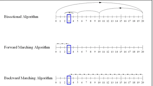
The strength of the bisectional algorithm in its bias neutrality is also its main limitation. While it is wise to select an algorithm that avoids bias against the solution to the problem, it is also wise to promote bias towards the true solution. Consider the following example: a number is chosen between 1 and 20 inclusive. An algorithm is design to find the number chosen. Suppose that some information about the selection process is known, and it is known that lower numbers are chosen most often.
Three algorithms could be proposed: the bisectional algorithm, the forward marching algorithm, and the backward marching algorithm. As seen from Figure 2.1, the bisectional algorithm performs well with no bias, and solves after six samples. The forward marching algorithm takes advantage of the knowledge that numbers are typically selected from the lower end of the range, and is biased towards the lower numbers. The problem is solved in three samples: twice the efficiency of the bisectional algorithm.
8
Figure 2.1: Comparison of algorithm bias. The bisectional algorithm has no bias, while the forward and backward marching algorithms have bias towards lower and higher numbers, respectively.
The backward marching algorithm opposes the known information, and is biased towards the higher numbers. Coincidentally, the problem solves after seventeen samples: almost one third of the efficiency of the bisectional algorithm. In the same manner as this example, the slope stability software can be improved by taking advantage of known information about the problem characteristics.
2.2.2 Analysis of Inefficiencies in Current Software
Two major inefficiencies were found using the bisectional algorithm. The first is the amount of time spent in the non-convergent range, and the second is the small SRF steps in the fully elastic range. 2.2.2.1 Too Much Time Spent in Non-Convergent Range
The finite element software uses a non-linear solver to compute the displacement vector of the element nodes. The non-linear solver uses an iterative technique to converge on a deformed slope shape. If the iteration ceiling is reached, it suggests that the matrix does not have a physical solution and thus we enter the non-convergent range. One important property of the non-linear solver is that each individual iteration within the solver, involving just forward and back-substitutions, requires approximately the same amount of time and computer resources as any other iteration. Practically, this means that more iterations before convergence requires more time, and that non-convergent samples take the most time to calculate.
9
Since the bisectional algorithm does not distinguish between samples that are solved in two iterations and samples that reach the iteration ceiling, it neither avoids the non-convergent range nor favors the convergent range. The result is perhaps more time than is necessary spent in the non-convergent range where Strength Reduction Factor trials take longer to compute. A well-designed algorithm for this software would address this issue by minimizing the number of samples taken in the non-convergent range.
2.2.2.2 Small SRF Steps in the Elastic Range
Within the convergent range of the finite element slope stability method, there are two regimes. The first is the elastic regime where no element in the model is loaded past the yield strength. The second is the plastic regime, where individual elements undergo plastic deformation, but where surrounding elements are able to take the added load and prevent global failure. If all elements along the slip plane underwent plastic deformation, then the model would enter the non-convergent plane.
Since the elastic regime is comprised of only elastic deformations, and since elastic deformation is governed by a linear equation, the solver is very efficient at solving problems in the elastic regime, reaching convergence in one iteration and detecting convergence in two. More important to algorithm design is the fact that slopes tend to have a sizeable plastic regime, so trial Strength Reduction Factors in the elastic regime are buffered from the non-convergent range. In essence, we can afford to use a larger SRF advancing step in the elastic regime than in the plastic regime. While less important than avoiding the non-convergent range, a well-designed algorithm would be able to use larger advancing steps in the elastic regime than in the plastic regime.
2.3 Development of a New Algorithm
This section explores the development of the algorithms presented for incorporation to the slope stability software. The algorithms in this section are presented in the same order that they were considered for use by the author. Many of them were rejected after initial testing and thus do not appear in the parameter optimization or final program development sections.
2.3.1 Curve Fitting
The first breed of algorithms proposed fall into the class of curve-fitting algorithms. These algorithms assume a shape of the modeled function and adjust parameters to match the shape of the model as best as possible. While all of the curve-fitting algorithms presented in this research are also bounded root algorithms, the main focus of these algorithms is the curve-fitting aspect.
10 2.3.1.1 Linear Fit
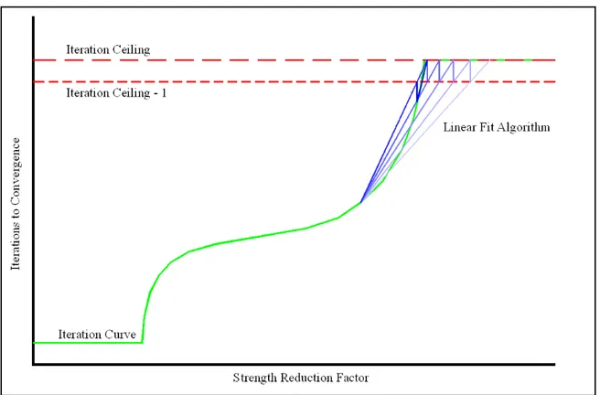
The linear fitting interpolation technique employs the assumption that the model is linear between two sampled points. In the slope stability application, a line is drawn between the highest convergent value of the strength reduction factor and the lowest non-convergent value, and the point at which the line crosses the iteration ceiling minus one, is the sample point. The unit subtraction from the iteration ceiling is meant to address the fact that the number of iterations in the lowest non-convergent value is the iteration ceiling, so without the subtraction the model would sample the same point indefinitely. An example operation of the linear fit algorithm is given in Figure 2.2.
Figure 2.2: Visualization of the linear fit algorithm. The lighter blue lines are the earlier steps of calculation sequence.
In the figure, the linear fit algorithm is depicted by a series of blue lines, with the earlier trials being shaded brighter than the later trials. This example reveals an obvious failure in the algorithm. Because the number of iterations to convergence is clipped to the iteration ceiling, the linear fit algorithm spends nearly all of its time in the non-convergent range, which is exactly what was being avoided. An algorithm was needed that could account for the inflection point at the iteration ceiling.
11 2.3.1.2 Quadratic Fit
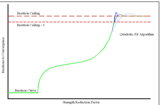
The quadratic fit algorithm was created to address the curvature needs of the solver as previously discussed. It is similar to the linear fit algorithm, except that it assumes a parabolic model shape. It begins by sampling the midpoint between the maximum convergent value and the minimum non-convergent value. With three sample points, the algorithm can now determine the parameters to define a parabola that passes through the three points. The point at which the parabola passes the iteration ceiling minus one becomes the next sample point, and depending on whether the new sample point was convergent or non-convergent, the lowest or the highest of the original three points is dropped and replaced with the new sample point. Figure 2.3 gives an example of this process.
Figure 2.3: Visualization of the quadratic fit algorithm. The lighter blue lines are the earlier steps of calculation sequence.
The quadratic fit algorithm shows improved results against the linear fit algorithm, but it still samples mostly in the non-convergent range. The main problem encountered is that iteration ceiling provides a sharp inflection point, to the extent that the iteration curve becomes non-continuous. It proves inefficient to model a function with infinite curvature using an algorithm that has finite curvature. It can be concluded that an efficient algorithm does not model the shape of the failure point, but perhaps the shape of the convergent range.
12 2.3.1.3 Generalized Curve Fitting Algorithms
An attempt was made to design an algorithm that could predict the factor of safety by sampling the plastic regime of the model’s convergent range. If a generalized function could be found that describes the approximate shape of the plastic regime, then a few points could be sampled to determine approximately where the factor of safety will be.
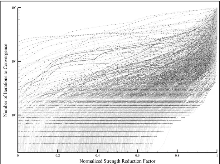
Figure 2.4: Iteration curves for 1000 slopes. The Strength Reduction Factor was normalized to be zero at an SRF of 0.1 and one at the slope’s factor of safety. The iteration curves are widely varied and do not
follow a single curve shape.
It was found, however, that different scenarios followed non-conforming iteration curves. Figure 2.4 shows the iteration curves for the 1000 scenarios used in Section 3.1.1. The strength reduction factor has been normalized such that a normalized strength reduction factor of one is the boundary between the convergent and non-convergent range for a scenario, and a value of zero is the minimum strength reduction factor tested, which was 0.1.
13
With such a wide variety of shapes, it would be overwhelmingly difficult if not impossible to construct a single function to describe the behavior of every curve that could be constructed. It was therefore decided to abandon the curve-fitting algorithms and use a more generic design to construct the finite element slope stability solver.
2.3.2 Bounded Root Algorithms
Bounded root algorithms were briefly described in Section 2.1. They work by subdividing a range that bounds the targeted value until the range is smaller or equal to the tolerance. They are called bounded root algorithms because the typical application is in finding roots of polynomials or other functions. The application of slope stability analysis, however, uses a target value of the iteration ceiling for the upper bound and anything less than the iteration ceiling for the lower bound. The bisectional algorithm implemented in the current software falls into this category, as do the weighted bisectional and FG-Adaptive algorithms.
2.3.2.1 Weighted Bisectional Algorithm
As was discussed in Section 2.2.2.1, the bisectional algorithm is unable to avoid the non-convergent range or to favor the non-convergent range. To help balance the algorithm, a weighting factor was introduced. The weighting factor adjusts the location of the subdividing sample point so that is may not be exactly in the middle of the bounded range. More information about the operation of the algorithm is available in Section 3.2.2.
The mechanism by which the weighting factor improves the performance of the weighted bisectional algorithm can be summarized using the following example. Instead of an elastic and plastic regime, suppose that the model’s convergent range consisted only of an elastic regime. This would mean that strength reduction factors below the factor of safety would all converge in two iterations, and strength reduction factors above the factor of safety would reach the iteration ceiling. If this were the case, it is easily discernable that the convergent range is so cheap in calculating as to be nearly negligible in time and computer resource usage. It would be an obvious advantage to favor the convergent range over the non-convergent range. In fact, it would be so much an advantage that the optimal weighting factor would produce samples that are within the tolerance value so that the non-convergent range does not have to be sampled more than once.
In the actual finite element model, the plastic range creates somewhat of a gradient between two iterations and the iteration ceiling. So there is a weighting factor that is somewhere between zero and one that reaches the optimal balance between fewer non-convergent samples and oversampling the convergent range. Beginning in Chapter 3, this algorithm will be tested and validated for improved efficiency.
14 2.3.2.2 FG-Adaptive Algorithm
The FG-Adaptive Algorithm is an adaptation of the weighted bisectional algorithm that addresses the step size challenge discussed in Section 2.2.2.2. The mechanics of the algorithm are describes in Sections 3.2.3 and 3.4.1.3. In brief, the FG-Adaptive Algorithm uses adaptive stepping to increase the step size in the elastic regime and reduce the step size in the upper plastic regime.
The reduction of the step size is determined by the kernel, which is a function of the number of iterations to convergence and the iteration ceiling. On a conceptual level, reducing the strength reduction factor advancement step size can be compared to a vehicle stopping at a stop sign. As the vehicle approaches the stop sign, the driver observes the upcoming sign and begins to apply the brake, thereby reducing the speed of the vehicle. While slowing, the driver continuously reevaluates the effect of the brake on the speed of the vehicle, as well as the remaining distance to the stop sign. The vehicle eventually comes to a stop immediately in front of the stop sign. In the same manner, the FG-Adaptive algorithm detects the upcoming non-convergent range and reduces the step size in an attempt to capture the factor of safety with as little overshooting and bisecting as possible. As with the weighted bisectional algorithm, the FG-Adaptive Algorithm will be tested and validated beginning in Chapter 3.
15
CHAPTER 3
DETERMINING ALGORITHM PARAMETERS AND MEASURING EFFICIENCY
As with the numerical model itself, the various algorithms considered for implementation must first be calibrated and then tested and validated to ensure that improved performance has been reached. The calibration was carried out using a batch of test scenarios.3.1 Test Scenarios
A test dataset of 1000 slope scenarios was created to compare the performance of the Adaptive algorithm against the original bisectional algorithm, and to optimize the performance of the FG-Adaptive algorithm.
3.1.1 1000 Randomly Generated Scenarios
A large dataset was desired for testing and optimization for the following reasons. First, the use of a large dataset in optimization allows for good overall performance of the algorithm across a wide range of slopes, rather than optimizing for a single slope and having poor performance otherwise. Second, a large dataset allows for the gauging of algorithm sensitivity to scenario variations. A good performance with little variation among scenarios suggests a stable and efficient algorithm, while large variations in performance among the different scenarios might suggest instability and conditional improvements in program performance.
The dataset was created using random input parameters for each scenario. Scenarios varied in their physical dimensions, mesh fineness, soil properties, drained or undrained condition, soil distribution, and model parameters as shown in Table 3.1. The random parameters and their allowable ranges were designed to capture a wide variety of slopes while limiting the number of unrealistic scenarios.
These 1000 slope scenarios would eventually be run through a Monte Carlo simulator to optimize the algorithm parameters. This optimization simulator will be described in detail hereafter. There existed a strong probability that upwards of one million Monte Carlo simulations would be run for each slope scenario to perform adequate optimization on the algorithms. Supposing that 1000 slope simulations needed to be run under different algorithm parameters one million times each, one could easily see that one billion simulations must be run altogether. Considering that the average scenario took about 15 minutes to solve on a standard desktop computer, it would take on the order of 28,000 years to solve all simulations (which would make for a delayed thesis completion indeed).
16
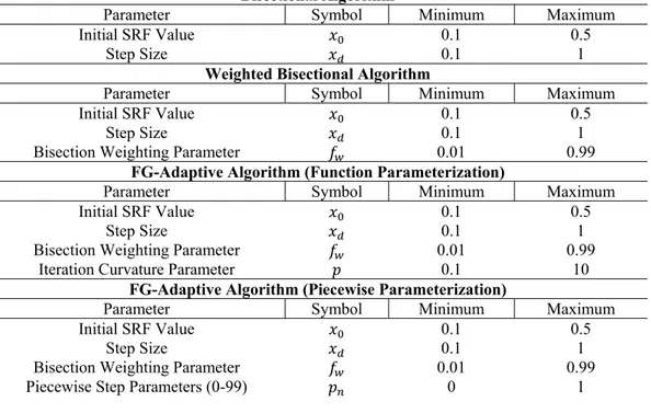
Table 3.1: Optimization parameters for each algorithm, and parameter optimization ranges. Bisectional Algorithm
Parameter Symbol Minimum Maximum
Initial SRF Value 0.1 0.5
Step Size 0.1 1
Weighted Bisectional Algorithm
Parameter Symbol Minimum Maximum
Initial SRF Value 0.1 0.5
Step Size 0.1 1
Bisection Weighting Parameter 0.01 0.99
FG-Adaptive Algorithm (Function Parameterization)
Parameter Symbol Minimum Maximum
Initial SRF Value 0.1 0.5
Step Size 0.1 1
Bisection Weighting Parameter 0.01 0.99
Iteration Curvature Parameter 0.1 10
FG-Adaptive Algorithm (Piecewise Parameterization)
Parameter Symbol Minimum Maximum
Initial SRF Value 0.1 0.5
Step Size 0.1 1
Bisection Weighting Parameter 0.01 0.99
Piecewise Step Parameters (0-99) 0 1
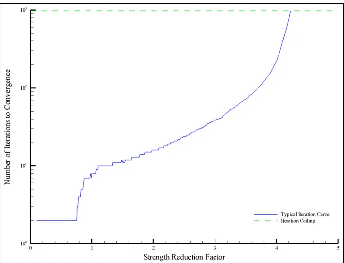
An alternative to 28,000-years of research is to determine the number of iterations and the maximum nodal displacement for all SRF’s between 0.10 and 5.00 in increments of 0.01 to generate an iteration curve for each scenario. An example of such a curve is given in Figure 3.1. Once the curves are created for each scenario, the Monte Carlo optimization can be accomplished in a fraction of the time by estimating the number of iterations to convergence or the maximum nodal displacement for any SRF. This is done by looking up the values off of the iteration curve.
After generating the iteration curves for each scenario, the curves were checked for unrealistic scenarios. For the purposes of this thesis, an unrealistic scenario is one that fails to converge before a SRF of 0.30 is reached, or a scenario that fails to converge after a SRF of 5.00 is reached. In one case the slope is too unstable to be considered well-posed, and in the other the slope is too stable to be well-posed. Of the 1000 scenarios, 362 were rejected because they were ill-posed, leaving 638 scenarios to be included in the algorithm testing and optimization.
3.1.2 Subsets of Interest
The random scenarios were created with particular attention to the following subsets. These subsets were identified to delineate groups of slopes that might behave similarly. If the slopes in these groups show like behavior, then the algorithm could be tuned specifically for that class of problem.
17
Figure 3.1: Typical iteration curve. The iteration curve has a sharp increase of iterations to convergence starting with a Strength Reduction Factor of 4.0.
3.1.2.1 Shallow Slope (Constructed Slopes)
Shallow scenarios have a slope between 0.2 and 1.0. This class is meant to represent engineered, or constructed slopes such as those in channels or along roadways. Of the 638 well-posed scenarios, 298 were shallow slope scenarios.
3.1.2.2 Steep Slopes (Natural Slopes)
Steep scenarios have a slope between 1.0 and 5.0. This class represents natural slopes such as mountainsides and faults. There were 340 well-posed steep slope scenarios.
3.1.2.3 Undrained Slopes
Undrained slopes are a particular interest in slope stability analysis because they represent the transient aspect of slope loads. An undrained condition usually occurs when a clay soil is loaded suddenly and water is not given time to escape the soil. The result is changes in water pressure in the soil (Duncan
18
and Wright, 2005). Undrained slopes are modeled with a friction angle, phi, equal to zero. There were 300 well-posed undrained scenarios.
3.1.2.4 Drained Slopes
Drained slopes capture the steady-state aspect of slope stability. In clay, once the water has time to drain its excess pressure, it enters a drained condition. Sands and gravels do not typically enter an undrained condition. There were 338 well-posed drained scenarios.
3.1.2.5 Homogenous Slopes
Homogeneous slopes have no spatial variability in soil properties. This makes their failure mode and shape more predictable than heterogeneous slopes. There were 214 well-posed homogeneous slope scenarios.
3.1.2.6 Layered Slopes
In this analysis, layered slopes refer specifically to horizontally layered slopes. Each slope was modeled with somewhere between 2 and 7 (inclusive) layers. There were 196 well-posed layered slope scenarios.
3.1.2.7 Randomly Distributed Slopes
Randomly distributed slopes were meant to test the robustness of each algorithm. Since these behave the least predictably of all the slopes, they were meant to represent the most difficult problems for these algorithms to solve. There were 228 well-posed randomly distributed slope scenarios.
3.2 Algorithms Tested
As a discussion on the calibration of several algorithms begins, it is fitting that the behavior of each algorithm be explicitly described to better illustrate the need for calibration in the first place. These include the Bisectional, Weighted Bisectional, and the FG-Adaptive algorithms.
3.2.1 Bisectional
The bisectional algorithm is currently deployed in the Finite Element Slope Stability model. It is tested to provide a reference for the other tested algorithms. The model starts at , where is the first trial strength reduction factor. The algorithm then advances the strength reduction factor as follows:
Where is the standard step size for advancing the strength reduction factor. Once non-convergence is reached, the algorithm switches to the following formula:
19 2
Where is the lowest non-convergent solution (the upper bound of the factor of safety) and is the highest convergent solution (the lower bound of the factor of safety). The model completes once
is smaller than the tolerance specified as an input to the model. 3.2.2 Weighted Bisectional
The weighted bisectional algorithm is a slight variation on the current bisectional algorithm. This algorithm is included to test the performance improvements available without designing an algorithm custom to the slope stability application. It will enable the author to measure the improvements of the FG-Adaptive Algorithm above commonly used accelerators.
The weighted bisectional algorithm is similar to the bisectional algorithm. Like the bisectional algorithm, the weighted bisectional algorithm begins at
, where is the first trial strength reduction factor. Also the same is the method for advancing the strength reduction factor:
Where is the standard step size for advancing the strength reduction factor. However, once non-convergence is reached, the algorithm switches to a different formula:
Where is the lowest non-convergent solution (the upper bound of the factor of safety), is the highest convergent solution (the lower bound of the factor of safety), and is the weighting factor for the model. The model completes once is smaller than the tolerance specified as an input to the model.
3.2.3 FG-Adaptive (Function Parameterization)
The FG-Adaptive Algorithm is designed specifically for use in the Finite Element Slope Stability model. Like the bisectional and weighted bisectional algorithms, this algorithm begins at
,
where
is the first trial strength reduction factor. A standard step size is defined for
advancing the strength reduction factor, but the algorithm reduces the actual step taken as the
number of iterations to convergence increases, so that
, ,
Where is the number of iterations to convergence and is the iteration ceiling. For the function parameterization of the FG-Adaptive Algorithm, , , is:
20
, , 1 log
log
If , , evaluates to a value smaller than one half the tolerance then one half the tolerance is used.
In the event that the model fails to converge, the algorithm uses the following formulas:
, ,
Where is the weighting factor for the model and is the highest convergent solution (the lower bound of the factor of safety). Once is reduced, it remains at its reduced value until either the model completes or until it is further reduced. Unlike the bisectional and weighted bisectional algorithms, the FG-Adaptive Algorithm uses the first equation as often as convergence is reached for a given strength reduction factor, even if it is after non-convergence is reached for the first time.
The model completes once is smaller than the tolerance specified as an input to the model. 3.2.4 FG-Adaptive (Piecewise Parameterization)
The piecewise parameterization of the FG-Adaptive Algorithm is identical to the function parameterization, except that , , is more generally defined than in the function parameterization:
, , ; log
log
Where is the number of iterations to convergence, is the iteration ceiling, is the standard step size for advancing the strength reduction factor, and is a set of parameters that represent the diminishing of the strength reduction factor advancement as the number of iterations to convergence approaches the iteration ceiling. Each parameter has a value of
0 1
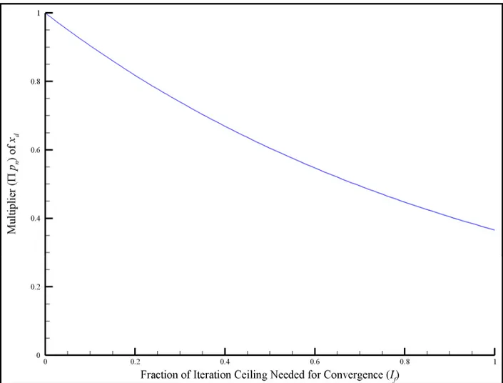
If all ’s are 1 then the algorithm does not reduce the strength reduction factor step size. Figure 3.2 shows the case of all ’s having a value of 0.99. The piecewise parameterization of the FG-Adaptive Algorithm was introduced to detect any limitations to the function parameterization caused by the pre-defined curvature of , , .
21 3.3 Optimizing Parameters
Several of the variables in each algorithm listed in Section 3.2 were designated as algorithm parameters to be varied to optimize the performance of each algorithm. These variables are summarized in Table 3.1.
Figure 3.2: Function kernel , , of the piecewise FG-Adaptive algorithm when every is set to 0.99.
3.3.1 Monte Carlo Simulator to Optimize Parameters
A Monte Carlo simulator was written to perform the parameters optimization. This program accepts all iteration curves for any one scenario set and estimates the performance of the finite element slope stability software using each algorithm. Each optimizing parameter is assigned a random value within a predefined range specific to that parameter. For example, the weighted bisectional algorithm has a weighting factor, which is randomly assigned values between 0 and 1 for each perturbation. The measure for algorithm performance is the total number of iterations to model completion. This means that
22
the number of iterations to reach convergence is summed over all the strength reduction factors until the model completes for each scenario. This total is summed over all scenarios to get the algorithm performance measure.
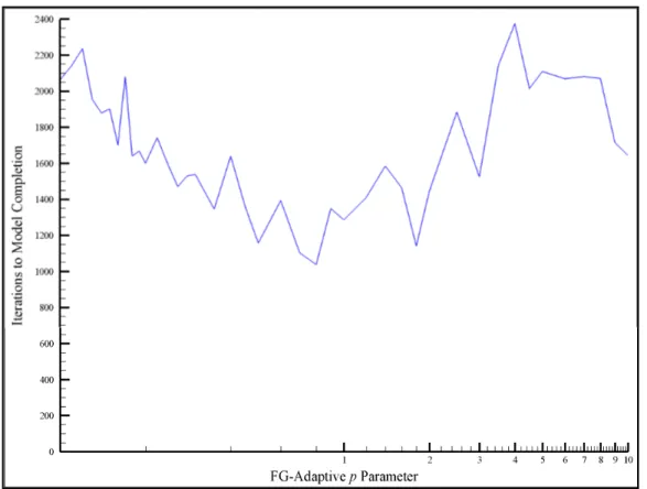
10,000 perturbations were generated, and the Monte Carlo results were loaded into a database and queried for the optimal parameter ranges. It was found that the ranges were much too wide to produce meaningful optimization. This behavior is found when a parameter creates any sort of sinusoidal behavior in the model (such as the performance of the FG-Adaptive algorithm with the power parameter swept across its range as shown in Figure 3.3). Therefore, a different optimization technique from Monte Carlo was used.
Figure 3.3: Iterations to completion for a sample slope swept across the power parameter range.
3.3.2 Brute-Force Simulator to Optimize Parameters
Another common non-linear solver is a brute-force simulator, using a one-factor-at-a-time solving technique. This kind of technique is common in sensitivity analyses. In this implementation of the one-factor-at-a-time brute-force simulator, all optimizing parameters are given an initial value and are, one at a time, swept across the range specified for that parameter. The value that produces the best performance in the algorithm is assigned back to the parameter. Each parameter is tested until all have been optimized.
23
Once all parameters have been optimized in the manner described above, the simulator will recursively re-optimize each parameter in succession until two recursions produce the same algorithm performance. A thorough explanation of the program is given in Section 3.3.3 and a copy of the codes is available in Appendix B.
This method performs quite well when there are relatively few parameters, and when the output is a relatively smooth function of the input parameters. When there are a large number of input parameters or when the output is a severely non-linear function of the input parameters, the brute force method may find a local minimum without finding the absolute minimum number of iterations given the parameter ranges. In the brute-force results, this local-minimum phenomenon appears occasionally. Fortunately, there are two versions of the FG-Adaptive Algorithm where this phenomenon is most often observed: the function definition and the piecewise definition. Typically at least one of the algorithm versions finds a solution that indicates model performance improvements.
Several measures were used to determine algorithm performance improvement potential. First, the total number of iterations to model completion was summed across all scenarios and then divided by the number of scenarios in the scenario set to obtain the average performance of each algorithm. This will be referred to hereafter as Average Total Iterations. By optimizing the Average Total Iterations, each algorithm can perform its best when calculating the factor of safety for a selection of multiple slopes. Some slopes will take longer to solve and others will solve with very few total iterations. But overall, each algorithm will be tuned for best long-term performance. The second measure was the maximum of the total number of iterations to model completion across all scenarios in a set. The third measure is closely correlated; the third measure is the 97.5 percent one-sided upper confidence limit of the total number of iterations to model completion across a scenario set (Navidi, 2011). By using the upper confidence limit, extreme outliers are ignored and the general performance for any one simulation is ascertained. In both the Maximum Total Iterations and the UCL Total Iterations, the algorithm optimized to perform efficiently for any single scenario without calibrating the model parameters to that scenario explicitly. This is useful when only one or a few scenarios are considered, and the averaging effects of multiple scenarios are negated. The final measure is that of calibrating to a single scenario randomly selected from the scenario set. By using only one scenario, we can measure the ability of an algorithm to adapt to a problem and obtain a factor of safety in a minimal number of iterations.
3.3.3 Building the Program to Optimize the Algorithm Parameters
A program was developed to automate the parameter calibration process. This software was designed both to efficiently automate the calibration processes described in Sections 3.3.1 and 3.3.2, and to allow for easy future development of algorithms. The software was written in Visual Basic, which is
24
preferable to FORTRAN when flexible programming takes higher priority than computational speed. The major advantage of Visual Basic is the object-oriented capabilities of the language. A thorough discussion of the use of classes and objects in the software can be found in Appendix B.
3.3.3.1 Program Design
The design features of the software that are of interest outside the scope of the programmer can be summarized thus:
• Simulating the Slope Stability software from the iteration curves • Calculation of the optimization measure
• The optimization process
The slope stability program is not ever actually run during optimization. As explained in Section 3.1.1, an optimization process that runs the slope stability code for each scenario and each Monte Carlo iteration would require unrealistic computer resources and processing time to complete. Instead, the result files from the 638 well-posed randomly generated scenarios were read into the optimization software to construct the iteration curves. The iteration curves were then used as a reference for simulating the slope stability software performance for each scenario. The test algorithm would select a trial SRF and lookup the number of iterations to convergence off the iteration curve. The number of iterations determined what the next action of the algorithm was. And so the algorithm would select a new SRF and lookup a new number of iterations. Eventually, the bounded region where the factor of safety is possible would be smaller than the tolerance on the factor of safety and the model would be complete.
The software tracks the total number of iterations to model completion for each scenario. After completing all scenarios in the scenario batch, the model can report nearly any statistic of the iterations for the batch. In this research, the average, maximum, 97.5 percent UCL, and the number of iterations for a single scenario were reported to capture various aspects of the dataset’s behavior.
Optimization occurs either by running Monte Carlo perturbations or by sweeping through the algorithm parameter ranges looking for the value that produces the lowest optimization measure. In both cases, the optimizing parameters as shown in Table 1 are assigned and then all scenarios in the batch are simulated. An optimization measure is outputted and the program uses that data to help determine the next perturbation.
3.3.3.2 Flexible Design for Future Work
It is recognized that this thesis marks the beginning, not the end, of algorithm optimization for the Finite Element method on slope stability analysis. It was therefore of upmost interest to design the optimization software for use in future algorithm development.
25
The main feature of the program that allows for future algorithm development is the use of inherited classes. Inherited classes have two parts. First is the class signature, described as a MustInherit class. The MustInherit class tells the program what all Inherits classes will look like to the rest of the program in regards to function and subroutine signatures. The Inherits classes then describe the processes that go into each function and subroutine to generate the needed output.
This may seem like an abstract concept, but can be illustrated easily using the following example. Consider a USB port on the front of a computer. The USB port has certain dimensions and power requirements for all devices that use the port. A multitude of devices ranging from keyboards and mice to jump drives and joysticks have been designed to interface with a USB port. In the same way, the MustInherit class describes the program equivalent of port specifications, and the Inherits class describes the software equivalent of the device itself.
In the optimization software, the MustInherit class is called Algorithm. All Algorithm classes must have certain functions including a SetParameter function and a Solve function. Four Inherits classes are implemented: BisectionalAlgorithm, WeightedBisectional-Algorithm, FarnsworthFunctionWeightedBisectional-Algorithm, and FarnsworthParamAlgorithm. Each of these Inherits classes have the needed functions, but each class has specialized instructions that apply only to that algorithm.
The benefit of this program design is that additional algorithms may be added and tested simply by defining a new Inherits class and then implementing it in the main code. All other program operations automatically connect to the new algorithm.
3.3.3.3 Data Management
The data generated by 638 scenarios and 10,000 perturbations using four algorithms each with several optimizing parameters can be taxing if not fatal to the system if not handled properly. To avoid running out of memory while maintaining quick access to the data, a database was designed to store the various aspects of the optimization runs. This database is referred to in the code in Appendix B, and is needed to run the optimization software. A brief description of the database schema is given in Appendix C, and is also included in the computer files in Appendix D.
3.3.4 Determination of Optimal Parameters
The optimized parameters and the selection of the most efficient algorithm are shown in Table 3.2. Under the Average Total Iterations measure, the FG-Adaptive Algorithm was shown to perform the best out of the tested algorithms in all scenario sets except for the shallow undrained homogeneous slope set. The FG-Adaptive Algorithm would then be the algorithm of choice when modeling several scenarios in batch. Meanwhile, the Weighted-Bisectional algorithm regularly out-performed the FG-Adaptive
Table 3.2: Summary of f optimized pa
26
27
algorithm when optimizing for Maximum or UCL Total Iterations. This implies that the FG-Adaptive Algorithm is on average more efficient than the Bisectional and the Weighted Bisectional Algorithms, but that the FG-Adaptive Algorithm is more sensitive to each individual problem and therefore has a wider variance. The Single-Scenario measure casts some additional light on the capabilities of the various algorithms. This measure does not carry any sort of weighting or averaging effect. It simply tries to optimize an algorithm to a single curve. What has been shown is that the Weighted Bisectional Algorithm generally performs twice as efficiently as the Bisectional Algorithm, and that the FG-Adaptive Algorithm performs about twice as well as the Weighted Bisectional Algorithm. This means that, while it is beyond the scope of this research, if the FG-Adaptive Algorithm can be calibrated to the slope in question, then that algorithm can perform about three times as quickly as the current software implementation.
Some of the optimized parameters were not used in the final implementation of the software. Instead, they revealed weaknesses in the design of the algorithm or the optimization process. These parameters, the weaknesses revealed, and the actions taken to address the issues are summarized in Section 3.4.
3.4 Final Program Development
After calibration came the implementation of the final FORTRAN code for finite element slope stability analysis. In addition to the optimal parameter values, several other discoveries were made during calibration that led to a final implementation of the algorithms of interest.
3.4.1 Lessons Learned from Parameter Optimization
Three important lessons were learned from parameter calibration, two of which led to slight algorithm design modifications. These modifications dramatically improved algorithm performance, and were adapted into the code used for the case studies in Chapter 4. The code available in Appendix A is the final code with all changes implemented.
3.4.1.1 Lesson 1: Bisectional Algorithm Step Size
In Dr. Griffiths’s Slope Stability software, the strength reduction factor step size is fixed at ten times the inputted tolerance on the factor of safety. During parameter optimization, however, both the bisectional algorithm and the weighted bisectional algorithm consistently found the optimal strength reduction factor step to be 0.15. The frequency and regularity of that number was the cause of some investigation into the mechanics of the bisectional algorithm. From that investigation came the uncovering of a basic mathematical principle that operates heavily in the bisectional algorithm. Simply stated the principle in operation is:
28
In practice, this means that the strength reduction factor step is approximately 24 times the tolerance on the factor of safety. Considering that fact that the bisectional algorithm divides by two to narrow the range of possible slope failures, it makes perfect sense that the optimal step size would be some power of two multiple of the tolerance. In implementation, the number has to be slightly smaller to account for finite precision on a computer. So the number one lesson learned was why the optimal step parameter value was 0.15.
3.4.1.2 Lesson 2: Weighting Factor
In parameter optimization, the weighted bisectional algorithm was given 0.25 as the optimal bisection weighting parameter value. However, it was found that the value of that parameter was too small to perform well in practice. The main reason for the poor performance is likely that the optimization scenarios were randomly created, and many of the slopes had small factors of safety. These slopes may have skewed down the bisection weighting parameter value.
Slopes with small factors of safety have a particularly profound effect on the weighting factor because of the nature of their iteration curves. The bisection weighting parameter tries to capture the fact that it is slightly less expensive on computer resources to calculate a convergent solution than it is to hit the iteration ceiling. The lower the number of iterations is near the model’s factor of safety, the more advantageous it is to stay in a convergent range, and so the bisection weighting parameter value tends to lower values. Likewise, when the number of iterations near the model’s factor of safety is close to the iteration ceiling, there is little advantage to staying in the convergent range, and so the bisection weighting parameter value tends towards 0.5. Since the scenarios with low factors of safety had more compressed iteration curves and therefore lower iteration numbers near the model’s factor of safety, they tended to skew the bisection weighting parameter down. To correct for this, the bisection weighting parameter value was changed from 0.25 to 0.40.
3.4.1.3 Lesson 3: FG-Adaptive Algorithm Step Control
Two efficiency problems were observed in the FG-Adaptive algorithm. The first problem was that the curvature parameter, p, was unable to fit the iteration curve. If the curvature parameter was set to a lower number, the automatic step control would perform well until the number of iterations to convergence approached the iteration ceiling. Then the algorithm would consistently overshoot the model’s factor of safety. It the curvature parameter was set to a higher number, then the model would not reduce the strength reduction factor enough in the low-iteration-convergence range and the model would step over the higher-iteration-convergence range by its large step and overshoot the factor of safety. To address this problem, the function kernel in the algorithm was modified to reach the minimum step size when the number of iterations reached half the iteration ceiling. In most scenarios, by the time the model
29
took half the iteration ceiling to converge, it was within about 0.02 of the model’s factor of safety. This modification allowed the model to maintain the efficient automatic step control in the lower-iteration-convergence range, while creating a sharp reduction in step size in the higher-iteration-lower-iteration-convergence range.
The second issue was that when the algorithm overshot more than once or twice, the step size was reduced to below the factor of safety tolerance. The algorithm originally included a minimum step size filter to ensure that the smallest step was at least half the tolerance on the factor of safety. However, it was decided that the filter was set too tight, and that using the full tolerance (minus a small proportion to address finite precision) does not adversely affect the algorithm output. Therefore, the filter was changed accordingly. Additionally, the SRF step kernel was adjusted to produce a minimum value of the tolerance (again, minus a small proportion to address finite precision) to reduce how often the algorithm relied on the filter.
In summary, the following changes were made to the algorithm:
, , 0.9 1 min ,
log 0.9
If , , evaluates to a value smaller than 90% of the tolerance then 90% of the tolerance is used.
3.4.2 Programming the Algorithm in FORTRAN
Up until this point, all three algorithms under consideration only existed as procedures in the parameter optimization software that sampled an iteration curve and returned the theoretical number of iterations to model completion. The algorithms needed to be coded into a form that can be incorporated into the slope stability simulation software to allow for functional testing and use of the software. One of the major goals of the coding was to place as few of edits in the original software as possible, thus maximizing the amount of code that is placed in a separate algorithm subroutine.
The main software adaptation is nearly identical among the three algorithms, with the only significant difference being that the FG-Adaptive Algorithm reads in a few extra values in the input file and stores a couple more variables in the main program. Otherwise, the algorithm is housed completely in the algorithm subroutine. For the bisectional algorithm, the subroutine is algbis. The weighted bisectional algorithm subroutine is algwbs, and the FG-Adaptive algorithm is algfga.
Appendix A contains four versions of Program 6.4 from Programming the Finite Element Method (Smith et al., 2014). The first version is the software as presented in the book, in which the user specifies the strength reduction factors to test. The other three versions of the code are embedded with the three algorithms.
30
As a note, Program 6.4 is a simplified version of the software described in Griffiths and Lane, 1999. Among other features, Program 6.4 does not contain the bisectional algorithm that is included in the full software version. Since the bisectional algorithm was also optimized in this research, the version of the code in Appendix A that includes the bisectional algorithm uses the optimized bisectional algorithm, not the bisectional algorithm used in Griffiths and Lane, 1999. The bisectional algorithm used in the case studies in Chapter 4 is also the optimized bisectional algorithm.
31
CHAPTER 4
CASE STUDIES
Five case studies were examined to demonstrate the improvements in software performance by the weighted bisectional and the FG-Adaptive algorithms. The slopes for these case studies were taken from a variety of sources that examine realistic slopes.
4.1 Case Study 1: Shallow Homogeneous Undrained Slope
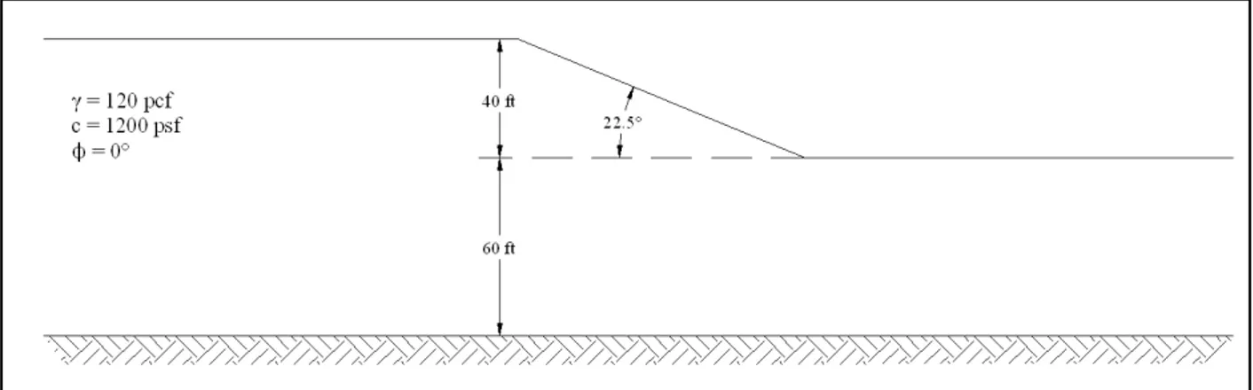
A slope was analyzed by Huang (2014) using the Taylor (1937, 1948) stability chart for soils with a friction angle of zero. A cross section of the slope is provided in Figure 4.1. Using the chart, a Factor of Safety of 1.46 was calculated.
Figure 4.1: Slope geometry and geology recreated from Huang (2014), Figure 7-2.
The slope as also analyzed using the Finite Element Method. Figure 4.2 shows the un-deformed mesh, and Figure 4.3 shows the failed, deformed mesh. The Finite Element Method produced a Factor of Safety for the slope of 1.43, which is in close agreement with the Factor of Safety estimated from the chart.
Figure 4.3 shows only a portion of the failure mechanism. To ensure that the slope had actually failed, the finite element method was rerun with an iteration ceiling of 1000 iterations instead of the default 500. Figure 4.4 shows the deformed mesh. It is clear that after 1000 iterations the failure shape is more developed than after 500. This brings up the question of how high the iteration ceiling needs to be to reliably capture slope failure. If the iteration ceiling is too low, it might terminate the run prematurely and