Comparing Snowpack Surface Roughness Metrics with a
Geometric-based Roughness Length
S.R. Fassnacht
ESS-Watershed Science, Colorado State University, Fort Collins, Colorado 80523-1476 USA
I. Oprea and G. Borleske
Mathematics, Colorado State University, Fort Collins, Colorado 80523-1874 USA
D. Kamin
ESS-Watershed Science, Colorado State University, Fort Collins, Colorado 80523-1476 USA
Abstract. The snow surface is the interface between the atmosphere and the earth. It is very dy-namic, and varies spatially and temporally. Its roughness influences turbulence and is used to esti-mate the sensible and latent heat fluxes to and/or from the snow surface to the atmosphere. We use airborne lidar-derived snow surface measurements from the NASA Cold Land Process Experiment Fraser Alpine intensive study area (ISA) collected in late March 2003. A meteorological tower was centered in the middle of the 1 km2 ISA and meteorological data were used to determine the
domi-nant wind direction. The raw surface elevation data were rotated to yield a 100 by 100m area about the tower, that was parallel to the wind. The data were interpolated to a 1-m resolution using four methods to purposefully derive four different snowpack surfaces. Roughness metrics, including the random roughness, autocorrelation, and fractal dimension were computed, and compared to the ge-ometric-based roughness which was derived using the Lettau formulation.
1. Introduction
The extent and duration of seasonal snow cover plays an important role in determining local, regional, and global climates, due to its contribution to the radiation balance of the Earth system and its role in the hydrological cycle. Since the snow surface is the interface between the atmosphere and the earth, understanding changes its characteristics can im-prove our knowledge of hydrologic processes. The aerodynamics of wind movement across a snow surface impacts the climatology of the environment; as a negative conse-quence sublimation losses can increase and available water resources can be reduced.
Snow surface roughness characteristics influence energy exchange, heat transfer, melt-ing in the snowpack, and thus are important input variables in snow-hydrologic models [Herzfeld et al., 2003]. It is also an important factor for the scattering of light and thereby related to the surface albedo, which is one of the essential climate variables (ECV) defined in the Implementation Plan for the Global Observing System for Climate in support of the United Nations Framework Convention on Climate Change (UNFCCC;
<http://unfccc.int/>) (see [Manninen et al., 2012] and references therein).
The surface of the snowpack changes over the winter. The surface roughness can in-crease or dein-crease during snow accumulation as the snow follows the underlying terrain in the initial stages of accumulation [Davison, 2004]. Alternatively, the snowpack surface can change due to redistribution with extreme features, such as sastrugi formed in wind-swept areas. During snowmelt, large roughness features can form and persist throughout the melt period. Rain-on-snow events can generate near surface runoff that can create roughness rills down slopes. The geometry of a snow surface can undergo dramatic temporal changes
that influence climate and hydrology. Therefore, accurate estimates of roughness are need-ed.
Once surface data have been measured, various surface-roughness describing parame-ters and measures are developed to describe roughness (see [Dong et al., 1992, 1993, 1994 a,b] for a review), and the proper choice depends on applications. Several metrics have been used to study the roughness of the snowpack surface from digital imagery [Fassnacht
et al., 2009 a,b], but no comparison has been made between these metrics and the
geomet-rically computed surface roughness length (z0) of the snow, a critical roughness parameter
whose prediction is of fundamental importance for estimating turbulent fluxes since this parameter enters in all existing numerical models of surface-atmosphere interaction. In the present work we compare these metrics with the surface roughness length z0, on the same set of data. We use airborne light detection and ranging (lidar) estimates of the snowpack surface elevation. These elevations are at an approximate resolution of 1.3-m and have been interpolated to a 1-m resolution with four different methods to yield four sets of sur-faces.
2. Background
2.1 Roughness Length
The surface roughness length is governed by roughness and is an important parameter in many surface and climate-related processes. Surface roughness length has been effec-tively used to assess the aerodynamic properties of sandy, vegetated, urban, snow and wa-ter surfaces, and has a direct impact on meteorological models, through its influence on atmospheric turbulence. A rough surface will enhance turbulence and increase atmospheric transfer rates over that surface, but reduce aeolian transport. Although z0 is a critical
varia-ble for estimating surface (latent and sensivaria-ble) fluxes in numerical models, most land sur-face models treat z0 as a function of land cover type and usually assume it is constant over
time for non-vegetated surfaces. For example, one of the more complex land surface schemes, the Community Land Model version 4.0 (CLM4.0), applies a single z0 value of
2.4 x 10⁻³ m to snow-covered surfaces.
Yet, z0 has been reported to vary by orders of magnitude from 0.004 to 30 x 10-3 m for
a variety of snow-covered glaciers [see Brock et al., 2006]. At any specific location, the physical roughness of the snow surface changes over the season [Fassnacht et al., 2009a]. The implication of variability in z0 was tested using a simple bulk transfer formulation for
the latent mass flux; by altering z0 as a function of snow accumulation-settling or
consider-ing directionality of the wind - sublimation estimates varied by at least a factor of two [Fassnacht, 2010].
The value of z0 was estimated from the measurement of surficial features [e.g., Lettau,
1969; Munro, 1989]. The dependence of z0 on the size, shape, density, and distribution of
surface elements has been studied using wind tunnels, analytical investigations, numerical modeling, and field observations [Grimmond and Oke, 1999; Foken, 2008]. The lack of a clear formulation for calculating z0 as a function of surface roughness is due to the
com-plexity of surface roughness that exists in nature. There are two approaches available to determine z0 for such surfaces: 1) micrometeorological or anemometric that relies on field
observations of wind turbulence movement to solve for aerodynamic parameters included in the theoretical relations derived from the logarithmic wind profile, and 2) morphometric
or geometric that uses algorithms relating aerodynamic parameters to measures of surface morphometry [Grimmond and Oke, 1999; Foken, 2008]. In this study, geometric methods will be used with a spatially continuous database of the distribution of roughness elements surrounding the site of interest.
The most common geometric approach is simply a function of the height of the ele-ments:
z0 = f0 zH (1),
where zH is the mean height of roughness elements, and f0 is an empirical coefficient
de-rived from observation.
The frontal area index (which combines mean height, breadth, and density of the roughness elements) is defined [Raupach, 1992] as roughness area density (λF) = Ly zH ρel,
where Ly is the mean breadth of the roughness elements perpendicular to the wind
direc-tion and ρel is the density or number (n) of roughness elements per unit area. Lettau (1969)
developed a formula for z0 for irregular arrays of reasonably homogenous elements:
z0 = 0.5 zH λF (2).
Other methods have been developed, especially to consider more regularly-shaped and dis-tributed roughness elements such as buildings in an urban setting [e.g., Counihan, 1971; Macdonald et al., 1998].
2.2 Roughness Metrics
A variety of roughness metrics have been developed to assess the roughness of a sur-face. Three common sets of roughness metrics are the random roughness (RR), auto-correlation (AC), and variogram analysis [see Fassnacht et al., 2009b]. The RR is comput-ed as the standard deviation of the detrendcomput-ed surface. In three-dimensions, a plane (or line in 2-D) is fitted to the dataset and used to remove trends that would otherwise bias the evaluation. These trends may be elevation gradients [e.g., Deems et al., 2006] or due to in-strument/operator systematic biases [Fassnacht et al., 2009b]. The RR does not consider the spatial structure of roughness, except for the influence on detrending. The detrended data are used for the other two methods.
The AC does consider the spatial structure and requires that the data be distributed on a regular interval. In 2-D it is the correlation coefficient of the each point along the curve with respect to the previous point, while in 3-D it is computed along each row and along each column to yield a series of X and Y AC values. In 2-D photographs of the snow sur-face are derived from the contrast with a black board inserted into the snowpack [Fassnacht
et al., 2009b]. A 3-D surface is often derived from (terrestrial or airborne) light detection
and ranging (lidar) that produces a cloud of points that must be interpolated to a regular grid (see section 2.3 for interpolation procedures).
Variogram analysis does not require data to be on a regular interval, but still considers the spatial structure of the snowpack surface. Here the variance in elevation, i.e., surface height, among each pair of locations, i.e., points, in the data cloud as a function of the dis-tance between points. The (semi-)variance is plotted as a function of the (lag) disdis-tance in log-log space and the fractal dimension (D) is computed as 3 minus the power of the best
fit line divided by two [Deems et al., 2006]. This line is fitted up to the lag distance where the change in variance stops; this is scaled the scale break (SB). The variogram analysis can be performed with all data pairs, or can consider the direction of the pairs; Deems et al. [2006] used the main eight compass directions.
2.3 Point Data Interpolation
A variety of statistical methods have been used to map the distribution of snow data (often snow depth measurements). Kriging (KRG) uses the data to develop a variogram; a function is fit to the increasing part of the variogram that is subsequently used to interpo-lated onto a regular grid up to the scale break [Isaaks and Srivastava, 1989]. The inverse distance weighting (IDW) approach weights a data point elevation based on the inverse of the distance from a grid point to that data point using a power. A power of two is often used, taken from laws of physics.
Other standard interpolation methods include triangulation (TIN) and the nearest neighbor (NN) approaches. The TIN, or triangulated irregular network, fits lines between data pairs to establish triangles that each represent a plane that is interpolated to the chosen grid spacing. The selection of the data pairs is optimized using the Delaunay [1934] meth-od to reduce the number of small angle triangles. The NN approach assigns a grid value based on the nearest observed point.
Terrain-based methods to interpolate snow depth determine the most important param-eters that influence the distribution of snow. These paramparam-eters include elevation, slope, as-pect, location (latitude and longitude for geographic coordinates or easting and northing for Universal Transverse Mercator coordinates), and others derived from slope and aspect. Canopy-based parameters, such as canopy density have been used in forested areas. Binary regression trees splits the dataset into two groups based on the dominant parameter and continues to split the sub-sets further into groups until an average value (or elevation) is computed [Elder et al., 1991]. Multi-variate linear regression and general additive models have also been used [López Moreno and Nogués Bravo, 2006]. Erxleben et al. [2002] pro-vides a comparison of snow depth interpolation methods.
3.
Methods
The purpose of this paper is to estimate i) the geometric-based z0 of a snowpack surface
derived from an airborne lidar dataset using the Lettau [1969] method, and ii) the rough-ness metrics (RR, AC, D and SB) for the same surface. These will be compared for regu-lar-spaced surfaces derived from the same dataset, but interpolated using four interpolation methods to re-create the surface.
3.1 Dataset
Airborne lidar snow surface elevation data were collected in early April 2003 across the NASA Cold Land Process Experiment (CLPX) intensive study areas (ISAs)[Cline et al., 2009]. For this study, the Fraser Alpine (FA) ISA was used since the meteorological tower centered in the middle of the 1 km2 ISA was in an alpine area, i.e., not among trees. The
meteorological data [Elder et al., 2009] were used to determine the dominant wind direc-tion. All CLPX data were retrieved from the National Snow and Ice Data Center [Miller, 2004; Elder and Goodbody, 2004].
raw surface elevation dataset. These were rotated to be with the direction of the dominant wind, and a 140 by 140m area was further extracted producing 7712 elevation points. The data were interpolated to a 1-m resolution using KRG, IDW, TIN and NN. These methods were used as they are known produce different maps [Erxleben et al., 2002;
<http://www.goldensoftware.com>]. To further yield variations in the surface, the subsetted data cloud was randomly resampled at 5-m (824 elevations) and 10-m (225 elevations) resolutions. These resampled datasets were interpolated using the four methods. Kriging with the entire data cloud was used as the ground-truth snow surface. Holland et al. [2008] recommended interpolating lidar data to facilitate the computation of z0 from data on a
regular grid.
4. Results
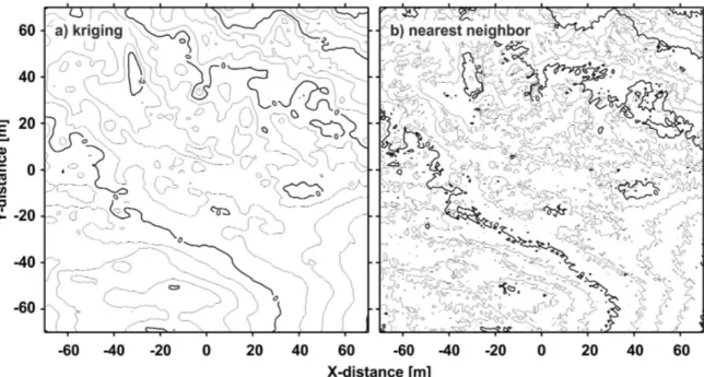
As desired, the four different interpolation methods each produced different snowpack sur-faces. The nearest neighbor interpolation yielded the largest variation (see data range in Table 1; Figure 1) that increased as few data were included in the interpolation. The num-ber of points used in the interpolation decrease from 7712 (raw data) to 824 (5-m subset) to 225 (10-m subset). Assuming that kriging with the raw data produced the best representa-tion of the actual snow surface, the net difference between methods and dataset computed from each of the 19,881 pixels (1m2 interpolation) was small, but the absolute difference was as large as 1.2m (IDW for 10-m subset). Kriging and triangulation produced similar results (Table 1).
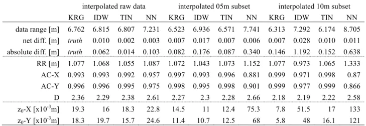
Table 1. Summary of the 12 datasets interpolated using the raw data (~1.6-m resolution), data subset
ran-domly at 5 and 10-m resolutions using kriging (KRG), inverse distance weighting (IDW), triangulation (TIN), and the nearest neighbor (NN) methods. Kriging with the raw data was assumed to be most repre-sentative of the actual snowpack surface and used as the ground truth for comparison of the surfaces. The roughness metrics computed are the random roughness (RR), average autocorrelation (AC) in both the X and Y directions, and the omni-directional fractal dimension (D). The geometric roughness length (z0) was
com-puted using the Lettau method in the X and Y directions.
interpolated raw data interpolated 05m subset interpolated 10m subset
KRG IDW TIN NN KRG IDW TIN NN KRG IDW TIN NN
data range [m] 6.762 6.815 6.807 7.231 6.523 6.936 6.571 7.741 6.313 7.292 6.174 8.705 net diff. [m] truth 0.010 0.002 0.003 0.007 0.017 0.007 0.006 0.007 0.028 0.010 0.011 absolute diff. [m] truth 0.062 0.014 0.103 0.082 0.176 0.087 0.340 0.146 1.192 0.152 0.638 RR [m] 1.077 1.068 1.055 1.087 1.072 1.043 1.073 1.152 1.077 0.973 1.065 1.333 AC-X 0.993 0.993 0.992 0.957 0.997 0.993 0.996 0.881 0.999 0.971 0.998 0.87 AC-Y 0.996 0.996 0.995 0.975 0.998 0.995 0.998 0.901 0.999 0.977 0.999 0.866 D 2.36 2.29 2.38 2.61 2.27 2.3 2.28 2.66 2.18 2.19 2.22 2.58 z0-X [x10-3m] 19.3 16 18.3 22.8 14.5 11 12.4 75.3 7.8 51.5 17 133 z0-Y [x10-3m] 18.3 19.7 15.7 24.6 11.4 10.7 12.5 68 5.8 48 16.1 121
The roughness metrics showed similar patterns (Table 1); as the random roughness in-creased, the autocorrelation decreased and the fractal dimension increased. The fractal di-mension for the nearest neighbor surfaces was the largest as this interpolation method uses the individual data points and there is in essence no smoothing. As the density of data de-creased, D decreased for the other three methods since the surfaces became more regular or
organized (e.g., Fassnacht et al., 2009b). There is directionality in the fractal dimension that is arranged with the wind direction (Figure 2; Deems et al., 2006). Specifically with or parallel to the wind, D is larger and it is small, i.e., more organized perpendicular to the wind.
Figure 1. The snowpack surface derived from the raw data using a) kriging and b) nearest neighbor
methods. For the raw data, the IDW and triangulation surfaces were very similar to the kriged surface (see Table 2). Contours are at 0.5-m intervals with bold lines at 2-m intervals.
Figure 2. The directional variation in fractal dimension (D) for the snowpack surface derived from
the raw data using kriging and nearest neighbor methods, together with the probability of wind blow-ing from a specific direction.
From the raw data, the Lettau geometric roughness was similar for the four methods. For kriging, z0 decreased by half an order of magnitude while it increased by half an order
for NN it increased by half an order of magnitude going to the 5-m subset data and then a factor of 2 further going to the 10-m subset data (Table 1).
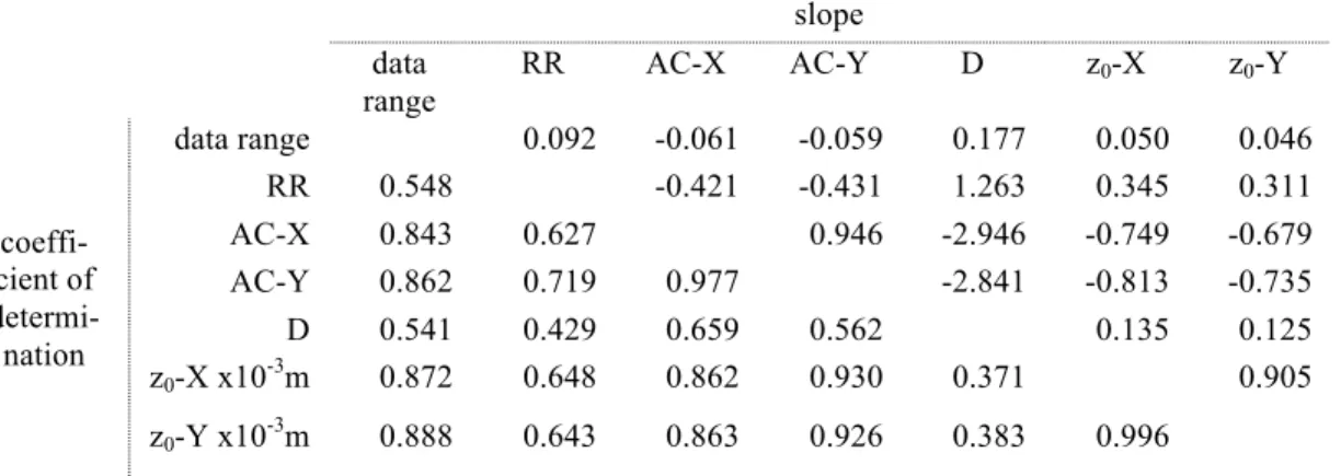
From the 12 datasets, geometric roughness is most correlated with the extreme surface elevations (data range) in a positive manner, and autocorrelation in a negative manner (Ta-ble 2). As expected the data range and autocorrelation are also well correlated. The fractal dimension is related to z0 (coefficient of determination, r2, values of 0.37), but mostly due
to the random nature of the NN surfaces.
Table 2. Comparison of the coefficient of determination and slope between data range, roughness metrics
and z0 based on the 12 interpolated datasets. The roughness metrics computed are the random roughness
(RR), average autocorrelation (AC) in both the X and Y directions, and the omni-directional fractal dimen-sion (D). The geometric roughness length (z0) was computed using the Lettau method in the X and Y
direc-tions. Units are the same as in Table 1.
slope data range RR AC-X AC-Y D z0-X z0-Y coeffi-cient of determi-nation data range 0.092 -0.061 -0.059 0.177 0.050 0.046 RR 0.548 -0.421 -0.431 1.263 0.345 0.311 AC-X 0.843 0.627 0.946 -2.946 -0.749 -0.679 AC-Y 0.862 0.719 0.977 -2.841 -0.813 -0.735 D 0.541 0.429 0.659 0.562 0.135 0.125 z0-X x10-3m 0.872 0.648 0.862 0.930 0.371 0.905 z0-Y x10-3m 0.888 0.643 0.863 0.926 0.383 0.996
5. Discussion and Conclusions
The distribution of snow depth (and at times snow water equivalent) has been performed over small areas (e.g., watersheds that are several km2 in size) using various techniques (e.g., Erxleben et al., 2002) such as binary regression trees and some of the methods used here. However, snowpack surfaces have rarely been interpolated, and spatial variation over space is typically over larger domains and at a coarser resolution. The focus of this work is not to compare the methods of interpolation for a snow surface but rather to capi-talize on the difference in the methods to yield varying surfaces in order to compare roughness metrics with geometric z0.
There can be an order of magnitude difference in the geometric z0 due in part to the
limitations of the Lettau [1969] method. The Lettau method “works well when roughness
elements are fairly isolated” [Businger, 1975]. When the cross-sectional area of a
rough-ness element becomes similar to the horizontal area of the element, z0 tends to be
overes-timated. When examining the interpolated snow surfaces, the different methods do not in-crease the average height of the elements, but do inin-crease the surface area (Figure 1). Alt-hough not shown graphically herein, the resolution of the data can be seen to influence the nature of the roughness elements produced using the IDW and NN methods. When more data are used, the existence of the elements is dampened due to the continuity of the sur-face from the raw data. This lowers the frontal area compared to using the 10-m subset da-ta; for the latter dataset individual obstacles stand out more yielding a larger z0.
There was some correlation between the patterns for geometric z0 estimation and the
dis-advantage over aerodynamic methods that most are based on empirical relations derived from wind tunnel work that deploys idealized flows over simplified arrays of roughness el-ements. In these simulations the flow is often relatively constant in direction, typically normal to the face of the elements, and the array is often regularly spaced (in rows or a staggered grid). These conditions differ significantly from those in nature, where wind di-rection is ever changing, and even if the topography is relatively regular, the size and shape of individual roughness elements (e.g. boulders and trees) are seldom regular.
Our study also allows the testing of the reliability of using microtopographic or surface elevation to compute z0, independent of wind profile measurements. However, concurrent
anemometric computations of z0 over snow should be compared with surface geometry,
i.e., roughness metrics and geometric z0. This should be performed for a wide range of
snow surfaces, such as those listed in the introduction (e.g., sastrugi, sun cups, melt rills). Other geometric methods exist to compute z0, such as Counihan [1971] and Macdon-ald et al. [1998]. These methods should be also evaluated, as well as the sensitivity of the different parameters in each formulation. Andreas [2011] refined an algorithm to relate the anemometric z0 to a physical roughness of the surface (ξ). The value of ξ was computed as
the integration of wave-number spectrum of the elevation of the snow-covered sea ice sur-face from wavelengths of 0.5 to 12.6 meters computed only in the upwind direction to a distance of at least 256 meters. When all wavelengths are used, i.e., integration from zero to infinity, ξ approaches the RR [Andreas, 2011]. It is suggested that future evaluation of geometric roughness extend to a similar distance using data at a resolution finer than 1 me-ter. Current light detection and ranging (lidar) technology will allow for such data to be collected.
Acknowledgements. Partial support was provided by the National Science Foundation through a Colorado State University (CSU) Center for Interdisciplinary Mathematics and Statistics (CIMS) grant, as well as a grant from the Colorado Water Center at CSU.
References
Andreas, E.L, 2011: A relationship between the aerodynamic and physical roughness of winter sea ice.
Quar-terly Journal of the Royal Meteorlogical Society, 137, 1581-1588.
Brock, B.W., I.C. Willis, and M.J. Sharp, 2006: Measurement and parameterization of aerodynamic rough-ness length variations at Haut Glacier d’Arolla, Switzerland. J. Glaciol., 52(177), 281-298.
Businger, J.A., 1975: Aerodynamics of vegetated surfaces. In Heat and Mass Transfer in the Biosphere: Part
1. Heat Transfer in the Plant Environment, (eds. D.A. de Vries and N.H. Afgan), pp. 139– 165, Scripta
Book Co., Washington, D.C.
Cline, D., S. Yueh, B. Chapman, B. Stankov, A. Gasiewski, D. Masters, K. Elder, R. Kelly, T.h. Painter, S. Miller, S. Katzberg, and L. Mahrt, 2009: NASA Cold Land Processes Experiment (CLPX 2002/03): Air-borne Remote Sensing. Journal of Hydrometeorology, 10(1), 338-346.
Counihan, J., 1971: Wind Tunnel Determination of the Roughness Length as a Function of the Fetch and Roughness Density of Three Dimensional Roughness Elements. Atmospheric Environment, 5, 637-642. Dong, W.P., P.J. Sullivan, and K.J. Stout, 1992: Comprehensive study of parameters for characterising
three-dimensional surface topography I: Some inherent properties of parameter variation. Wear, 159(2), 161-171.
Dong, W.P., P.J. Sullivan, and K.J. Stout, 1993: Comprehensive study of parameters for characterising three-dimensional surface topography II: Statistical properties of parameter variation. Wear, 167(1), 9-21. Dong, W.P., P.J. Sullivan, and K.J. Stout, 1994a: Comprehensive study of parameters for characterising
three-dimensional surface topography: III: Parameters for characterising amplitude and some functional properties. Wear, 178(1-2), 29-43.
three-dimensional surface topography: IV: Parameters for characterising spatial and hybrid properties.
Wear, 178(1-2), 43-60.
Davison, B.J., 2004: Snow Accumulation in a distributed Hydrological Model. Unpublished M.A.Sc. thesis, Civil Engineering, University of Waterloo, Canada, 108pp + appendices.
Deems, J.S., S.R. Fassnacht, and K.J. Elder, 2006: Fractal distribution of snow depth from LiDAR data.
Journal of Hydrometeorology, 7(2), 285-297.
Delaunay, B., 1934: Sur la sphère vide. Izvestia Akademii Nauk SSSR, Otdelenie Matematicheskikh i
Estestvennykh Nauk, 7, 793-800.
Elder, K. and A. Goodbody, 2004: CLPX-Ground: ISA Main Meteorological Data - Fraser Alpine ISA. NASA DAAC at the National Snow and Ice Data Center, Boulder, Colorado USA.
Elder, K., J. Dozier, and J. Michaelsen, 1991: Snow accumulation and distribution in an alpine watershed.
Water Resources Research, 27(7), 1541-1552.
Elder, K., D. Cline, A. Goodbody, P. Houser, G.E. Liston, L. Mahrt, and N. Rutter, 2009: NASA Cold Land Processes Experiment (CLPX 2002/03): Ground-Based and Near-Surface Meteorological Observations.
Journal of Hydrometeorology, 10(1), 330-337.
Erxleben, J., K. Elder, and R. Davis, 2002: Comparison of spatial interpolation methods for estimating snow distribution in the Colorado Rocky Mountains. Hydrological Processes, 16(18), 3627–364.
Fassnacht, S.R., 2010: Temporal changes in small scale snowpack surface roughness length for sublimation estimates in hydrological modeling. J. Geographical Research, 36(1), 43-57.
Fassnacht, S.R., M.W. Williams, and M.V. Corrao, 2009a: Changes in the surface roughness of snow from millimetre to metre scales. Ecol. Complex., 6(3), 221-229.
Fassnacht, S.R., J.D. Stednick, J.S. Deems, and M.V. Corrao, 2009b: Metrics for assessing snow surface roughness from digital imagery. Water Resources Research, 45, W00D31.
Foken, T., 2008: Micrometeorology. Springer Verlag.
Grimmond, C.S.B., and T.R. Oke, 1999: Aerodynamic properties of urban areas derived from analysis of sur-face form. J. Appl. Meteor., 38, 1262-1292.
Herzfeld,U.C, M. Helmut, N. Caine, M. Losleben, and T. Erbrecht, 2003: Morphogenesis of typical winter and summer snow surface patterns in a continental alpine environment. Hydrol. Processes, 17, 619-649 Holland, D.E., J.A. Berglund, J.P. Spruce, and R.D. McKellip, 2008: Derivation of effective aerodynamic
surface roughness in urban areas from airborne lidar terrain data. J. Appl. Meteor. Clim., 47, 2614-2625. Isaaks, E.H., and R.M. Srivastava, 1989: An Introduction to Applied Geostatistics. Oxford University Press,
New York.
Lettau, H., 1969: Note on Aerodynamic Parameter Estimation on the Basis of Roughness-Element Description. Journal of Applied Meteorology, 8, 828-832.
López Moreno, J.I. and D. Nogués Bravo, 2006: Interpolating snow depth data: a comparison of methods.
Hydrological Processes, 20(10), 2217-232 [doi:10.1002/hyp.6199].
Macdonald, R.W., R.F. Griffiths and D.J. Hall, 1998: An improved method for the estimation of surface roughness of obstacle arrays. Atmos. Environ., 32, 1857-1864.
Manninen, T., K. Antilla, T. Karjalainen and P. Lahtinen, 2012: Instruments and Methods - Automatic snow surface roughness estimation using digital photos. Journal of Glaciology, 58, 211, [doi:
10.3189/2012JoG11J144]
Miller, S. 2004: CLPX-Airborne: Infrared Orthophotography and Lidar Topographic Mapping - Fraser
Al-pine ISA. NASA DAAC at the National Snow and Ice Data Center, Boulder, Colorado USA.
Munro, D. S., 1989: Surface roughness and bulk heat transfer on a glacier: Comparison with eddy correla-tion. J. Glaciol., 35, 343-348.