Lessons learnt from the first EMEP intensive measurement periods

www.atmos-chem-phys.net/12/8073/2012/ doi:10.5194/acp-12-8073-2012

© Author(s) 2012. CC Attribution 3.0 License.

Chemistry

and Physics

Lessons learnt from the first EMEP intensive measurement periods

1_{Norwegian Institute for Air Research (NILU), Box 100, 2027 Kjeller, Norway} 2_{Norwegian Meteorological Institute, Oslo, Norway}

3_{Umweltbundesamt, Langen, Germany}

4_{Dept. Chemistry, Univ. of Gothenburg, Gothenburg, Sweden}

5_{Swedish Meteorological and Hydrological Institute, Norrk¨oping, Sweden}

6_{School of Physics & Center for Climate and Air Pollution Studies, Ryan Institute, National University of Ireland Galway,}

Galway, Ireland

7_{National Environmental Research Institute (NERI), Roskilde, Denmark} 8_{Umweltbundesamt, Vienna, Austria}

9_{Air Pollution, Environmental Technology EMPA, D¨ubendorf, Switzerland} 10_{Finnish Meteorological Institute (FMI), Helsinki, Finland}

11_{Centre for Ecology and Hydrology (CEH), Edinburgh, UK} 12_{Energy Centre of the Netherlands (ECN), Petten, The Netherlands}

13_{Institute of Environmental Assessment and Water Research (IDAEA-CSIC), Barcelona, Spain} 14_{CNR, The Institute for Atmospheric Pollution, Rome, Italy}

15_{Paul Scherrer Institut (PSI), Villigen, Switzerland}

16_{European Commission – DG Joint Research Centre, Ispra, Italy} 17_{Chalmers University of Technology, Gothenburg, Sweden}

18_{Leibniz Institute for Tropospheric Research (IfT) Leipzig, Germany} 19_{The Czech Hydrometeorological Institute (CHMI), Prague, Czech Republic} Correspondence to: W. Aas (waa@nilu.no)

Received: 9 January 2012 – Published in Atmos. Chem. Phys. Discuss.: 2 February 2012 Revised: 17 July 2012 – Accepted: 21 August 2012 – Published: 10 September 2012

Abstract. The first EMEP intensive measurement periods were held in June 2006 and January 2007. The measurements aimed to characterize the aerosol chemical compositions, in-cluding the gas/aerosol partitioning of inorganic compounds. The measurement program during these periods included daily or hourly measurements of the secondary inorganic components, with additional measurements of elemental-and organic carbon (EC elemental-and OC) elemental-and mineral dust in PM1,

PM2.5 and PM10. These measurements have provided

ex-tended knowledge regarding the composition of particulate matter and the temporal and spatial variability of PM, as well as an extended database for the assessment of chemi-cal transport models. This paper summarise the first experi-ences of making use of measurements from the first EMEP

intensive measurement periods along with EMEP model re-sults from the updated model version to characterise aerosol composition. We investigated how the PM chemical compo-sition varies between the summer and the winter month and geographically.

The observation and model data are in general agreement regarding the main features of PM10and PM2.5composition

and the relative contribution of different components, though the EMEP model tends to give slightly lower estimates of PM10and PM2.5 compared to measurements. The intensive

measurement data has identified areas where improvements are needed. Hourly concurrent measurements of gaseous and particulate components for the first time facilitated testing of modelled diurnal variability of the gas/aerosol partitioning of

8074 W. Aas et al.: Lessons learnt from the first EMEP intensive measurement periods nitrogen species. In general, the modelled diurnal cycles of

nitrate and ammonium aerosols are in fair agreement with the measurements, but the diurnal variability of ammonia is not well captured. The largest differences between model and observations of aerosol mass are seen in Italy during winter, which to a large extent may be explained by an underestima-tion of residential wood burning sources. It should be noted that both primary and secondary OC has been included in the calculations for the first time, showing promising results. Mineral dust is important, especially in southern Europe, and the model seems to capture the dust episodes well. The lack of measurements of mineral dust hampers the possibility for model evaluation for this highly uncertain PM component.

There are also lessons learnt regarding improved measure-ments for future intensive periods. There is a need for in-creased comparability between the measurements at differ-ent sites. For the nitrogen compounds it is clear that more measurements using artefact free methods based on continu-ous measurement methods and/or denuders are needed. For EC/OC, a reference methodology (both in field and labora-tory) was lacking during these periods giving problems with comparability, though measurement protocols have recently been established and these should be followed by the Par-ties to the EMEP Protocol. For measurements with no de-fined protocols, it might be a good solution to use centralised laboratories to ensure comparability across the network. To cope with the introduction of these new measurements, new reporting guidelines have been developed to ensure that all proper information about the methodologies and data quality is given.

1 Introduction

The “Cooperative programme for monitoring and evalua-tion of long-range transmission of air pollutants in Europe” (EMEP) was launched in 1977, and since 1979 EMEP has been an integral component of the Convention on Long-range Transboundary Air Pollution (LTRAP). The programme has continuously been evolving as new environmental topics and priorities in air pollution control policies have entered the arena (Tørseth et al., 2012). This creates new challenges on the monitoring programme, both for the number of param-eters to be monitored and for an increased density of sites. The growing demand for advanced monitoring, not least for obtaining new data for the EMEP model and other chemi-cal transport models evaluation, is however, difficult to meet for the Parties to the EMEP Protocol, especially since these increased needs are not necessarily coupled to correspond-ing increase in national fundcorrespond-ing. Furthermore, to facilitate data comparability across the network, it is recommended to establish standard or reference methods for the new parame-ters and/or measurement methods. In an intermediate phase, before full implementation of the continuous extended

mon-itoring program, shorter intensive measurement periods are a good compromise to generate datasets for model evalua-tion with acceptable geographical coverage. EMEP has pre-viously arranged a number of campaigns to provide data for parameters for which the monitoring technology is too ex-pensive or demanding to be a part of the regular programme, e.g. pilot measurements of nitrogen containing species in air in 1993–1994 (Semb et al., 1998) and the EC/OC paign during 2002–2003 (Yttri et al., 2007). These cam-paigns provide useful insight to atmospheric composition and processes, and are a necessary complement to the contin-uous measurements. Thus in the EMEP Monitoring Strategy for 2004–2009 (UNECE, 2004), campaign measurements, defined as intensive measurements periods (IMPs) were in-cluded as a part of the EMEP monitoring programme. IMPs are also incorporated in the strategy for the present period (2010–2019) (UNECE, 2009).

In the EMEP Monitoring Strategy it is stated that full chemical speciation of particles and gas/particle distribution should be conducted at EMEP super sites (Level-2 sites) whereas more advanced measurements (Level-3) with vari-ous research focus could be carried out in shorter periods. To assist the implementation of the monitoring strategy, the EMEP Task Force on Measurements and Modelling (TFMM) recommended conducting co-ordinated intensive measure-ments between the Level-2 sites, and the first two sam-pling periods were set for June 2006 and January 2007 (UN-ECE, 2005). Furthermore, additional research groups were involved with more advanced research activities (Level 3 measurements) at the same sites, i.e. with continuous mea-surements using aerosol mass spectrometer (AMS) or wet-chemistry techniques.

There were two main objectives for these first IMPs: (1) aerosol chemical speciation measurements to obtain a full mass closure for PM in several size fractions and (2) uti-lizing continuous online measurements to obtain high res-olution, size-resolved and near artefact free measurements of gas/aerosol partitioning of inorganic species. An important motivation for these intensive measurement periods was to obtain new insight in the spatial and temporal variation in PM chemical composition in order to facilitate further de-velopment of the EMEP model as well as other chemical transport models used in Europe. The measurements pro-vided data on mass closure of both coarse and fine particles (i.e. in PM10, PM2.5and PM1), and this information can help

explaining the existing discrepancies between modelled and observed mass of PM10 and PM2.5. Furthermore,

measure-ments of gas/aerosol partitioning, in particular for nitrogen species, and its diurnal variation pattern are essential for im-provement of our process understanding and its description in chemical transport models.

In this paper, we summarise the first experiences of mak-ing use of measurements from the first IMPs (June 2006 and January 2007), along with model results from the EMEP/MSC-W chemical transport model (Simpson et al.,

Table 1. Measurements being conducted during the EMEP intensive periods in June 2006 and January 2007.

Sites Mass Daily Hourly

Inorg. EC/OC Dust Inorg EC/OC

Jun 06 Jan 07 Jun Jan Jun Jan Jun Jan Jun Jan Jun Jan

AT02 Illmitz PM10, PM2.5, PM1 PM10, PM2.5, PM1 FP FP SO4 PM2.5

CH02 Payerne PM10, PM2.5, PM1 PM10, PM2.5, PM1 X X AMS AMS PM2.5 PM2.5

CZ03 Koˇsetice PM10, PM2.5 PM10, PM2.5 PM10 PM10

DE02 Langenbr¨ugge PM10, PM2.5, PM1 PM10, PM2.5, PM1 FP

DE03 Schauinsland PM10, PM2.5 PM10, PM2.5 FP

DE07 Neuglobsow PM10, PM2.5 PM10, PM2.5 FP

DE44 Melpitz PM10, PM2.5, PM1 X X X X AMS AMS

DK41 Lille Valby PM10, PM2.5, PM1 PM10, PM2.5, PM1 ES1778 Montseny PM10, PM2.5, PM1 PM10, PM2.5, PM1 X X X X X X FI17 Virolahti II PM10, PM2.5, PM1 PM10, PM2.5, PM1 X X GB33 Bush AMS GB36 Harwell PM10, PM2.5 IC PM10 GB48 Auch. Moss IC IC

IE31 Mace Head PM2.5 AMS AMS

IT01 Montelibretti PM10, PM2.5 PM10, PM2.5 X X X X X X

IT04 Ispra PM10, PM2.5 PM10, PM2.5 PM2.5 PM2.5 PM2.5 PM2.5 IC IC

NL11 Cabauw PM10, PM2.5 PM10, PM2.5 IC IC

NO01 Birkenes PM10, PM2.5, PM1 PM10, PM2.5, PM1 X X X X

FP: Filterpack; X:. Speciation in two or three sizes size fractions; AMS: Aerodyne Mass Spectrometer; IC: SJAC/MARGA/GREAGEOR (water soluble inorganic ions); OM: Organic mass.

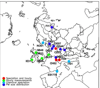
FI17 GB48 GB33 NO01 IE31 GB36 ES1778 IT01 IT04 CH02 DE03 NL11 DK41 DE07 DE02 DE44 CZ03 AT02

Fig. 1. Sites that took part in the EMEP intensive measurement pe-riods in June 2006 and/or January 2007.

2012, here we use version rv4β), to characterise aerosol com-position. We investigated how the PM chemical composition varies between the summer and the winter month and ge-ographically. The main results of comparison of intensive measurements with model calculations are presented and dis-cussed, along with the consideration of encountered prob-lems and data inconsistencies.

2 Methodology

2.1 Measurement programme, sites and methods The first EMEP IMPs lasted from 1 to 30 of June 2006 and from 8 of January to 4 of February 2007. The measurement programme at the various sites is described in Table 1, and the locations of the sites are shown in Fig. 1. Several sites measured aerosol mass concentrations in three size fractions, PM1, PM2.5, and PM10, though not all of them provided the

full chemical speciation. Only data from sites with PM chem-ical composition including at least both secondary inorganic aerosols and carbonaceous matter are selected for compari-son with the EMEP model results for chemical composition. In addition, some of the continuous measurements are used to evaluate model calculated diurnal variation of gaseous and aerosol nitrogen compounds. For a more comprehensive analysis of the hourly data, the reader is referred to Nemitz et al. (2012). The measurements are compared with the av-erage concentrations predicted by the EMEP model for the model grid cell, within which the site is located. Although EMEP measurement sites are selected to represent the rural regional background, it is recognised that in some cases the site is not always representative for the whole grid cell, i.e. IT04 which is situated close to the south eastern border of the cell, is more influenced by regional pollution from the Po valley compared to the grid cell on average.

All the data reported from these intensive periods are available from the EMEP data base (http://ebas.nilu.no). An overview of the methods used for chemical composition mea-surements is provided in Table 2. The methods, as well as some known artefacts and data inconsistencies are briefly de-scribed below.

8076 W. Aas et al.: Lessons learnt from the first EMEP intensive measurement periods

Table 2. Methods in field and laboratory for sites with chemical composition of daily measurements (manual method) in PM₁₀and PM_2.5 of inorganic and organic components.

Site Field methods Analytical method

Sampler Mass Inorganic EC/OC Mineral dust

CH02 Digitel DHA80. Quartz

filters (QMA).

Gravimetric, EN 12341

IC (from quartz filters)

Sunset Monitor, denuder, TOA//NIOSH 5040

DE44 Digitel DHA80. Quartz

filters (MK360). Filter face velocity: 54 cm s−1 Gravimetric EN 12341 IC (from quartz filters) VDI 2465 -part 2

ES1778 Digitel DHA80 Quartz

filters (Schleicher and Schuell, QF20). Simul-taneously PM₁₀, PM_2.5 and PM1mass

concen-tration continuously

with optical particle

counters, corrected

with factors obtained by the gravimetric data.

Gravimetric, EN 12341 IC and ammo-nium selective electrode (from quartz filters) Sunset analyzer TOT technique, NIOSH protocol ICP-AES and ICP-MS from total acidic digestion of quartz filters

IT01 Tandem quartz filter

(QBQ) Filter face velocity: 54 cm s−1 beta attenuation method (OPSIS SM200) IC (from Teflon filters and de-nuders)

Sunset TOA NIOSH

5040.Corrected for

positive artefact in June

ED-XRF (Teflon filters) IT04 Single quartz filter,

de-nuder. Filter face veloc-ity: 24 cm s−1

Gravimetric, quartz filter, not conditioned

IC (from quartz filters)

Sunset .TOA, EUSAAR-1. Corrected for positive artefacts

NO01 Tandem quartz filter

(QBQ). Filter face

velocity: 54 cm s−1

Gravimetric, quartz filter, not conditioned

IC (from quartz filters)

Sunset. TOT, EUSAAR-1. Corrected for positive artefact in June

2.1.1 Aerosol mass

The reference method for mass measurements based on gravimetry in accordance to EN 12341 (CEN, 1999) were used at most sites, though there were some exceptions. IT01 used the beta attenuation monitor (OPSIS SM200) and PM2.5

is measured with a tapered element oscillating microbalance (TEOM) at DK41. At GB36, PM10 and PM2.5 were

mea-sured with TEOM in parallel with PM2.5 gravimetric

mea-surements. The gravimetric data are substantially higher than the TEOM measurements at this site, i.e. PM2.5in June 2006

is 13.5 µg m−3and 23.5 µg m−3for TEOM and the gravimet-ric method, respectively. The TEOM instruments had a tem-perature of 50oC and it is expected a loss of volatile com-pounds. The difference is therefore probably partly due to the inherent problems of measuring semi-volatile aerosols with the TEOM and problems to define an appropriate correction factor (e.g. Hauck et al., 2004). For comparability between fine and coarse fraction, the TEOM data from GB36 have however been used, though as shown above, these should be considered as lower estimates. For ES1778 PM10, PM2.5

and PM1mass concentrations were derived from continuous

measurements with an optical particle counter (OPC, Grimm dust monitor 1107) using conversion factors obtained from

simultaneous gravimetric analyses. PM10 and PM2.5 filter

sampling was performed for gravimetric and chemical anal-ysis at a rate of two filters per week. Quality assurance is a challenge with mass measurements because the required val-idation in accordance to EN12341 (CEN, 1999) of alternative measurements to the reference method is often done in urban areas and thus not necessarily representative for the EMEP sites. Furthermore, regular laboratory intercomparison of the weighing procedures has not yet been established. Work is in progress to better assess the quality of the mass measure-ments in EMEP.

2.1.2 Water soluble inorganic ions

The daily aerosol chemical speciation measurements were performed through water extraction of the aerosol filters and analysis by ion chromatography, except at ES1778 where NH+₄ was analysed with a selective electrode, Table 2. The filters were either of Teflon®or quartz using the regular fil-terpack measurements with no size cut-off and/or the wa-ter extracts from the gravimetric measurements of PM10

and PM2.5. These measurements are typically biased with

possible evaporation of ammonium nitrate aerosol (negative artefact) and potential absorption of gaseous nitric acid and

ammonia on the aerosol filter (positive artefact). The only exception is IT01, which used the reference denuder/filter method where one would expect only little, if any, bias in the gas/particle separation. For the filterpack method, the evapo-ration of NH4NO3from the aerosol front filter will lead to the

capture of additional HNO3and NH3on the impregnated

fil-ters and an overestimation of the gas-to-aerosol ratio, while capture of NH3 and HNO3 on the front aerosol filter will

give an underestimated ratio. The sum of nitrate and sum of ammonium in the filter pack measurements are unbiased (EMEP, 2001)

The hourly inorganic measurements were either performed using an aerosol mass spectrometer (AMS) (Jayne et al., 2000; DeCarlo et al., 2006) or wet-chemistry techniques. These couple sequential sampling with a wet annular de-nuder (WAD) and steam jet aerosol collector (SJAC) to on-line ion chromatograph (IC), here deployed in three differ-ent incarnations (MARGA, GRAEGOR, WAD-SJAC; see Thomas et al., 2009). The wet chemistry techniques mea-sure both gaseous and particulate species with a specific cut-off size (PM10 and/or PM2.5). The cut-off of the AMS is

characterised by 100 % transmission for 70-600 nm particles and some transmission up to beyond 1 µm and down to 30 nm. Thus, the size of measured NH4NO3, (NH4)2SO4 and

NH4Cl aerosols approximately corresponds to PM1. While

the wet-chemistry instruments detect any water soluble com-ponents (much like the filter extractions), the AMS detects only aerosol components that volatilise at 600◦C, i.e. usu-ally KCl, K2SO4, NaCl, NaNO3and Ca2NO3in PM1are not

detected.

Some of the components, which were measured in parallel with different methodologies, gave inconsistent results. At CH02, PM1 chemical speciation was determined from

par-allel filters and continuous AMS measurements. The differ-ence was especially large for NO−₃, which hardly could be detected from the PM1filters during June 2002 (Fig. 2). In

January 2007, the difference was 40 %, similar as for am-monium. The ammonium concentrations from filter samples were 30 % lower compared with the AMS data in summer. Sulphate were similar for the two type of measurements, somewhat underestimated by the AMS in June possibly due to not detectable sulphate species (i.e. CaSO4) or small

dif-ferences in the transmission curves of the inlets. For mass closure of PM2.5at CH02 in this work, we combine the

inor-ganic components in PM1 from filter (SO2−₄ , sea salts) and

AMS (NH4 and NO3), and the carbonaceous matter

mea-sured in PM2.5using monitor. It is expected that most of the

fine particle secondary inorganic aerosols (SIA) resided in the PM1fraction resemble what is expected in PM2.5.

At NO01 the data is considered unreliable for the SIA components in both size fractions in January 2007. The con-centration levels were very low, especially for nitrate and am-monium, dropping below the detection limit of the IC anal-ysis in many days. The regular filterpack data (with no size cut) from the same period seems more reasonable, and we

0 1 2 3 4 5 6 SO4 NO3 NH4 Ae ros ol Mass ( m g/ m 3) summer AMS summer PM1 gravimetric winter AMS winter PM1 gravimetric

Fig. 2. Comparison of chemical speciation measurements using AMS and filters from gravimetric PM1sampler at Payerne, CH02.

have therefore used these as a proxy for the nitrate and am-monium in PM10.

2.1.3 Carbonaceous matter

Measurement of elemental carbon (EC), organic carbon (OC) and total carbon (TC) in PM10and PM2.5were conducted at

six sites. The quartz fibre filters used were preheated for 3 h at 900◦C to minimize blank values of OC. Various protocols were applied for analysis (Table 2), thus hampering the com-parability of these data.

Although the analytical approaches vary, it is generally accepted that the total carbon (TC) should be comparable. Putaud et al. (2010) estimates that the discrepancies of TC across the European measurements is smaller than ± 25 % whilst the split between EC and OC is more site specific de-pending on methodology. The thermal optical analysis cor-rects for charring of OC during analysis, however different temperature programs are used (i.e. EUSAAR 1 and NIOSH (Table 2), which impact the split between EC/OC. Further, the VDI 2449 method provides TC levels comparable to the thermal optical methods, but overestimates EC as it does not account for charring of OC (Schmid et al., 2001; Cavalli and Putaud, 2011).

The collection of filter samples for subsequent analysis of OC is associated with positive and negative sampling artefacts. IT01 and NO01 used tandem filter set-ups (Mc-Dow and Huntzicker, 1990) operating according to the QBQ-approach (quartz-fibre filter behind quartz fibre filter) to ac-count for the positive artefact of OC. The positive artefact of OC at these two sites accounts for 30–50 % of OC in June. The backup filter was not analysed in January at either of these sites, in Norway, due to very low level of OC. Thus the OC data at IT01, NO01 in January 2007 were not corrected for positive artefacts. IT04 and CH02 used a denuder to re-move the gaseous organic compounds before they reach the filter. Neither of those four sites, which used denuders or the

8078 W. Aas et al.: Lessons learnt from the first EMEP intensive measurement periods QBQ-approach, accounted for negative artefacts, thus they

provided a low estimate of OC.

For chemical mass closure of PM10and PM2.5the amount

of organic matter mass (OM) is usually calculated applying a conversion factor to OC to account for non-C components. However, in this paper we have chosen not to apply any con-version factor for OC nor EC, since the concon-version factor may vary considerably between the sites (Yttri et al., 2007; Putaud et al., 2010), adding uncertainties to the comparison between model and measurements. The non-carbonaceous OM is included in what is defined as “other”, and compari-son with model focuses on the OC component only. The car-bonaceous fraction in the PM composition should therefore be considered generally underestimated.

2.1.4 Mineral dust

The measurements of mineral compounds were performed using XRF at IT01 and ICP-AES and ICP-MS from solu-tions obtained by total acidic digestion of the filter at ES1778 (Pey et al., 2010). Mineral dust mass (DU) was derived from measurement data, using the formula suggested by Chan et al. (1997):

DU = (1.89 · Al + 2.14 · Si + 1.4 · Ca + 1.2 · K + 1.36 · Fe) · 1.12(1) where all concentrations are in µg m−3. For the other sites, water soluble calcium may be used as an indicator of min-eral dust; however, that has not been applied here for the model measurement intercomparison since the model does not calculate the individual mineral components. Neverthe-less, modelled dust is included in the chemical speciation calculations even at sites with no dust measurements. 2.2 Model description

The EMEP MSC-W chemical transport model, version rv4β, has been used for the calculations. The full description of the model is given in Simpson et al. (2012) (for version rv4, we will note differences where relevant). The model calcu-lation domain covers the whole of Europe, and includes a large part of the North-Atlantic and the Arctic areas. The model resolves 20 vertical layers, reaching a height of 100 hPa. The lowest model layer is approximately 90 m thick. In the present calculations, the horizontal resolution of approx-imately 50×50 km2was used.

The EMEP model describes the emissions, chemical trans-formations, transport and dry and wet removal of gaseous and particulate air pollutants. The basic EMEP photo-oxidant and inorganic aerosol scheme uses about 140 reactions be-tween 70 species (Andersson-Sk¨old and Simpson, 1999; Hayman et al., 2012, Simpson et al., 2012), and in addition a scheme for secondary organic aerosol (SOA), derived from Bergstr¨om et al. (2012) has been implemented. In the model, SO2is oxidised to sulphate in the form of H2SO4in the gas

phase by OH and in the aqueous phase by H2O2 and O3.

In the daytime and in summer, NO2oxidation occurs mainly

through reaction with OH, while in the night time and in win-ter its oxidation is predominantly by ozone on deliquescent aerosols. An important source of nitrate in the troposphere is the reaction of N2O5on deliquescent aerosols, producing

HNO3, which further takes part in the formation of

ammo-nium nitrate and/or coarse nitrate on sea salt and dust par-ticles. Ammonium sulphate is formed instantaneously from NH3and H2SO4. The MARS equilibrium model (Binkowski

and Shankar, 1995) is used to calculate the partitioning of inorganic species (HNO3/NO−₃ and NH3/NH+₄) between the

gas and aerosol phase as a function of relative humidity and temperature. Coarse nitrate formation from HNO3 is

presently assumed to take place at a rate which depends on relative humidity.

The EMEP model combines the calculated aerosol chem-ical components treated by the model to predict the mass concentration of two size fractions for aerosols, fine aerosol (PM2.5) and coarse aerosol (PM10−2.5). The aerosol

com-ponents included in the model are sulphate (SO2−₄ ), nitrate (NO−₃), ammonium (NH+₄), anthropogenic elemental (EC) and organic aerosol (primary and secondary from both an-thropogenic and biogenic sources), sea salt and mineral dust (from anthropogenic sources and windblown).

Ammonium nitrate is assumed to be all associated with PM2.5. While all ammonium is assumed to be solely in the

fine fraction (as ammonium nitrate or ammonium sulphates), calculated coarse NO−₃ is assumed to be evenly split between PM2.5 and PM10−2.5 so that half of the coarse NO−3 mass

is attributed to each size fraction. In the model, coarse ni-trate represents nini-trate aerosol formed on sea salt and min-eral dust. When comparing calculated PM2.5 with

observa-tions, the model accounts that a portion of the nitrate associ-ated with sea salt and dust resides on aerosols with diameters smaller than 2.5 µm, and thus contributes to PM2.5 mass. In

this rv4β model version, the Mass Median Diameter (MMD) of coarse nitrate is assumed to be 2.5 µm (whereas fine ni-trate has MMD of 0.33 um), and we assume that 50 % of this is in the fine (PM2.5). This treatment reflects an

assump-tion that most coarse nitrate is being formed on sea-salt, with condensation occurring at the lower end of the coarse parti-cle mode, which has highest surface-area (see e.g. Pakkanen et al., 1996, Simpson et al., 2012). On the other hand, coarse nitrate formed on dust particles may have MMD larger than sea salt associated nitrate (e.g. 3.8 µg as in data by Pakkanen et al., 1996). Thus, in the areas of large influence of mineral dust, the EMEP model will probably overestimate nitrate in PM2.5. This split between PM2.5and PM2.5−10for nitrate is

clearly rather uncertain, and currently work is in progress to implement an explicit formation of nitrate on sea salt and dust aerosols, which in principal should lead to a sounder process description. (In version rv4, a larger MMD of 3 µm was assumed for coarse nitrate, giving a lower fraction of coarse NO3in the PM2.5range).

Aerosol water is calculated as function of the ambient rel-ative humidity and temperature based on PM chemical com-position. For consistent comparison with observations, the model also estimates the water content in PM10 and PM2.5

gravimetric mass determined according to the EN 12341 standard (CEN, 1999), i.e. at 20◦C temperature and 50 % rel-ative humidity (Tsyro, 2005). Aerosol water is necessary to estimate the total mass, but in the model the water content calculated is not influencing the partitioning between fine and coarse particles, nor the deposition processes. Dry de-position parameterisations for aerosols are calculated as in Simpson et al. (2012), accounting for aerodynamic and lam-inar sub-layer resistances and also for gravitational settling of larger particles. Meteorology and land-use dependent dry deposition velocities are calculated for the different aerosol size fractions. Wet scavenging is treated with simple scav-enging ratios, taking into account in-cloud and below-cloud processes. The scavenging ratios for aerosols reflect the com-ponent’s solubility, and size differentiated collection efficien-cies are employed in below-cloud aerosol washout.

The model calculations presented in this work were performed using emission data from the EMEP emission database (http://www.ceip.at/emission-data-webdadab). The split of primary fine PM emissions to carbonaceous and inor-ganic mass, and the remaining primary component was made based on the estimates by Kupiainen and Klimont (2007) and Z. Klimont (personal communications, 2010).

Three-hourly meteorological fields from the ECMWF-IFS model (http://www.ecmwf.int/recearch/ifsdocs/) were used to drive the calculations of pollutant atmospheric transport.

3 Results and discussion

3.1 Aerosol mass and chemical composition

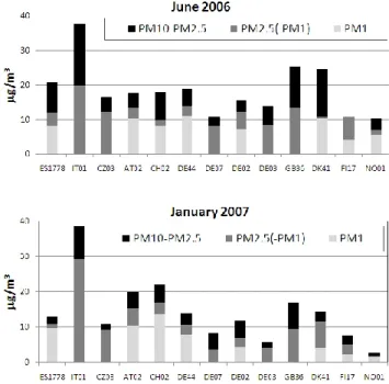
All the sites with mass measurements in two or three size fractions have been compared to assess the variations in size distribution, Fig. 3. For all size fractions, the lowest con-centrations of PM are seen in the Nordic countries and the highest in Italy. The aerosol mass was in general somewhat higher in June compared to January for all size fractions, ex-cept at AT02, CH02 and IT01, and at IT04 for PM2.5, where

the winter concentrations are somewhat higher. At the Ital-ian sites, the high PM concentrations in winter compared to summer are mainly attributed to the high carbonaceous aerosol loading in winter (chapter 3.1.2). At IT04 and CH02 also enhanced ammonium nitrate was observed in January 2007. Such differences were already documented by Lanz et al. (2007, 2008) for an urban background station in Switzer-land. It should be noted that the during winter the increase pollution episodes are often due to worse pollution disper-sion in winter, thus bad vertical mixing.

Measured PM10and PM2.5mass have been compared with

the EMEP model, and scattered plots are seen in Fig. 4. The

Fig. 3. Size distribution of the aerosol mass during the EMEP in-tensive measurement periods. Note that not all the sites have PM₁ measurements. PM2.5(PM1) is the difference between PM2.5 and PM1for those sites having both these measurement, otherwise it is representing the PM25fraction.

model calculated PM10and PM2.5concentrations are mostly

within 30 % of observed values. The model gives somewhat lower PM2.5and PM10mass compared to measurements, but

the bias is in general quite small (between 4 % and 19 %). The exception is PM2.5 in January 2007, where the model

estimates 34 % less than the measurements. The spatial dis-tribution of both PM2.5and PM10is better reproduced by the

model in June 2006 compared to January 2007 (as shown by correlation coefficients in Fig. 4), though different number of sites are included in the scatter-plots and statistics.

The fine/coarse ratio is quite similar for the two periods. On average PM1 and PM2.5 are about 50 % and 70 % of

PM10, respectively for both seasons. However, there are large

variations between the sites, PM1ranging from 30–75 % of

PM10 in winter (less spread in summer), while the PM2.5

fraction of PM10 range from about 40 % to almost 100 %

in both periods. Most sites have larger fractions of coarse particles in summer than winter probably due to bigger con-centrations of coarse particles like mineral dust and primary biological aerosols particles (PBAP) in summer (e.g. Yttri et al., 2011; Querol et al., 2009). The measurements presented here are limited in time and space, and thus it is difficult to draw general conclusions from them. For further details on the regional mass and chemical composition measurements, the reader is referred to the EMEP PM reports and ments (e.g. Tsyro et al., 2011a; EMEP, 2007) and the assess-ments of the European aerosol phenomenology by Putaud et al. (2004, 2010). In the regular EMEP data (Tsyro et al.,

8080 W. Aas et al.: Lessons learnt from the first EMEP intensive measurement periods Bias: -4% Corr.: 0.60 Bias: -2% Corr.: 0.61 Bias: -34% Corr.: 0.35 Bias: -35% Corr.: 0.36 Bias: -16% Corr.: 0.81 Bias: -16%

Corr.: 0.81 Bias: -18% _{Corr.: 0.37}

Fig. 4. Scattered plot of model and measured PM10 and PM2.5 mass during the EMEP intensive measurement periods.

2011a), the highest PM2.5/PM10is commonly seen for

cen-tral European sites, which are relatively more influenced by anthropogenic sources. In contrast, mineral dust in the south of Europe and PBAP in northern Europe contribute relatively more to the coarse fraction of PM10.

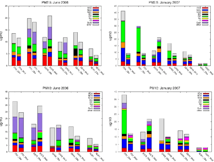
In order to explain the discrepancies between calculated and observed PM masses, we look closer at the individual aerosol components forming PM. The chemical composition of PM calculated with the EMEP model has been compared with PM mass closure data from the intensive periods for the sites reporting both inorganic and carbonaceous compo-nents, in total six sites. Figure 5 compares observed and cal-culated chemical composition of PM10and PM2.5, averaged

over each of the measurement periods, and displayed in four panels. Each panel shows a pairs of bar-diagrams for each of the sites: observations (left) and model results (right). The

heights of the bars correspond to the measured or calculated PM concentration.

The observation and model data are in general agreement regarding the main features of PM10and PM2.5composition

in different geographical locations and the relative contribu-tion of the individual aerosol components. The results are fairly consistent with respect to the specifics of PM compo-sition in the summer and winter month, and different size fractions. Organic carbon, together with sulphates in sum-mer and nitrate in winter, appear the most important PM constituents. Mineral dust becomes dominating in PM10 at

the southern sites in June 2006. It should be noted that there are fundamental limitations in how well the model (on a 50x50 km2grid) and measurements (from one point) can be expected to compare, due to the large temporal and spatial variability of atmospheric aerosols, their size distributions, chemical and physical properties, chemical formations and

Fig. 5. Observed and modelled chemical composition of PM10(bottom) and PM2.5(top) for June 2006 (left) and January 2007 (right), from observations and model results. “Other” denotes not determined PM mass in measurements, and particle water + missing carbonaceous matter (OM-OC) in calculations. Note: (1) Full mineral composition was measured only at IT01 and ES17, (2) Very few days (1–6) with data at ES1778, besides different coverage for different components; (3) measured PM2.5speciation at CH02 is based on daily SIA in PM1and hourly EC/OC in PM_2.5data; (4) measured nitrate and ammonium in PM₁₀at NO01 in January 2007 are from filterpack.

transformations, etc. More detail discussions of PM individ-ual components are given in the next sections.

As seen for all the sites with mass measurements dis-cussed above (Fig. 4), the model tends to predict lower con-centrations of PM10 and PM2.5 compared to measurements

for most of these sites except from Montseny (ES1778) for both June 2006 and January 2007 and Payerne (CH02) in June 2006 (Fig. 5 and Tables 3–4). Comparison of these re-sults with the PM scatter-plots in Fig. 4 reveals that the es-timated PM10 is lower by the model somewhat more for the

smaller selection of sites with chemical composition mea-surements (Table 3) compared to the average for a larger selection of sites (Fig. 4). Table 3 and Figure 5 show that the low model PM10 concentrations compared to

measure-ments are due to its underestimation of most of the individual

PM components, with the exception of nitrate and in some cases ammonium. At ES1778 (both periods), the model gives higher concentrations of all PM components compared to measurements, and consequently PM10 (Fig. 5). Regarding

the performance for PM2.5, the model gives lower estimates

of PM2.5 than measurements, and the difference is typically

larger for the winter month than for June 2006, Fig. 5. This is consistent with the general pattern shown in Fig. 4. The high-est differences for January 2007 are seen at the Italian sites, IT01 and IT04 (Figs. 4 and 5; Tables 3 and 4). One possible reason for this might be problems in resolving wintertime dispersion (e.g. very low mixing heights), but Bergstr¨om et al. (2012) and Denier van der Gon et al. (2012) con-cluded that there are also major uncertainties in the emission

8082 W. Aas et al.: Lessons learnt from the first EMEP intensive measurement periods

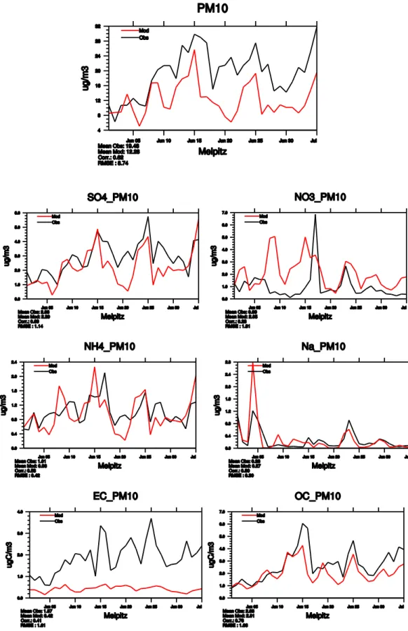
Fig. 6. Daily chemical speciation in PM10at Melpitz (DE44) in June 2006 from measurements (black) and EMEP model (red).

inventory, likely the biomass burning component, for winter emissions in the areas around these.

The quality of the model output is certainly very depen-dent on good emission data. The emission estimates may have different quality depending on region. The Melpitz site (DE44) typically experiences significant higher concentra-tion levels of PM10 and PM2.5 during easterly winds

com-pared to westerly (Spindler et al., 2010). In June 2006, about seven days at Melpitz were influenced from this type of

long-range transport and measurements show significantly higher particle mass concentrations compared with the other days. Chemical transport models have generally shown too low particle mass concentrations for long-range transport from eastern directions in Central Europe compared to measure-ments at DE44 (Renner and Wolke, 2006; Stern et al., 2008) indicating problems with the emissions from this region. When investigating the measurements from the EMEP IMP in more detail, one can see that the EMEP model captures the

Table 3. Comparison statistics between model calculations and observations for PM₁₀component. PM10 SO2−₄ NO−₃ NH+₄ EC OC Na+ Miner. IT01 2006 Bias -28 -45 42 -27 -61 -26 -58 22 R 0.92 0.73 0.7 0.81 0.3 0.41 0.72 0.9 2007 Bias −66 −58 −31 −49 −42 −88 −17 −81 R 0.59 0.46 0.34 0.4 0.55 0.59 0.58 0.61 DE44 2006 Bias −35 −28 101 −10 −76 −23 7 R 0.58 0.7 0.18 0.52 0.54 0.77 0.79 2007 Bias −11 9 −2 13 −53 −17 53 R 0.47 0.55 0.67 0.52 0.76 0.61 0.75 NO01 2006 Bias −42 −53 28 −42 8 4 −23 R 0.75 0.81 0.52 0.66 0.81 0.69 0.55 2007 Bias 18 25 −89∗ 0∗ 20 62 11 R 0.42 0.36 0.02∗ 0.06∗ 0.34 0.09 0.15 ES1778 2006 Bias 36 14 176 188 281 89 4 40 R 0.72 0.55 −0.45 0.77 −0.24 0.15 0.67 0.84 2007 Bias 76 21 174 290 147 9 R 0.85 0.70 0.83 0.54 0.51 0.22

Temporal data coverage: roman font cells – 90–100 % coverage, italic font cells – about 30–50 % coverage. ∗_{Filterpack measurements were used (see details in the text).}

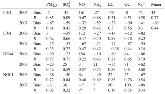
Table 4. Comparison statistics between model calculations and observations for PM2.5components

PM2.5 SO2−₄ NO−₃ NH+₄ EC OC Na+ Miner IT01 2006 Bias -7 -42 161 -27 -59 -8 -71 44 R 0.85 0.89 0.67 0.88 0.31 0.51 0.58 0.77 2007 Bias −67 −59 −32 −52 −32 −90 −41 −69 R 0.61 0.41 0.29 0.43 0.3 0.56 0.3 0.44 IT04 2006 Bias 3 −39 112 −27 −14 −12 −82 R 0.62 0.66 0.47 0.50 0.87 0.78 0.23 2007 Bias −75 −57 −67 −71 −77 −87 −55 R 0.25 0.22 0.47 0.42 −0.28 0.44 0.24 DE44 2006 Bias −29 −23 154 −10 −89 64 −60 R 0.57 0.71 0.22 0.43 0.27 0.65 0.79 2007 Bias −23 25 3 21 −35 71 −62 R 0.42 0.59 0.57 0.55 0.83 0.6 0.68 NO01 2006 Bias −38 −50 64 −45 22 25 −67 R 0.72 0.84 0.46 0.69 0.83 0.78 0.54 2007 Bias −3 36 −∗ ∗ 50 100 −89 R 0.02 0.32 -∗ ∗ 0.19 0.35 0.34

ES1778 not included due to low data capture, CH02 not included due to non concurrent measurements. ∗_{Data problems at NO01.}

SIA and sea salt components very well, except for one major nitrate episode on 17 June (Fig. 6). The major PM episodes (i.e. 15 June) have large contributions of carbonaceous mat-ter, which are captured by the model. The EC levels esti-mated by the model are much lower than the observed val-ues, although as noted in Sect. 2.1.3, the EC measurements at DE44 are overestimates, as they have not been corrected for charring of OC (Sect. 2.1.3; Schmid et al., 2001; Cavalli and Putaud, 2011). These examples also illustrate the impor-tance of daily or higher resolution measurements for studying sources and comparison with model.

3.1.1 Secondary inorganic aerosols (SIA)

The SIA concentrations increase from the northern European site (NO01) to the central (DE44) and southern (ES1778) Eu-ropean sites; with even higher values found at IT01 (semi-rural) and IT04 (polluted Po Valley). This is in accordance with observations from the regular EMEP network where the SIA contribute on average (from 17 sites) 34± 13 % to the PM10mass in 2009, with the highest contribution in central

Europe (Aas and Tsyro, 2011). SO2−₄ and NH+₄ seasonal vari-ation reflects enhanced photo-oxidvari-ation rates of sulphur and

8084 W. Aas et al.: Lessons learnt from the first EMEP intensive measurement periods greater abundance of ammonia in summer, whereas lower

temperatures and higher relative humidity favours formation of nitrate aerosol in winter. The relative contribution of SIA and the seasonal variations are comparable in the model and measurements.

Modelled sulphate concentrations in both PM10and PM2.5

tend to give 23 and 53 % lower than observations in summer at all sites (Tables 3 and 4). The situation changes in win-ter, when SO2−₄ is even more lower than observations (57-59 %) in the southern (Italian) sites, but higher than observa-tions by 9-36 % at the sites in central and northern Europe (DE44 and NO01). At the Spanish site ES1778, the model is slightly higher than observed SO2−₄ in PM10 both in June

2006 and January 2007, though too few days with PM2.5data

were available at this site. The results are in general similar for SO2−₄ in PM10and PM2.5, which is as expected since

sul-phate is mainly found in the fine fraction. However, larger un-derestimation and smaller overestimation by the model com-pared to measurements are found for SO2−₄ in PM10

com-pared to PM2.5at DE44 and NO01, as only fine SO2−4 is

cal-culated by the model. Those results are in line with compar-ison of model with standard EMEP observations, although the bias seen here is larger (Fagerli et al., 2011). The EMEP model generally represents sulphate better than e.g. the ni-trogen species when looking at a larger dataset than what is the case for the limited numbers in this study (Fagerli et al., 2011). However, the difference in performance between the different aerosol components (at least SO4, NO3, NH4)

is rather small, Tables 3 and 4. This can probably at least partly be attributed to uncertainties in modelling of dry and wet depositions of the aerosols, which is difficult for all of the species. Furthermore, although emission inventories of SO2 are well known, information of the temporal

distribu-tion (e.g. the summer to winter ratio) is not so well known. Model performance for SO2−₄ has recently been considerably improved due to improved description of cloud water acidity and also changed the temporal profile of SOxemissions.

Nitrate tends to be lower in the model compared to obser-vations, especially NO−₃ in PM2.5 in June 2006. The

excep-tions are IT01 and IT04 in January 2007, where the modelled NO−₃ in PM2.5 is 32 % and 67 % lower than observations,

respectively. These results are in general better than earlier model calculations, which considerably underestimated ni-trate (Fagerli et al., 2011). Recent improvements have been achieved by changing to the use of the MARS equilibrium model (Binkowski and Shankar, 1995) for ammonium nitrate formation, and by accounting for a part of coarse NO−₃ within PM2.5mass (Sect. 2.2). Reasons for the overestimation might

include incorrect size-distribution assumptions, uncertainties in the formation rates of HNO3or coarse nitrate, and a host

of factors. Explicit modelling of the sea-salt and dust reac-tions will be introduced in future in order to address some of these factors.

For all sites except ES1778, the modelled NH+₄ in PM10is

by between 10 and 42 % lower compared to observations in June 2006, similarly for NH+₄ in PM2.5. It is more scattered

picture in January 2007 with both higher and lower bias in both size fractions (Table 3 and 4). Modelled NH+₄ in PM10

is much higher than observations at ES1778 in both months. It should be noted that in the measurement data of NH+₄ and NO−₃ can easily be biased. Ammonium nitrate deposited on filter samples may be prone to losses or gains due to changing equilibrium conditions during or after sampling. Such changes cannot be captured in models which treats in-stantaneous ammonium nitrate equilibrium. This measure-ment bias can clearly be illustrated with data from Mon-telibretti (IT01) where NH+₄ in PM2.5 is somewhat larger

than NH+₄ in PM10 in June 2006. This is caused by, NH+₄

biased filter measurements of NH+₄ in PM10due to

evapora-tion of NH4NO3, while NH+4 in PM2.5 is measured using a

denuder filterpack system and should be unbiased. Compar-ison of denuder filterpack and plain filter measurements at IT01 showed that the difference in total nitrate concentration between denuder and filter measurements was 31 % and 59 % in summer and winter, respectively (Fig. 7). For ammonium the difference was 27 % and 64 % in the fine fraction. Also at ES1778, the ammonium is higher in PM2.5than PM10and

this is not due to difference in methodology since both size fractions are un-denuded. These relatively high ammonium levels in PM2.5with respect to PM10has been widely

docu-mented before in Spain (Querol et al., 2001; Alastuey et al., 2004), and the differences have been attributed to the inter-action between NH4NO3and NaCl on the PM10filters, given

rise to the formation of NaNO3and volatilization of NH3and

HCl. This reaction does not take place in PM2.5, at least in

a similar degree, given that NaCl prevails in the coarse frac-tion.

As the split between gas and particles are biased, the sum of nitrate (HNO3and NO−₃) and ammonium (NH3and NH+₄)

are usually used for model evaluation (Fagerli et al., 2011). For the four sites considered here, the model bias for total ni-trate is 32 % for June 2006 and 39 % for January 2007, while the average bias for sum nitrate for 45 EMEP sites is −3 % and 16 % respectively (data not shown), indicating that the small selection of sites in this work is not necessary giving a robust evaluation of the model performance. For further discussion of the comparison between modelled and hourly measured nitrogen species see Section 3.2.1

3.1.2 Carbonaceous matter

The observed ambient concentration of carbonaceous mate-rial in PM10 and PM2.5 increased from North to South for

both of the measurement periods. The difference in EC and OC concentrations between sites is larger in January than in June. This is a typical observation as the concentrations generally increase during winter compared to summer for all continental sites, whereas the opposite was observed for

Fig. 7. Filter and denuder measurements of sulphate, nitrate and ammonium concentrations at Montelibretti, IT01. Denuder total denotes total mass of SO4, NO3and NH4without size cut off.

8086 W. Aas et al.: Lessons learnt from the first EMEP intensive measurement periods the Scandinavian site Birkenes (NO01). This variation in the

seasonal pattern observed for Scandinavia compared to con-tinental Europe, has previously been described (Yttri et al., 2007; Simpson et al., 2007; Bergst¨om et al., 2012).

The relatively high OC concentrations observed in Scan-dinavia during summer is likely due to contributions from biogenic secondary organic aerosols (BSOA) and primary bi-ological aerosol particles (PBAP), (Yttri et al., 2007; 2011; Genberg et al., 2011). The very high OC levels in winter seen in Italy and Switzerland are most likely attributed to increased emissions from residential heating in winter (espe-cially wood burning), and emissions from traffic combined with unfavourable dispersion conditions, suppressing the di-lution of particulate emissions (Szidat et al., 2007; Lanz et al., 2008, 2010). There are indications that the wood burning emissions are probably underestimated in the emission data used in the model (Simpson et al., 2007; Tsyro et al., 2007; Bergstr¨om et al., 2012). In addition, the emission inventory did not provide emissions of coarse OC from any source.

For both PM10 and PM2.5, the model tends to give less

OC compared to observations at southern sites (IT01, IT04, ES1778), but higher than observations at the northern site NO01. A bit more scattered picture in central Europe, repre-sented by DE44. The biases, both positive and negative, are in general larger in January 2007 compared to June 2006.

Possible reasons for model OC under-prediction com-pared to what the observations show, could be too low emis-sions from e.g. residential wood burning in winter (except in Norway) (Simpson et al., 2007; Tsyro et al., 2007) and from BVOC or PBAP. There could also be missing aged primary OA contributions (“OPOA”). For in-depth analysis of the EMEP model performance for OC see Bergstr¨om et al. (2012).

There is also increasing evidence that combustion pri-mary OC emissions are not completely non-volatile but con-sists of organic compounds with greatly varying volatilities (e.g. Robinson et al., 2007). Large fractions of the emissions are likely to be semi and intermediate volatility compounds (SVOC and IVOC), which are partly or completely in the gas phase at emission. These primary SVOC and IVOC species may be oxidised in the atmosphere to less volatile com-pounds that partition into the particulate phase and contribute to the observed OC. The IVOC part of the primary OC emis-sions are currently not captured in the POC or VOC emission inventories and are not included in the EMEP model version used in this study. This is expected to lead to underestimation of OC on the regional scale1. For estimates of the potential contributions from the effects of aging of primary S/IVOC emissions see Bergstr¨om et al. (2012).

1_{On the other hand, close to large emission sources the} assump-tion of non-volatile POA emissions may lead to an overestimaassump-tion of OC. For a regional scale model, such as EMEP, this is not likely to be a major problem.

The lowest EC concentrations were observed in Norway (NO01), while the levels were somewhat higher in Italy (es-pecially at IT04). EC data from DE44 is not included in this discussion due to the biased measurement (Section 2.1.3). At IT01 the model gives lower concentrations of EC compared to observations more in summer (about 60 %) than in winter (about 40 %). However, at IT04 the bias was higher in win-ter than summer. Further, at NO01, the model gives 8 % less EC than observations in PM10 by in June and 20 % less EC

in January, whereas for EC in PM2.5 the bias is somewhat

higher (Tables 3 and 4). These results support the geographi-cal differences in the model performance based on the EMEP EC/OC campaign data reported by Tsyro et al. (2007). In that study, the model was found to considerably underesti-mate EC in central and southern Europe, especially in sum-mer, while it overestimated EC in northern Europe in winter compared to observations. The results in Tsyro et al. (2007) suggested that the large model underestimation of EC was probably due to uncertainties in traffic emissions and miss-ing EC sources in summer. Sensitivity tests (not shown here) showed that the model EC underestimation remains at those sites even if EC removal processes were “turned off”, thus supporting the suggestion about emission underestimations. The model indications of overestimations of wood burning emissions of EC in northern Europe proved reasonable and the emission estimates were decreased in the later invento-ries.

As a consequence of large uncertainties and missing sources of coarse EC in the emission data, the model fails to reproduce the presence of EC in the coarse fraction of PM10, as apparent from the measurements. The model

pre-dicts that the fraction of EC residing in the coarse mode is mostly smaller than 10 %, while that of the observations range between 10 and 50 %. It should be noted that some dif-ferences in the results can be due to using FINN forest fire emissions (Wiedinmyer et al., 2011) in the present calcula-tions, whereas the GFED database was used earlier.

3.1.3 Sea salt

As expected, the concentrations of sea salt components (Na+, Mg and Cl−) show large gradients with the distance from sea. The highest sea salt sodium (Na+) levels were ob-served at NO01, and the levels were higher in the January 2007 than in the June 2006 due to winter storms. In Ger-many (DE44), the westerly winds were highly pronounced in the relatively warm January 2007, which is reflected in en-hanced levels of sodium ions in model and observations. It can be noted that inland sites may measure ions found in sea salt also from other (not marine) sources. For instance, the Na+ observed at IT04 in the Po Valley most probably does not originate from the sea, but from other sources, like dust and wood burning and de-icing salt on streets, which is not explicitly specified in the emissions inventory for primary

PM. However the sodium level in IT04 is relatively low, 0.1 µg m−3_.

Sodium (Na+_{) concentrations from the model are taken as} 30.6 % of calculated sea salt mass. Na+ in PM2.5 is mostly

lower for model compared to observations, Table 4, and the bias is in general greater in the summer (60–80 %) than in the winter (40–60 %) period, with the exception of NO01. The results are mixed for Na+in PM10: the model result is lower

than observations at IT01 and at NO01 in June 2006, and higher otherwise (Table 3). The results are not very conclu-sive regarding the model performance for coastal and inland sites.

The comparison with observations suggests that the model distributes too little of sea salt into the fine fraction (mostly below 15 %) compared to 20–40 % in the observations. The exception is measurements data for January 2007 at NO01, suggesting that 80 % of sodium is in the fine fraction (80 %), whereas only about 40 % of Cl and Mg are in fine sea salt aerosols. This clearly indicates some problems with the sodium measurements at NO01 in January 2007. Indeed, Na+, Cl− and Mg2+ have similar relative PM2.5/PM10

ra-tios (30 %) in summer at NO01. For more detailed analy-sis of EMEP model performance for sea salt see Tsyro et al. (2011b).

We have not included chloride in the present statistical calculations as we suspected that the chloride measurements were artefact-biased due to evaporation of NH4Cl and some

analytical problems measuring chloride from quartz filter. Further, it is expected that Cl− is lost when sea salt travels over continents and reacts with HNO3, releasing HCl (e.g.

Pio and Lopes, 1998), and possible continental sources like domestic waste burning (e.g. PVC), and brown coal burning in e.g. Poland is not accounted for in the EMEP model. An indicator of these problems is the fact that the Na/Cl ratio is often much greater compared to the typical ratio in sea water. 3.1.4 Mineral dust

Calculated mineral dust concentrations have only been com-pared with measurements at two of the sites, namely ES1778 and IT01, where all main mineral components were mea-sured. Both observations and model show significant contri-butions of mineral dust to PM2.5, and especially to PM10,

at those south-European sites (Fig. 5). The concentrations of mineral dust are much higher in the summer (32–42 % dust in PM10 from observations and 42–50 % from

calcula-tions) than in the winter month (the corresponded values are 9–14 % and 2–3 %).

The average concentrations of mineral dust calculated by the model are mainly within ± 45 % of observed values (the largest bias of −81 % is for mineral dust in PM10 in

Jan-uary 2007 at IT01). At IT01, the model shows a tendency to give lower concentrations compared to observations of min-eral dust in the winter period, while higher than observations in June 2006. It should be worth noticing that 20th to 30th

June 2006, a Saharan dust transport episode reached central Italy caused an increase of crustal components in the mea-surements at Montelibrretti (IT01), also an increase of the unaccounted mass was registered probably due to high water content in the air masses. This event is nicely captured by the model, though slightly higher estimates of the dust load (data not shown) than the observations. The higher estimates by the model might be due to too high boundary conditions for Saharan dust. At ES1778, the dust concentrations is also somewhat higher by the model than observations, greater so in June 2006. Regarding the size fractionation of mineral dust (measured only at IT01), the results indicate that the model over-predicts dust mass in the coarse fraction for that site.

At the sites with no mineral dust measurements it is espe-cially at Payerne (CH02) the model results indicate that this component could be of significant importance (Fig. 5). The measurements of Ca and K confirm that there are important dust episodes at CH02, but it is necessary to measure other mineral components to get significant mass contribution. 3.1.5 Not-determined PM mass

As seen in Fig. 5, a large portion of PM2.5, and particularly

PM10 mass, remains not determined (denoted as “other” in

Fig. 5) in the measurement data. The undetermined PM mass is the difference between the gravimetric PM mass and the sum of masses of all identified components. The most impor-tant contributor to the fraction “other”, is unaccounted non-C atoms (e.g. H, O, N) associated with the aerosol organic mat-ter, thus carbonaceous matter is an important part of the non-determined mass at most of the sites. In addition, there are other factors like non determined species like mineral dust, which as mentioned above could be especially important at CH02. Further there is non determined: water, present on the particles at 20◦C and 50 % relative humidity (which are the equilibration conditions of PM samples as well as measure-ment errors (e.g. Putaud et al., 2004, 2010). In the model results “other” includes water and unaccounted non-C atoms (e.g. H, O, N)

The not-determined mass in measured PM is larger in the summer month of June 2006 than in January 2007 for all sites.

3.2 Gas/aerosol partitioning and diurnal variation of nitrogen species

Accurate description of nitrogen chemistry is one of the main challenges in modelling the atmospheric chemistry. In partic-ular, partitioning of nitrogen components between gas and aerosol phases still needs improvement (Fagerli and Aas, 2008; Schaap et al., 2011). The equilibrium between gaseous nitric acid and ammonia on one side and ammonium nitrate aerosol on the other side is determined by the concentrations of HNO3and NH3(Seinfeld and Pandis, 2006). The

8088 W. Aas et al.: Lessons learnt from the first EMEP intensive measurement periods precursors of nitric acid and its formation rate. Furthermore,

the partitioning of nitrogen species between gas and aerosol depends on meteorology, namely, temperature and relative humidity, and thus should be subject to diurnal variability. Therefore, it is clear that simultaneous measurements of the relevant nitrogen components, and in particular their diur-nal variability, are crucial for understanding and adequate de-scription of the chemical processes.

The hourly measurement data represent a unique dataset for studying the diurnal variation of gaseous and aerosol pol-lutants and for evaluation of the model ability to reproduce it, in particular important for the gas/particle distribution of nitrogen components. Here, we present some results for con-centrations in air of gaseous ammonia and nitric acid as well as aerosol ammonium and nitrate.

Our results reveal that, in some cases the model has diffi-culties to accurately reproduce the observed daily concentra-tions of nitrogen species. Given the arguments above, it can be difficult to explain the model performance based only on the daily measurements. Therefore seeking for explanation of the model results compared to observations, we look at the average diurnal variation of N species at the sites with hourly measurements. For illustration, the diurnal variations of con-centrations of HNO3, NH3, and NO−3 and NH

+

4 are shown in

Fig. 8 for Cabauw (NL11), Harwell (GB36) and Ispra (IT04). These are chosen since all the stations were equipped with both gaseous and particulate nitrogen components and rep-resent different regions in Europe. Comparison at the other sites with continuous measurements (Table 1) has also been done and is used in the discussion.

3.2.1 Nitrate and nitric acid

For the summer measurement period (June 2006), the ob-served diurnal variation of HNO3concentrations has a

pro-nounced maximum around noon, while the minimum is at night. This is fairly well reproduced by the EMEP model, though the noon peaks are often given higher by the model (Fig. 8). In the winter month of January 2007, the HNO3

con-centrations are very low and the diurnal variation is less pro-nounced compared to summer. It is interesting to note that the variation of daily concentration throughout the month is larger than the diurnal variation, indicating the importance of pollution episodes.

For nitrate in PM2.5, two model curves are shown in Fig. 8

for NL11 and GB36: one curve represents ammonium nitrate aerosol (NH4NO3), which is mostly smaller than 1 µm, and

the other one represents nitrate in PM10, which is the sum of

NH4NO3 and coarse NO−₃. As explained in section 2.2,

ni-trate in PM2.5is presently calculated as the sum of NH4NO3

and half of coarse NO−₃ mass, though the uncertainty of this approximation is well recognized. Thus, modelled NO−₃ in PM2.5concentration should be lying somewhere between the

two model curves in Fig. 8. In general, the diurnal profile of nitrate aerosol in January 2007 is modelled well, with higher

values during night (i.e. at DE44, CH02 and NL11). The ex-ception is Auchencorth Moss (GB48), where the observed nitrate in PM2.5peaks during day, but the concentration level

is low and the nitrate in PM10shows slightly higher levels at

night (data not shown). The model reproduces well the diur-nal profile of PM2.5 nitrate at GB48, though lower than

ob-servations, similar bias at IT04 in January 2007 (Fig. 8). The modelled and measured diurnal cycle for nitrate during June 2006 agree well for NL11, IT04 and GB36 and reasonable at GB48.

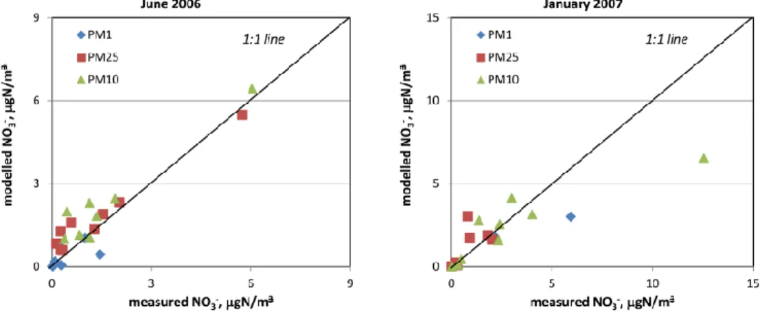
As discussed above, the model tends to somewhat over-predict nitric acid concentrations in June 2006 compared to observations, while it under-predicts concentrations in Jan-uary 2007. During June 2006, nitrate is in general lower in the model results compared to hourly data, though less so at GB36. However, when all intensive data is considered, the model is in general higher than observations for nitrate in June 2006 (Fig. 9; Tables 2 and 3). There is a tendency that nitrate in PM1is less biased, and the model even show

lower concentrations than observations (Fig. 9), indicating that there is a somewhat too high formation rate of nitrate di-rectly from HNO3(supposed to account for the reaction on

sea salt and dust). In the winter, the modelled and measured levels of nitrate are in good agreement. These results are in agreement with what is found when the EMEP model results are compared to the ’standard’ EMEP measurements (Fagerli et al., 2011).

3.2.2 Ammonia and ammonium

For June 2006, both the modelled and measured diurnal cy-cle of NH3have a usually a maximum in early morning, and

in general somewhat higher NH3concentrations during day

time than night time, except at Ispra (IT01) where the mod-elled NH3show little diurnal variation. The same pattern can

be found for January 2007, although the diurnal variation is somewhat weaker in the measurements, and somewhat more pronounced in the model results. The diurnal cycle of ammo-nia is governed by several factors like (1) the diurnal cycle of the emissions, (2) the conversion to ammonium (ammonium nitrate and ammonium sulphate) and (3) dry deposition and atmospheric stability. Agricultural sources tend to emit more ammonia during day time (due to e.g. higher temperatures, more wind/mixing), thus for sites that are close to source ar-eas, the stronger source during day time may outcompete the larger boundary layer mixing. This is not exactly reflected by the variation of NH3in NL11, as the average highest

con-centrations are seen at night and most pronounced in June. This may be due to nearby farms with forced ventilation, which emit the same quantity at day and night. With a thinner mixing layer at nighttimes the regional concentration will be higher. However, it should be noted that a strong NH3peak

during a single night (from 19 to 20 June), caused these high average concentration during night, whereas the median diur-nal cycle of NH3shows the expected peak in early morning

Fig. 8. Diurnal variations of gaseous and particulate nitrogen species from some of the intensive measurements compared with the EMEP model. Measured ammonium and nitrate in PM2.5at Cabauw (NL11) and Harwell (GB36) while in PM10at Ispra (IT04) Note: there are two curves showing model results of nitrate at Cabauw and Harwell: for ammonium nitrate (NH₄NO₃) (red) and nitrate in PM₁₀, (mod NO3) which is the sum of NH4NO3and coarse NO−₃ (black) (see explanations in Sect. 3.2.1).

Fig. 9. Modelled and measured nitrate in the different size fractions for June 2006 (left) and January 2007 (right). Note different scale for the two periods.

8090 W. Aas et al.: Lessons learnt from the first EMEP intensive measurement periods hours at NL11 (as in the model results) as seen when

av-eraging for a complete year (Schaap et al., 2011). In the EMEP model, we assume that emissions during day time are a roughly a factor of two higher than at night time throughout the whole year. In reality, the day-night variation might be very different from site to site, depending e.g. on the type of agricultural sources and the meteorology. In order to provide a better diurnal variation of ammonia emissions (and thus also for ammonia concentrations) the EMEP model could be coupled to a dynamic, mechanistic ammonia emission model where the diurnal variation of emissions would depend on temperature, wind and type of agricultural activity. Such an emission module has already been implemented for Denmark and the extension to a European module is on its way (Skjøth et al., 2011). Similarly, the introduction of a bi-directional ex-change module (Massad et al., 2010) would result in higher NH3 concentrations during the day when deposition is

re-duced due to elevated compensation points.

The modelled diurnal cycle of ammonium at Cabauw (NL11) and Harwell agrees well with measurements with the highest values found at night (similarly as nitrate) (Fig. 8). At Auchencorth Moss (GB48), June 2006, measured ammo-nium is found to peak in early afternoon at the same time as NH3 peaks. In the model however, ammonium peaks in

early morning. The failure to describe ammonium at this site is probably due to the failure to describe the NH3ammonia

emission diurnal variability. In January 2007, however, the diurnal cycle of modelled and measured ammonium agree well, although the level of ammonium is somewhat over-predicted by the model compared to observations. Both mea-surements and model results show a peak in the early morn-ing. At Ispra (IT04) the model on the other hand is lower than the measurements and the diurnal variation is less pro-nounced that at the other sites, similar as the general ten-dency as discussed for the filter measurements (Table 3 and 4).

4 Conclusion

EMEP 2006 and 2007 IMPs have produced a set of valuable data which has given new insights and improved our under-standing regarding composition of particulate matter in dif-ferent size fractions, seasonal and geographical differences, gas/aerosol partitioning and diurnal variations. The size seg-regated and chemically resolved PM measurements and the hourly measurements of gaseous and aerosol species which is not part of the regular EMEP measurement program has led to new possibilities for validation of the EMEP model.

In general, the model has been shown able to reproduce the main features of PM composition, spatial and tempo-ral (summer-winter) variation, though discrepancies between measured and calculated PM have also been found. The availability of PM chemical composition measurements has facilitated a more profound analysis of PM results. Among

others, the intensive measurement data has identified im-provements needed for increasing the accuracy of the EMEP model aerosol calculations. In particular, size-distribution and formation rates of HNO3 and coarse nitrate. Explicit

modelling of the sea-salt and dust reactions will be intro-duced in future in order to address some of these factors, and more size-resolved measurements of nitrate and other compounds is needed to evaluate such changes properly. Fur-thermore, the diurnal variation of ammonia would proba-bly improve if the EMEP model is coupled to a dynamic, mechanistic ammonia emission module. The model results for sulphate aerosol have been significantly improved; still its tendency to underestimate sulphate should be further in-vestigated, making also use of hourly measurements. Part of model underestimation of EC, at central and south European sites is probably due to emission uncertainties. Similarly, OC tends to be underestimated at southern sites, suggesting that residential wood burning source is underestimated in winter (Bergstr¨om et al., 2012; Denier van der Gon et al., 2012). It should be noted that both primary and secondary OC has been included in the calculations for the first time, showing promising results (Bergstr¨om et al., 2012). The lack of mea-surements of mineral dust hamper the possibility for model evaluation for this highly uncertain PM component, and it is strongly recommended that more sites measure the full set of mineral components (Querol et al., 2011).

It is well known that chemical speciation measurements can be biased, especially for nitrogen and organic species, and the intensive measurements clearly showed that the lack of comparability between datasets makes it difficult for re-gional assessments and comparison with models. Artefact free methods like continuous measurements and denuders should be applied especially during campaigns like this. It is also apparent that a standardized method is needed to get comparable data for EC and OC, either by using a centralised lab or by agreeing upon a common protocol, even though not perfect. These issues were taken into account during the sec-ond intensive measurement period, which was csec-onducted in October 2008 and March 2009. I.e. these periods included centralised laboratories for levoglucosan and 14C, and all labs measuring EC/OC followed the same protocol (Yttri et al., 2012; Cavalli et al., 2010).

There are relatively large uncertainties in both measured and modelled estimates, but to quantify this is very dif-ficult. The main reasons for model uncertainty are uncer-tainties in input data (e.g. emissions, meteorology, landuse, etc.) and uncertainties in processes descriptions in the model. The accuracy of model calculations varies a lot for differ-ent PM compondiffer-ents, with SIA aerosols being better under-stood (though still far from being perfectly represented by the model), while SOA and windblown dust being rather uncer-tain. In the measurements, the uncertainties are both related to measurement method itself and the performance of the analysis. For further details on the uncertainty in assessment