Static code metrics vs. process metrics for software fault prediction using Bayesian network learners

(1)

Static code metrics vs. process metrics for

software fault prediction using Bayesian

network learners

Mälardalen University

School of Innovation, Design and Technology

Author: Biljana Stanić

Thesis for the Degree of Master of Science in Software Engineering (30.0 credits)

Date: 28th_{October,
2015}

Supervisor: Wasif Afzal

Examiner: Antonio Cicchetti

(2)

“The real question is not whether machines think but whether men do.

The mystery which surrounds a thinking machine already surrounds a

thinking man.”

Burrhus Frederic Skinner

(3)

Acknowledgments

I would like to express my deep appreciation to my supervisor, Dr. Wasif Afzal, for the constructive, useful suggestions, and guidelines throughout my research work.

I would also like to thank to:

EUROWEB Project1_{,
funded
by
the
Erasmus
Mundus
Action
II
programme
of
the}

European Commission;

Lech Madeyski and Marian Jureczko for using their metrics repository.

Finally, I wish to thank my dear ones for their support and for believing in me all this time. 1_{http://www.mrtc.mdh.se/euroweb/}

(4)

Abstract

Software fault prediction (SFP) has an important role in the process of improving software product quality by identifying fault-‐prone modules. Constructing quality models includes a usage of metrics that describe real world entities defined by numbers or attributes. Examining the nature of machine learning (ML), researchers proposed its algorithms as suitable for fault prediction. Moreover, information that software metrics contain will be used as statistical data necessary to build models for a certain ML algorithm. One of the most used ML algorithms is a Bayesian network (BN), which is represented as a graph, with a set of variables and relations between them. This thesis will be focused on the usage of process and static code metrics with BN learners for SFP. First, we provided an informal review on non-‐static code metrics. Furthermore, we created models that contained different combinations of process and static code metrics, and then we used them to conduct an experiment. The results of the experiment were statistically analyzed using a non-‐parametric test, the Kruskal-‐Wallis test.

The informal review reported that non-‐static code metrics are beneficial for the prediction process and its usage is highly recommended for industrial projects. Finally, experimental results did not provide a conclusion which process metric gives a statistically significant result; therefore, a further investigation is needed.

(5)

List of Figures

Figure 1. Example of NB [6] ... 19

Figure 2. Example of STAN [6] ... 20

Figure 3. Methodology for the RQ1 ... 22

Figure 4. Methodology for the RQ2 ... 24

Figure 5. Weka Explorer ... 30

Figure 6. Set values for NB classifier ... 31

Figure 7. Classifier output with results ... 32

Figure 8. Graphs with comparison results for NB classifier ... 42

Figure 9. Graphs with comparison results for TAN classifier ... 43

Figure 10. Graphical comparison of combined, static code and process models using NB ... 51

Figure 11. Graphical comparison of models containing 1 process and static code metrics using NB ... 51

Figure 12. Graphical comparison of models containing the combination of 2 process and static code metrics using NB ... 52

Figure 13. Graphical comparison of models containing the combination of 3 process and static code metrics using NB ... 52

Figure 14. Graphical comparison of combined, static code and process models using TAN ... 53

Figure 15. Graphical comparison of models containing 1 process and static code metrics using TAN ... 53

Figure 16. Graphical comparison of models containing the combination of 2 process and static code metrics using TAN ... 54

Figure 17. Graphical comparison of models containing the combination of 3 process and static code metrics using TAN ... 54

(8)

List of Tables

Table 1. Selected projects for the experiment ... 27 Table 2. Results for combined, static code and process metric using NB classifier ... 34 Table 3. Comparison results for combined, static code and process models for NB

classifier ... 34 Table 4. Results for models containing 1 process and static code metric using NB

classifier ... 35 Table 5. Comparison results for models containing static code and 1 process metrics

using NB classifier ... 35 Table 6. Results for models containing combination of 2 process and static code metrics

using NB classifier ... 36 Table 7. Comparison results for models containing combination of 2 process and static

code metrics using NB classifier ... 36 Table 8. Results for models containing combination of 3 process and static code metrics

using NB classifier ... 37 Table 9. Comparison results for models containing combination of 3 process and static

code metrics using NB classifier ... 37 Table 10. Results for combined, static code and process models using TAN classifier ... 38 Table 11. Comparison results for combined, static code and process models using TAN

classifier ... 38 Table 12. Results for models containing 1 process and static code metrics using TAN

classifier ... 39 Table 13. Comparison results for models containing static code and 1 process metrics

using TAN classifier ... 39 Table 14. Results for models containing combination of 2 process and static code metrics using TAN classifier ... 40 Table 15. Comparison results for models containing combination of 2 process and static

code metrics using TAN classifier ... 40 Table 16. Results for models containing combination of 3 process and static code metrics using TAN classifier ... 41 Table 17. Comparison results for models containing combination of 3 process and static

code metrics using TAN classifier ... 41

(9)

Abbreviations

SFP Software Fault Prediction ML Machine Learning

BN Bayesian Network DAG Directed Acyclic Graph

NB Naive Bayes

ANB Augmented Naive Bayes TAN Tree Augmented Naive Bayes

FAN Forest Augmented Naive Bayes STAN Selective Tree Augmented Bayes STAND Selective Tree Augmented Bayes with

Discarding

SFAN Selective Forest Augmented Bayes SFAND Selective Forest Augmented Bayes with

Discarding

ANOVA Analysis of Variance

WMC Weighted Methods per Class DIT Depth of Inheritance Tree NOC Number Of Children

CBO Coupling Between Object class RFC Response For a Class

LCOM Lack of Cohesion in Methods

LCOM3 Lack of Cohesion in Methods (normalized version of LCOM)

Ca Afferent Coupling Ce Efferent Coupling LOC Lines Of Code

(10)

DAM Data Access Metric MOA Measure Of Aggregation

CAM Cohesion Among Methods of class IC Inheritance Coupling

CBM Coupling Between Methods AMC Average Method Complexity

CC McCabe’s Cyclomatic complexity NR Number of Revisions

NDC Number of Distinct Committers NML Number of Modified Lines

NDPV Number of Defects in the Past Version ROC Receiver Operating Characteristic AUC Area Under the Curve

RQ Research Question RQ1 Research Question 1 RQ2 Research Question 2

(11)

1. Introduction

Introducing the term ‘software engineering measurement’ and its basic characteristics, creates a logical step for defining another one—software metrics. Software metrics represent numbers or certain attributes used for describing real world entities formed by definite rules. Moreover, there are certain software quality assurances that use such metrics. One of the activities involves constructing quality models based on metrics. In that manner, quality metrics are beneficial for determining if the software system delivers the intended functionality [1].

A software fault prediction (SFP) model is one type of the quality model that has attracted a lot of research in the past few decades [2]. Complexity of the system brings

mistakes in the code, labeled as faults2_{[16],
and
their
discovery,
as
the
system
grows,
is}

not an easy task for the developers [3]. The process of detecting faults can be long and infinite, since it is hard to claim that a system is 100% fault-‐free. This also requires additional resources during testing which leads to enlarging costs of software development. One of the solutions is the creation of a prediction model that will guide development team towards quicker and more efficient fault detection [3]. With the help of metrics, it is possible to define a model that is responsible for predicting faults. Hall et al. [4] claim that there are a lot of complex models that deal with the problem of fault prediction, but despite that, there is a visible lack of information about the actual state in this area.

Song et al. [2] list three most researched problems in SFP. These problems are:

o Determining the number of faults that were not identified during testing;

o Finding connections between remaining faults and;

o Classification of components that are fault-‐prone.

To solve above mentioned problems, a lot of attention in the past has been on applying machine learning techniques. Machine learning (ML) is about programming machines in order to get optimized results using statistical data or previous experience. ML uses statistical rules to build different mathematical models necessary for creating a conclusion from a sample [15]. The nature of ML, and some of its algorithms, is suitable for a creation of fault prediction models, which has shown good results. ML algorithms use patterns to identify and classify features, e.g., whether a software component contains a fault or not. One of the mostly used ML algorithms is a Bayesian network (BN) [2]. The BN is represented through a directed acyclic graph (DAG) containing set of variables, a certain structure that is defined as a relation between variables and a set of probability distributions. For the cases, such as software products, the usage of the BN can be depicted as a relationship between software features and possible faults. The network can be used for computing probabilities of the presence of different faults for specified features. That way, we will know which faults are possible to occur and how we can control and isolate them [5].

(12)

1.1 Motivation

The main arguments for this thesis are found in recent publications [6],[7], where the usage of BNs has been found to be performing “surprisingly well” [6].

Dejaeger et al. [6] conducted experiments where different BN learners with static code metrics were compared. They made this choice of metrics because they are easier to gather and they are widely used in practice. They recorded better prediction for cases where a smaller set of features, that are highly predictive, were used. For the future work, they stated:

“Recently, several researchers turned their attention to another topic of interest, i.e., the inclusion of information other than static code features into fault prediction models such as information on intermodule relations and requirement metrics. The relation to the more commonly used static code features remains however unclear. Using, e.g., Bayesian network learners, important insights into these different information sources could be gained which is left as a topic for future research.” [6]

This conclusion represents the starting point and the main motivation for the thesis definition. Dejaeger et al. [6] indicated that one interesting direction of investigating BN learners for SFP is to include non-‐static code metrics. They are proposing information on intermodule relations and requirement metrics. These two are just examples of many other non-‐static code metrics that can be used for SFP.

Another paper that deals with BNs for SFP, and gives a great motivation, is by Okutan et al. [7]. For the experiment, they reported performance of some static code metrics. Namely, they stated that metrics with information about a number of lines of code (LOC), low quality of a coding style and a class response were the most effective. Moreover, they presented other conclusions of their experiment and possible steps for an extension of their research:

“As a future direction, we plan to refine our research to include other software and process metrics in our model to reveal the relationships among them and to determine the most useful ones in defect prediction. We believe that rather than dealing with a large set of software metrics, focusing on the most effective ones will improve the success rate in defect prediction studies.” [7]

Following the statement in [6], Okutan et al. are proposing the usage of process metrics.

Radjenović et al. [8] have done a systematic literature review on SFP metrics and collected results that are supporting statement given in [7] about process metrics and their future usage for fault prediction. They came up with the following conclusions:

o Process metrics have shown better results in detecting faults on post-‐release

level than static code metrics;

o Process metrics, comparing to static code metrics, contain more descriptive

information related to fault distribution;

(13)

o Unlike object-‐oriented metrics that are mostly using small datasets, process metrics are applicable for larger datasets and it is an advantage when it comes to the validity and maturity of research results [4];

o Process metrics can be very beneficial, but they are mostly used in industrial

domain. Therefore, it is challenging for researchers to use process metrics in their studies in the future.

1.2 Research questions

Taking into account the collected statements about SFP, BNs and the usage of non-‐static code metrics, the structure of the thesis will be defined by the research questions:

o RQ1: What is the current state-‐of-‐the-‐art with respect to the use of non-‐static code metrics for SFP?

o RQ2: What is an impact of process metrics combined with static code metrics, in terms of performance, using BN learners for SFP?

In RQ1, we will discuss and explain in detail the current state-‐of-‐the-‐art of non-‐static code metrics, with a focus on process metrics. Research will be driven by conclusions made by Radjenović et al. [8]. For RQ2, we will be conducting experiments where several process metrics are combined with static code metrics and they will be used with BN learners. The results of this thesis can give a new insight into software metrics

that can be beneficial for SFP.

The content of the thesis is organized as follows: Section 2 contains background information about SFP, software metrics, ML and BN. Section 3 explains the method for collecting resources for the informal review and the experiment. In Section 4, informal review on non-‐static metrics will be presented. Section 5 contains information about the design of the experiment, used datasets and a response variable. In Section 6, results of the experiment and statistical analysis will be presented. Moreover, Section 7 provides a discussion of a comparison of experimental outcomes. Section 8 explains possible validity threats. Finally, Section 9 offers conclusions and lists areas of future work.

(14)

2. Background

In this section, we will describe SFP, the purpose of software metrics, how ML can be used for fault prediction (with a focus on BN learners).

2.1 Software fault prediction

SFP, as quality model, is recognized as an important tool for improving software product by identifying possible faults that can occur in the system. Faults directly jeopardize software, which decreases its performance, and, furthermore, its quality [16].

Software systems are designed to handle complex activities in different domains. Because of their critical nature, every system is supposed to provide quality of service for its users. As the system increases, the growth of potential faults enhancements. Dejaeger et al. [6] found several cases where software faults were examined in terms of reliability and bug localization. In order to test reliability, we need to create a stochastic model that will output probability of fault existence once the component is executed. Combining remaining components, we are able to estimate the reliability of the whole system. Bug localization is based on usage of certain patterns that are associated with faulty components. Using this approach, we can discover faults that were not previously detected [6].

We saw that it is crucial to classify and identify fault-‐prone modules of the software on time. Different studies in this area have shown that faults, in majority cases, occur just in several modules and it causes malfunctioning of the other parts of the system and, also, those that are in direct relation with faulty ones. This means that the costs of production and maintenance will increase due to the effect of faults in these modules [9]. Therefore, much research has been focused on making fault prediction regarding system under development. Such predictions focus on locating modules that can be shown to be fault-‐ prone [10]. Thus, creating accurate predictions is useful for increasing the quality of the system [9].

To be able to achieve good results, software engineers have to find a suitable prediction technique that will help them in their intention of detecting faults and conducting experimental validation [10]. Since direct measurement of fault prediction is impossible, we need to use metrics for necessary estimation. Reliable results of prediction depend on selection of software metrics. One needs to select appropriate metrics, because there exists a number of datasets that can make a prediction harder and might result in unsatisfactory and misleading results.

Once the metrics are chosen, it is necessary to decide which technique will be used for

making predictions. ML is the non-‐parametric3_{technique
that
is
frequently
used
for
SFP.}

Sometimes datasets can be heavily skewed, which results in inaccurate prediction. ML techniques have a mechanism to overcome such problems, because it has an ability to “learn from imbalanced datasets” [11].

In Section 2.2, we will describe software quality metrics and ML as key elements in SFP process.

3_{distribution-‐free}

(15)

2.2 Software metrics

Software quality metrics deserve particular attention in SFP since they can be used for measuring quality of the system. They are further divided into in-‐process and end-‐ process metrics. The first group of metrics is responsible for improving the development process, unlike end-‐process that is focused on assessment of the characteristics of the final product.

Based on measuring specific parts of the system, there can be two types of software quality metrics:

o Static;

o Dynamic metrics.

Static code metrics are suitable for checking attributes of the code, such as the complexity of the software and accessing the length of the code. Dynamic code metrics in a great extent examine the behavior of the system, presented as usability, reliability, maintainability and evaluation of the efficiency of the program [6].

In Section 2.2.1, we will briefly introduce some metrics, namely static code and process, which are relevant for the further content of this thesis.

2.2.1 Static code metrics

Static code metrics are a type of quality metrics. Their usability is noticeable when it comes to measuring:

o Size (through lines of code (LOC) counts);

o Complexity (using linearly path counts);

o Readability (through operator counts and different operands).

The principle of calculating static code metrics is based on parsing of the source code; therefore, the process of metrics collection is automated. Because of this feature, it is manageable to measure metrics of the whole system, regardless of the system’s size. Moreover, it is possible to make predictions about the entire system based on metrics— developers can easily find faulty modules since they have a clear image of system’s vulnerabilities [12]. Static code metrics are easier and widely used in practice; therefore, they are representing a safe choice for predicting faulty software [6].

2.2.2 Process metrics

Process metrics are also used for measuring the quality of the system [8]. They can be specified from various sources:

o Developer’s experience [10];

o Software change history [8], etc.

Developer’s experience is concentrated on activities that are envisaging how a certain part of the code (or the whole system) was developed [10].

Those metrics that are determined through the software change history split into two groups:

o Delta;

(16)

Delta metrics are defined as the difference between versions of the software [8]. As the result, we have the changed value of the metrics from one version to another. An illustrative example is when we are adding new lines of code and when we save those changes, delta value will be different. In cases when we are adding, and at the same time removing the same number of lines of code, delta value between those two versions will be the same. To be able to track changes, code churn metrics will report every activity on the code.

Advantage of using process metrics is that they contain more descriptive information about a faulty part of code. They are also good at making fault predictions on post-‐ release level. Since process metrics are used mostly for industrial purposes, they are able to handle large datasets, which leads to better validity of the predictions [8].

2.3 Machine learning

ML is about programming machines in order to get optimized results using statistical data or previous experience. ML uses statistical rules to build different mathematical models necessary for creating the conclusion from the sample [15]. Those models can give predictions of the future steps or form a description based on knowledge from different data, or combining both in particular cases [15]. The first step for building the model is to train data using certain algorithms in order to optimize the specified problem. Learned model has to be efficient in terms of time and space complexity.

ML has several applications in:

o Learning Associations; o Supervised learning; o Unsupervised Learning; o Regression; o Reinforcement Learning.

We will use real-‐life examples to explain types of ML.

Learning Associations are suitable for “learning a conditional probability”. Probability is presented in equation 1:

𝑃(𝑋) (1)

where Y is a variable that is conditioned on X. Moreover, X can be a single or a set of variables of the same type as Y. Taking the example of a bookstore; Y can be a book that we are conditioning on X. Based on customer's behavior, we know that when s(he) buys a book from X, there is a high probability that Y will we bought as well.

In supervised learning input features are related to corresponding outputs and machine has to understand rules of mapping between those two parameters. Supervised learning is applicable for prediction tasks, where is necessary to identify connections between different measures. On the other hand, for unsupervised learning, output data are not required, however, it examines structure within some input dataset. Unsupervised learning is not suitable for predictions of existence software faults in the

(17)

system because of its nature to create the result without previously specified output data.

Cases of supervised learning problems are classification and regression. In classification, we are making predictions based on a rule learned from the past data. Assuming that a behavior is similar in the past and future, we can easily produce predictions for every future case. The input contains data that we need to analyze, whereas the output is represented as classes that have a descriptive value.

Regression has the same approach for selecting the input data as the classification problem, but for the output we will get a numerical value. In classification and regression problems we are creating the model, shown in equation 2:

𝑦 = 𝑔(𝑥|𝜃) (2)

where y is the class, in classification, or the numerical value, in regression. The model is

represented as g (._{)
and
model’s
parameters
as
𝜃.
The
task
of
ML
is
to
optimize
values
of}

𝜃, in order to get a minimized approximation error.

Reinforcement Learning has for the input set of actions. In that system, it is important that all actions are part of a “good policy” [15], which will lead to obtaining correct results. In this particular problem, we are not observing a single action. The task of the program is to learn with characteristics are forming the good policy based on past set of actions [15].

Finally, ML has a mechanism to overcome problems of datasets that are heavily skewed and that can cause inaccurate results [11]. This basically means that it possible to create prediction even if some data are missing, or there is a big number of variables, etc. [17].

The BN is a type of supervised learning paradigm and one type of algorithm suitable for SFP (see Section 2.3.1).

2.3.1 Bayesian network

The structure of a BN is presented as a directed acyclic graph (DAG) consisting of variables, a certain structure that is defined as a relation between variables and a set of probability distributions [5]. Considering the nature of SFP, BN can be used for calculating probabilities regarding the presence of faults in the software features.

The BN graphically presented as a graph, contains following elements:

o Variables that are presented as vertices or nodes;

o Conditional dependencies that are edges or arcs.

This graph cannot contain cycle and all edges inside it have to be directed. BNs provide theoretical framework that combined with statistical data, can give good fault predictions [5]. Model for SFP can be defined as (see equation 3):

𝐷 = 𝑡𝑟𝑛 { 𝑥_!, 𝑦_! }_!!_{= 1} ₍₃₎

(18)

where D is a set with N observations, with 𝑥_! ∈ 𝑅!_{shows
all
static
and
non
static
code}

features and 𝑦_! ∈ {0, 1} is used to indicate presence of some fault.

Using Bayesian theorem for the BN to calculate probability of fault presence, we will have the following equation 4:

𝑃 𝑦_! = 1|𝑥_! = 𝑃 𝑥!|𝑦! = 1 𝑃(𝑦! = 1)

𝑃(𝑥_!) (4)

The concept of the BN is based on probability distribution using stochastic variables that

can be both continuous and discrete. Individual variables 𝑥(!) are used to construct the

graph and dependencies between those variables are presented with directed arcs. In

the same way, independence between different nodes 𝑥_(!) and 𝑥_(!!) is shown by the

absence of the arc [6].

Defining and building the BN consists of three steps [14]:

o “Set” and “field” variables have to be defined;

o Network topology has to be constructed;

o Probability distribution on the local level has to be identified.

Set and field variables have to be defined

“Set” variable inspects possible factors that are causing software faults, while “field” variable has to change the range of all variables to the degree of software faults. The value of “set” variable can vary depending on the system, organization, environment where it will be used. Variable “field” can be stated as “high”, “middle” or “low” (or more precise if it is required).

Network topology has to be constructed

Network topology is defined using event relation. The construction of the certain topology depends on studies or literature and it can be changed if experiments demand it.

Probability distribution on the local level has to be identified

In order to identify probability distribution on the local level, it is required to find marginal and conditional probabilities. Probability distribution can be used to emphasize “affect degree of causality” [14].

BN classifiers are used for problems that require classification. Other attractive features that classifiers have are presented in following list:

o Models can be created even if the knowledge is uncertain;

o Probabilistic model can be used for cost-‐sensitive problems;

o The nature of BNs classifiers can deal with issues related to data that are missing;

o Classifiers can solve complex classification problems;

o Future work on BNs include presenting models in hierarchical manner based on

their complexity;

o There is possibility of using BN classifiers with algorithms that have linear time

complexity;

(19)

In Section 2.3.1.1, we will present 2 types of BN learners (classifiers) what will be used for the experiment.

2.3.1.1 The Naive Bayes Classifier

The Naive Bayes (NB) is based on “conditional independence between attributes given the class label” [6], which is represented with nodes in directed acyclic graph, where one node is a parent and the rest are children. The node is a certain value in the dataset. Results from different studies have shown that NB classifiers are giving good results in fault prediction.

In order to calculate fault probability for classes, each of them will have a vector of input variables for every new code segment. Resulted probabilities are gained using “frequency counts for the discrete variables and a normal or kernel density-‐based method for continuous variables”. Because of their simplified nature, NB classifiers can be constructed very easily, containing computational efficiency. The structure of NB is shown in Figure 1 [6].

Figure 1. Example of NB [6]

As we have shown on Figure 1. NB consists of one unobserved parent variable (node y) and a number of observed children variables (x nodes).

2.3.1.2 Augmented Naive Bayes Classifier

Augmented Naive Bayes (ANB) classifiers were created as a modification of the basic conditional independence assumption principle of the NB. We will show changes in the graph that are made by adding new arcs and removing unnecessary variables. One

(20)

example of ANB classifier is the Tree Augmented Naive Bayes (TAN), where each variable has one more parent. On the other hand, Semi-‐Naive Bayesian classifier “partitions the variables into pairwise disjoint groups”. Finally, Selective Naive Bayes, in order to face correlation between attributes, omits some variables.

There are several ANB classifiers:

o Tree Augmented Naive Bayes (TAN);

o Forest Augmented Naive Bayes (FAN);

o Selective Tree Augmented Naive Bayes (STAN);

o Selective Tree Augmented Naive Bayes with Discarding (STAND);

o Selective Forest Augmented Naive Bayes (SFAN);

o Selective Forest Augmented Naive Bayes with Discarding (SFAND).

Graphical representation of the STAN is shown on the following Figure 2.

Figure 2. Example of STAN [6]

In Figure 2, is it shown that each child (x) node is allowed to have additional parent, located next to the certain class node. We will use the NB to balance the BN classifiers and show a clear image of all dependencies between attributes [6].

(21)

3. Method

This thesis will consist of 2 parts, depending on RQs. We will answer RQ1 by doing the informal review of the field and for RQ2 we will conduct the experiment.

3.1 Methodology for RQ1

In order to answer RQ1, we have to collect material related to:

o SFP;

o Metrics;

o ML and

o BN;

Our goal is not focused on conducting a systematic literature review on the topic of SFP, software metrics or ML and its algorithms, since it has already been done in several studies. Therefore, we will use collected sources to present the state-‐of-‐the-‐art for non-‐ static code metrics in the process of SFP.

Furthermore, in this section, we will describe the procedure that was followed in the process of selecting papers relevant for the thesis topic:

Step 1: Define keywords relevant for the RQ1:

o SFP;

o Software defect prediction;

o Code metrics;

o ML;

o BN.

Step 2: Define filters in terms of publication years and type of the papers

Selected papers are published between 2010 and 2015 and each of them has to be a journal or/and conference paper. The 5–year range was set to review only recently published results, which also include some recent literature reviews on the topic.

Step 3: Use keywords and filters in several databases:

o IEEExplore4_;

o ACM Digital Library5_;

o Scopus6_{(used
for
validation
of
papers
that
have
been
found
in
first
two}

databases).

Step 4: Collect and select results

To get suitable results from databases, search string often contained combination of terms, using Boolean AND and OR operators, such as:

(TITLE-‐ABS-‐KEY AND TITLE-‐ABS-‐KEY) AND DOCTYPE(ar OR re) AND ( LIMIT-‐

TO(SUBJAREA ) AND RECENT()7_.

4_{http://ieeexplore.ieee.org/Xplore/home.jsp} 5_{http://dl.acm.org/}

6_{http://www.scopus.com/}

(22)

Papers with SFP and process metrics keywords, found in Scopus database, were used for snowball sampling and collecting other papers relevant for this topic with the, earlier mentioned, 5–year range.

During the selection process, papers that were irrelevant, but have been displayed in search results, were rejected and other new papers were taken into consideration. The majority of papers were found in IEEExplore database.

Step 5: Present the informal review.

Present all relevant information regarding non-‐static code metrics.

In Figure 3, we will illustrate the activities as part of methodology for answering RQ1.

Figure 3. Methodology for the RQ1

(23)

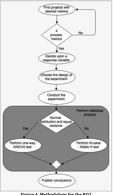
3.2 Methodology for RQ2

We identified following activities, suggested in [15], for finalizing RQ2:

o Find suitable projects with datasets containing extracted static and process

metrics;

o Decide upon a response variable;

o Choose the design of the experiment;

o Conduct the experiment for the projects, using previously selected BN

classifiers;

o Compare results using a statistical analysis;

o Publish conclusions about results of the statistical analysis.

Step 1: Find suitable projects with datasets containing extracted static and process metrics

We will analyze datasets available on the Metric Repository8_{collected
from
different}

open-‐source projects. The datasets were used in the study of Madeyski et al. [18].

Step 2: Decide upon a response variable

As the quality measure, we will use area under the curve, AUC, proposed in [6]. AUC is specified by an average value of performances defined by all thresholds.

Step 3: Choose the design of the experiment

A principle of our experimental design will be based on replication [15], which means that the experiment will be run a defined number of times in order to find an average value of the specific quality measure. More specifically, we will use cross-‐validation.

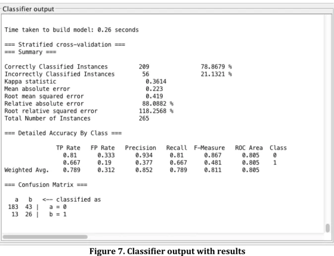
Step 4: Conduct the experiment for the projects, using previously selected BN classifiers As it is presented in the Background Section, for the purposes of the experiment, we will use NB and TAN classifiers. Using specified classifiers with the datasets, we will create a learner. Doing training multiple times and then testing with the validation sets, we will get results for the desired measure [15]. Implementation of classifiers is available

through Weka9_{,
suggested
in
[6],
which
will
speed
up
the
process
of
collecting
results
of}

prediction for the chosen datasets.

Step 5: Compare results using a statistical analysis

Conducting the statistical analysis of data is done for the reason of providing objective and unbiased results regarding the comparison of different datasets. Since we are operating with 17 datasets and 2 classifiers, we will decide between a one-‐way analysis of variance (ANOVA) or Kruskal-‐Wallis test, once we collect results from the experiment.

Step 6: Publish conclusions about results of the statistical analysis

The statistical analysis will give answers whether samples of the datasets are significantly different or not. In case we have differences, we will discuss which datasets are more superior to others, otherwise we will give an explanation and possible improvements for the future experiments.

8_{http://purl.org/MarianJureczko/MetricsRepo}

(24)

In Figure 4, we will illustrate the activities as part of methodology for answering RQ2.

Figure 4. Methodology for the RQ2

We will describe the experiment with detailed requirements in Section 5: Design.

(25)

4. Informal review

We collected recent papers that are dealing with SFP using non-‐static code metrics, in order to answer RQ1. The best source of information is found in a form of a systematic literature review and studies, which objectives were to investigate the performances of process metrics for various open-‐source, industrial projects and software systems. We classified relevant findings into several groups based on their occurrence in the papers. The groups are following:

o Process metrics in general;

o Code churn metrics;

o Developer metrics;

o Other process metrics.

4.1 Process metrics

In their systematic literature review, Radjenović et al. [8] analyzed 106 papers concluding that process metrics are represented only 24% among other metrics for the purposes of fault prediction. Moreover, they identified that process metrics, such as the number of different developers that worked on the same file, the number of changes made on some file, the age of a module, etc., are better for faults detection in post-‐ release phase of software development than some static code metrics. Those metrics are mainly produced extracting source code and the history from the repository. Results gained from different studies have pointed out several advantages of process over static code metrics:

o Process metrics provide a better description regarding distribution of faults in

the software;

o Used for Java-‐based applications, process metrics can provide better models in

terms of cost-‐effectiveness;

o Process metrics performed the best in cases of prediction faulty classes using

the ROC area.

However, some studies have shown that process metrics have not performed well because they were used in a pre-‐release phase of software development. Results of the conducted experiments have confirmed that process metrics perform better and have to be used in post-‐release phase, which explains previously mentioned issues in prediction [8]. In [4] is suggested combination of code, process and static metrics for the better prediction.

Xia et al. [20] analyzed performances of code and process metrics for the TT&C software. They emphasize the benefits of process metrics during different development phases, such as requirements analysis, design and coding. There have been listed 16 process metrics, suitable for the specific phase. In the early stages of software development, analysis of requirements and their maturity are metrics related to detection of faulty software module. Therefore, it is important to eliminate errors that occur in the requirements phase, which can be transferred to other stages of development, i.e. design and coding phases. Another important feature of process metrics is tracking historical