VTI meddelande 849A • 1998VTI meddelande 849A • 1998VTI meddelande 849A • 1998VTI meddelande 849A • 1998VTI meddelande 849A • 1998
EMV – a PC program for
EMV – a PC program for
EMV – a PC program for
EMV – a PC program for
EMV – a PC program for
calculating exhaust emissions
calculating exhaust emissions
calculating exhaust emissions
calculating exhaust emissions
calculating exhaust emissions
from road traffic
from road traffic
from road traffic
from road traffic
from road traffic
Program description and user guide
VTI meddelande 849A · 1998
EMV - a PC program for calculating exhaust emissions from
EMV - a PC program for calculating exhaust emissions from
EMV - a PC program for calculating exhaust emissions from
EMV - a PC program for calculating exhaust emissions from
EMV - a PC program for calculating exhaust emissions from
road traffic
road traffic
road traffic
road traffic
road traffic
Program description and user guide
Program description and user guide
Program description and user guide
Program description and user guide
Program description and user guide
Publisher: Publication:
VTI meddelande 849A
Published:
1998
Project code:
80051
SE-581 95 Linköping Sweden
Printed in English 2000
Project:
A calculation model for exhaust emissions from cars
Author: Sponsor:
Ulf Hammarström and Bo O. Karlsson Swedish Environmental Protection Agency
Title:
EMV – a PC program for calculating exhaust emissions from road traffic
Program description and user guide
Abstract
A PC program named EMV has been developed for describing total exhaust emissions from road traffic on a national or regional level. The model is used by the Swedish Environmental Protection Agency and the Swedish National Road Administration for reporting and monitoring total exhaust emissions from road traffic.
The program is specially designed to evaluate changes relating to traffic, the vehicle fleet and use of different fuel types and fuel qualities.
Foreword
As part of a commission received from the Swedish Environmental Protection Agency – "Calculation model – Vehicle exhausts" – the Swedish National Road and Transport Research Institute (VTI) has developed a PC based computer program with its associated program documentation and user guide. Work was managed by a group comprising:
• Larsolov Olsson, Swedish Environmental Protection Agency
• Erik Kutscher, Motor Test Center (MTC), Swedish Motor Vehicle Inspection Co
• Svante Nordlander and Håkan Johansson, Swedish National Road Admini-stration (VV)
• Ulf Hammarström, VTI
Inside VTI, work was allocated as follows:
• Ulf Hammarström, project management, model development and documen-tation
• Bo Karlsson, programming
• Siv-Britt Franke, typing of this document.
Apart from the user guide, this documentation also contains an outline program description.
At the prepublication seminar held at VTI, Reino Abrahamsson, Swedish Environmental Protection Agency, was the presenter.
The document has been translated by L J Gruber BSc(Eng) CEng MICE MIStructE.
Linköping, December 1998
Contents
Summary 9
1 Introduction 13
2 Outline program description 15
3 Technical issues 18
3.1 Installing EMV 18 3.2 Uninstalling EMV 18
4 Command buttons, general 19
5 Creating scenarios 20
5.1 Scenario list 20 5.1.1 Files included in the scenario 21
5.1.2 Vehicle definition 22 5.1.3 New scenario 23 6 Data files 25 6.1 File types 26 6.2 File list 27 6.3 File content 28 6.4 Item description 29 6.4.1 Traffic data 29 6.4.2 Vehicle description 31 6.4.3 Vehicle frequency 35 6.4.4 Distribution by legislation class 37 6.4.5 Annual mileage 39 6.4.6 Use of fuel 40 6.4.7 Fuel description 43 6.4.8 Scrapping 45
7 Correction files 47
7.1 Correction for humidity 47 7.2 Correction for cold start 48 7.3 Correction for fuel quality 49
8 Calculations 51
9 Output data 52
9.1 General output data 52 9.1.1 Exhaust emissions (Urban/Rural area) 53 9.1.2 Vehicle mileage per vehicle type and area 54 9.1.3 Exhaust emissions per vehicle type and fuel type 54 9.1.5 Effects per legislation class 55 9.2 Special output data 56 9.2.1 Warnings regarding extreme numbers of year models 56 9.2.2 Predicted number of year models in different years 57 9.2.3 Calculated vehicle mileage 58
11 Improvement and maintenance of EMV 61
EMV – a PC program for calculating exhaust emissions from road traffic
Program description and user guide by Ulf Hammarström and Bo O. Karlsson
Swedish National Road and Transport Research Institute SE-581 95 Linköping Sweden
Summary
The total exhaust emissions from road traffic cannot be measured: they must be calculated. Major shortcomings have occurred both in earlier calculation models and basic data. The model described here should lead to an improvement in the situation.
The goals set up by the Swedish Parliament regarding changes in emissions, for example nitrogen oxide, assume access to monitoring methods. If separate monitoring is performed for different parts of the community, the measure used must be the amounts of emissions, i.e. it is inadequate to work with percentage changes per sub-sector. The amounts per sub-sector must be summated to a total amount on the national level whose relative change can be compared with the goals set up by Parliament.
A traditional method of calculating emissions from road traffic is to use basic data in the form of traffic data and traffic-specific emissions. Such calculations can be performed with different ambition levels.
The need to improve monitoring of road traffic emissions is very great. The variety of methods and agencies hitherto involved has led to a variation in estimated reductions over a wide range, with extremes that may imply that the goals are either very far from being met or that they could have been met by a broad margin.
One of the aims of the EMV model described is to arrive at a method which can be accepted and used by a large number of organisations. Access to a usable data platform would thereby be improved, while discussions on what is correct or incorrect, at least those resulting from different definitions and forms of data, could be reduced.
The model is used to calculate and report emissions of the following substances: HC, CO, NOX, particulates, CO2, SO2 and Pb.
There are different ways of presenting these emissions:
• always including a division into vehicle types: car; light duty vehicle; bus; heavy truck with gross vehicle weight up to 16 tonnes; heavy truck with gross vehicle weight above 16 tonnes; moped and motorcycle
• area type, rural or urban
• engine type: gasoline; diesel; gas or alcohol • legislation class and engine type.
The total volumes of fuel are an important type of output data for validation and other purposes.
• Vehicle description • Vehicle frequency
• Distribution by legislation class • Annual mileage
• Use of fuel qualities • Fuel quality description • Scrapping.
Traffic data is given vehicle type by vehicle type and year by year and includes:
• short and long distance trips • with or without trailer • number of trips • mileage
• percentage of mileage in urban areas • load factor.
The reason for a split into short and long distance trips is that transport statistics are often presented in this way and the strong correlation to use of trailers, driving in urban areas and load factors.
Vehicle description includes:
• hot engine emissions: without or with trailer; rural or urban • cold start emissions
• evaporative emissions.
There could be individual deterioration factors given for hot engine, cold start and evaporative emission factors.
Different qualities of fuels can result in different emission factors by time. Use of trailers has a major influence on emission factors. This use can vary between regions and by time. For all vehicle types, except two wheelers, there are separate emission factors without and with trailers.
For all hot engine emissions there are load factor corrections which automatically result in adjustments based on input data load factors.
Vehicle frequency is needed vehicle type by vehicle type including:
• number of vehicles by year model • engine type distribution.
For each vehicle type this data is needed for at least two years. For all other years EMV will estimate vehicle frequency and engine type distribution.
Distribution by legislation class is needed since there could be different
classes for the same year model.
Annual mileage describes the use of a vehicle as a function of vehicle type,
engine type and vehicle age. This type of data could be expected to vary by time and there could be different data sets for different years.
Use of fuel qualities is used to describe that emission factors are measured for
one fuel quality and there are other emission factors for qualities in regular use. The use of other fuel qualities also vary with time. There are correction factors to adjust the basic emission factors for other fuel qualities than those used when the basic factors were measured.
Fuel quality description includes the content of nine important substances for
Phosphorus; Oxygenate; Ignition improver). Also fuel density is included in the description.
Probability of scrapping is used to describe vehicle frequencies for future
years.
Future year model distributions are calculated as a function of the most recently entered year model distribution, scrapping probability and traffic development.
The model calculates emissions down to a level formed by the combination: vehicle type, engine type, year model, legislation class and fuel quality.
The program is specially designed to evaluate changes relating to traffic, the vehicle fleet and use of fuel. What cannot be described directly are changes to the road network, traffic regulations and driving behaviour. If, for instance, the user wants to evaluate the effect of changes in speed limits, new values of "hot emission" must be produced elsewhere.
The same applies to "cold start" where the user may, for instance, wish to evaluate increased use of engine heaters. In such a case new cold starts or, in actual fact, correction factors must be calculated.
One main feature of EMV is its ability to describe that the same vehicle type, engine type, year model and legislation class could have different emission factors in different years as a function of: use of trailers; driving in urban areas; load factors; deterioration and fuel qualities used.
The model has been subjected to extensive testing. It is used by organisations such as the Swedish Environmental Protection Agency and the Swedish National Road Administration for reporting and monitoring total annual exhaust emissions from road traffic.
1 Introduction
What is the extent of the total exhaust emissions from road traffic, either regionally or nationally? The model described below, called EMV, can be used to answer questions of this type. Calculations can relate to either a historic or a future description. A historic description is required for monitoring the environmental targets of the Swedish parliament regarding e.g. CO2 from 1990
onwards, or in order to produce environmental statistics. It may be necessary to evaluate different future scenarios as the basis for an assessment of environmental and traffic policy decisions.
It is hoped that its user friendly and problem oriented program design will lead to a more general acceptance of EMV.
The demands imposed on the user of the computer program are minimal. It is sufficient to enter the desired calculation year for the associated base data file to be accepted. The more deviations there are from the base file which forms part of a calculation scenario, the more input will be required from the user. What is chiefly necessary is to develop alternative data, but also to have a knowledge of the EMV model itself. A fundamental principle in program writing has been that it shall be possible to see "all" calculation assumptions. One alternative would be to integrate data outside the model. It may, for instance, have been decided to choose the alternative of the Swedish National Road Administration (VV) for the emission factors of cars in the reference (Vägverket, 1993), with mean values within larger groups of cars with gasoline engines, as follows:
• the group of cars without catalysts, which has been chosen for models up to the year 1986 (A)
• the group of cars with catalysts representing a previous stage of technology, represented by the 1990 model (B)
• the group of cars with more advanced exhaust treatment technology, represented by the 1997 model (C).
Developments within Category A, between the different year models in the class, do not therefore appear different from the description in the base file in EMV. In the base file, developments for cars up to the 1986 model are described by five sets of emission factors.
With EMV, the user can choose which detailed description to employ within the constraints of the program. There is nothing against choosing the VV alternative. However, in the base file of EMV we have attempted to describe models of "all" years and "all" legislation classes, which was part of the wishes of the client.
The enclosed base file (Scenario 1) is a read-only document and cannot by mistake be altered by the user. The base file can be easily copied as a basis for the user's own scenarios. Special documentation is available with source references for all the input data used in the base file (Hammarström and Henriksson, 1997).
The program is specially designed to evaluate changes relating to traffic, the vehicle fleet and use of fuel. What cannot be described directly are changes to the road network, traffic regulations and driving behaviour. If, for instance, the user wants to evaluate the effect of changes in speed limits, new values of "hot emission" for the window Vehicle description must be produced elsewhere, for
instance with the computer program VETO1. The same applies to "cold start" where the user may, for instance, wish to evaluate increased use of engine heaters. In such a case new cold starts or, in actual fact, correction factors must be calculated with the program COLDSTART (Hammarström and Edwards, 1998). COLDSTART can also be used to calculate regionally adapted correction factors.
1 This program was documented in VTI Bulletin No 501. It was used in producing the emission functions used
2
Outline program description
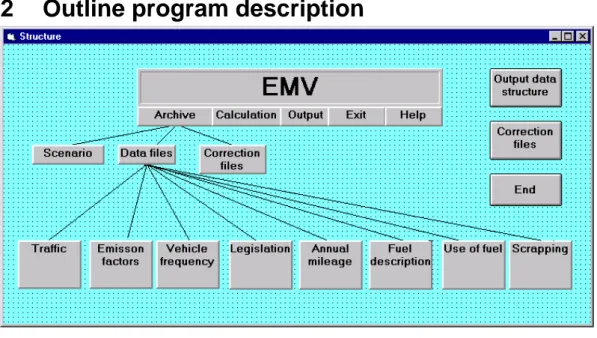
Fig. 2.1 Outline program structure.
An outline program description is given by the structure window under Help, see Fig. 2.1. The structure comprises:
• a file module
• a calculation module • an output data module • a help module.
The option End is also included. In principle, the file module is in two parts, a scenario part and a data file or correction file part. Scenarios are defined by the user on the basis of the data or correction files.
A calculation relates to emission during the year selected by the user, for the scenario selected.
The results of the latest calculation are always available under Output data. Under Output data, the user can choose between different types of output data.
One term that recurs in both Files and Calculation is Scenario. When a calculation is to be performed, it is made for a Scenario.
There are two groups of files: Data files and Correction files. There are eight different file types under Data files and three under Correction files.
A Scenario is created by selecting a file per file type. One and the same file can recur in several different scenarios. One requirement for the files which are to make up a scenario is that they have the same definitions of Vehicle Level 2; see Subsection 5.1.2. In the program, vehicles are assigned to two levels, Level 1 which is fixed and Level 2 which can be defined at will. Level 1 is used in giving input data relating to traffic in larger vehicle classes. Level 2 may either be identical with Level 1 or refer to classification on a finer scale.
If, for instance, in a file of the type Vehicle description it is decided to subdivide cars into different weight classes, but the same classification is not to be found in file type Vehicle frequency, these files cannot be combined in one and the same scenario.
We can say that there are two parallel structures of files, • one by file type
• one by scenario.
When a calculation is to be performed, a scenario is selected and the year which the calculations are to refer to is defined. At present, output data can be obtained for only one year per calculation. After the calculation has been completed, the results are available under Output data. In Output data there are five main options to choose from. These may in turn have different suboptions.
In the event of an error the user is informed of the type of error, which should in most cases be sufficient to troubleshoot the error. Help text can also be directly called up by the user.
With the exception of the input data windows, the program can on the whole be regarded as a refined administrative routine. With some exceptions, there are no models as such for exhaust emissions. If, instead of exhaust emissions, input data are given in the form of some other traffic specific effect, output data will obviously be obtained in the form of the input effect.
At present, the program works with emissions per year. Input data should therefore also be in this form. This applies only to traffic data. The reason that traffic data cannot be given for any period and emissions also obtained for the same period is the description of evaporation from parked vehicles. For this calculation, the length of the period is assumed to be one year.2
The main stages of the internal calculation procedure are as follows:
• divide the input traffic data over all the subgroups of vehicles in question • determine emission factors for each such subgroup during the calculation year • multiply the traffic data by the emission factors and summate.
Calculations are complicated by the fact that the number of subgroups may become large owing to the distribution into:
• different vehicle types • different year models • different engine types • different legislation classes • different fuel qualities.
In addition, traffic is also broken down into • short-distance and long-distance traffic • presence or absence of trailers
• urban or rural area.
It may not be amiss to repeat that a program structure of fine subdivision must be seen as a possibility. Utilisation of structure potential is determined by the user.
Many of the types of data included are those that are used in a broader context as data for transport planning. These data types are traffic data, numerical description of vehicle fleet, and annual mileage. The program also contains a simple prediction model for the vehicle frequency based on developments within
2
It should be easy to add to the program the ability to work with a period of any length. It would be necessary for the numerical distribution of year models, in addition to evaporation, to be adjusted to the period chosen. In such a case the location of the period during the year would also have to be known.
the specified vehicle data. Future distribution of year models is also influenced by the distribution of year models for the latest year that has been entered with numerical data. For instance, by virtue of the assumptions in the model regarding numerical predictions, if traffic development is increased from one level to another between two years, the number of new vehicles for the later year will also be higher than for the first year.
3 Technical
issues
3.1 Installing
EMV
The program is written in Visual Basic. For the computer, the calculation module and the output module are rather time consuming, and the use of Pentium processors is therefore recommended. It is best to use a 17" screen with a resolution of 1024*768 or better. The space required on the hard disk is ca 4 Mb. The installation diskettes for Version 2.0 are designed for Windows 95 and Windows NT and comprise three program diskettes (EMV 1-3) and a data diskette (EMV-data).
The program is installed as follows:
• run a:\setup from Windows and from EMV diskette 1
• change the directory proposed by the setup program, c:\EMV, to c:\vehicle exhaust
• copy the contents of the EMV data diskette to c:\vehicle exhaust.
3.2 Uninstalling
EMV
Of the files copied to c:\windows\system\, the following can be removed using the delete command if the program is to be uninstalled:
delete *.vbx (Provided that they are not used by some other program written in Visual Basic)
delete vbrun300.dll (Provided that they are not used by some other program written in Visual Basic)
delete mhrun400.dll (Provided that they are not used by some other program written in Visual Basic)
delete crpe.dll delete crxlate.dll delete gwdll.dll delete vtssdll.dll
4
Command buttons, general
The term command button refers to the keys displayed in the windows:
End: Closes the current window.
Help: Help text. For each window there is a help text. More detailed help text per
window can be called up by pressing F1.
Store: Stores the data in the window in memory. To save data to the hard disk,
see Save below.
Print: Prints out the data on the current printer defined in Windows Save: Saves the current file to the hard disk.
Save as: Saves the current file to the hard disk with an optional name.
Remove file/scenario: Place the pointer on the number concerned and click on
this command button. This must be followed by clicking the Save button.
Show file: Shows the contents of the file, i.e. an overview of the items included. Show items: Shows what items there are in the file, i.e. the same window as that
brought up by the previous command button. One is placed into an item window and is moved to the window with the overview of the included items/windows. The option End produces the same result.
Copy: Copies the selected range to the clipboard. Can be pasted to another place. Paste: Pastes the contents of the clipboard to the place indicated by the pointer.
When entering data, the Enter key must be pressed when the data has been entered.
5 Creating
scenarios
5.1 Scenario
list
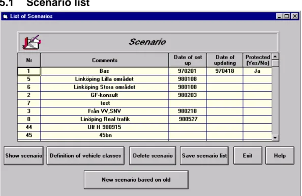
Fig. 5.1 Scenario list, a summary of all created scenarios.
The window in Fig. 5.1 shows the existing scenarios and the facilities available for creating new scenarios. This window is accessed from the function Files at the top of the start window (=cover window).
The program always includes a Scenario No 1 in the form of a file per file type. To create new scenarios, there are two options:
• Copy old to new:
− based on an old scenario
− based on a new composition of old files • "All" new.
To copy old to new:
• Based on an old scenario; see Subsection 5.1.3. This may for instance be equivalent to creating a new scenario with e.g. Scenario No 1 as the basis. Obviously, other scenarios can also be used as the basis.
• Based on a new composition of old files. Enter the window Files included in
scenario and create a new scenario from old files. This window is accessed by
clicking the button Show scenario.
All new: Enter the number, comments etc in the scenario list and save the scenario list. Give a new definition of Vehicle Level 2; see Subsection 5.1.2. A new file per file type must then be specified.
The user may make every created scenario a read-only file.
If the user wants to see what files are included in a scenario, he/she selects the number concerned in the list and clicks the button Show scenario. This brings up the window Files included in the scenario.
When the pointer is placed on a certain scenario and the button Remove
scenario is clicked, the scenario definition is removed. All files which are unique
to this scenario are also removed. Files common to several scenarios are not affected but remain.
If there is something new in the scenario list, the button Save scenario list must always be clicked before leaving the window.
Examples of possible scenarios might be: • national base scenario
• regional base scenarios
• different rates of economic growth • increase in public transport
• increased road investment
• large scale investment in alternative fuels • faster scrapping of old vehicles.
5.1.1 Files included in the scenario
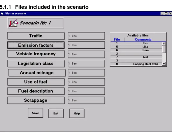
Fig. 5.2 Files included in the scenario.
In Fig. 5.2, the window Files included in the scenario shows what files are included in a scenario. This window is accessed via the window Scenario list and the function Show scenario.
By clicking on the file type concerned, the available files per type can be seen. This shows both what file is included in the scenario concerned and all files that are available for creating new scenarios.
Since the same file content may be assigned to many different file numbers, it would be advisable to append explanatory comments to every file.
if an impermissible file combination is selected. If the requirement is not satisfied, an error occurs when an attempt is made to perform a calculation.3
Two file types are independent of Vehicle Level 2, i.e. they can be combined with all other files: traffic data and fuel description. These two are given at Vehicle Level 1. Other file types are given at Vehicle Level 2.
The number of the scenario to which the window refers is shown in the top left corner of the window. There is one window per scenario of this type.
5.1.2 Vehicle definition
Fig. 5.3 Vehicle definition, i.e. definition of Vehicle Level 2, is a subdivision of the fixed vehicle types (Level 1).
The window Vehicle Definition in Fig. 5.3 is accessed via the window Scenario
list and the function Define vehicle. Vehicle types are defined at two levels, 1 and
2. Level 1 is fixed and comprises the following:4
No
3 The program should in actual fact state for each file which Vehicle Level 2 the file refers to. At
present the only way this is made evident is that the calculations may be unsuccessful. The user must for the present keep a check on what files are included in a certain Vehicle Level 2. It is naturally the easiest to keep to one definition throughout.
4
In the base file attached to EMV it has been decided to use those definitions of vehicle types, at Level 1, which are included in the Road Traffic Proclamation.
• car (1) • light truck (2) • truck (3.5) - 16 tonnes (4) • truck 16 - tonnes (5) • bus (3) • moped (6) • motorcycle (7) This numbering shall always be used at Level 1.
Level 2 provides an opportunity for subdivision per vehicle type within Level 1. The example in Fig. 5.3 shows a subdivision of light trucks into three groups.
Note that, for each scenario, the user must give definitions for Level 2 even if these are identical with Level 1. The number of the scenario is shown in the window.
If the user wishes to work with a finer structure than Level 1, this can be created at Level 2. In the base scenario both light truck and bus have been subdivided into three subgroups at Level 2. It may also be appropriate to subdivide cars into different weight classes.
At Level 1 work is based on number per type, while at Level 2 it is based on optional alphanumeric name.
Working with different parallel definitions at Vehicle Level 2 reduces the possibility of combining different files into new scenarios.
When a definition is to be made, the alphanumeric name is entered in the field after Vehicle level 2 - name. After this the definition at Level 2 shall be coupled to Level 1 in Which new Vehicle Level 2 is included in Vehicle Level 1. When this text or the field where the information is to be entered is selected, a table is displayed with all available options at Level 1. The option in question is then selected in the table.
In Fig. 5.4, the window New scenario is used to create a new scenario on the basis of an old one. This window is accessed from the window Scenario list and through the function Create new scenario from an old one. Select the scenario number which is to be the base scenario. Enter the new scenario number, scenario name and the date of creation. Click OK. Scenario created comes up. All the files needed in the new scenario are created automatically with the same file number as that of the scenario. Note that the specified sequence of operations must be followed. The data files in the new scenario can now be altered as wished.
6 Data
files
The following window types are found under this heading: • File type
• File list • File content • Item description
For some file types, the item description can be given as both a Window A and a Window B.
Window B is an expansion of the first window, i.e. Window A.
To create a new file, with the exception of Traffic data and Fuel description, it is necessary first to define Vehicle Level 2 and also a scenario5. New files can be created as follows:
• by creating a new scenario
• by directly entering a new file in the file list.
The data files which constitute a scenario should relate to the same geographical region.
Each file has an upper limit for the maximum number of items. The only case we know of where this may be a practical problem is for Use of fuel; see also Subsection 6.4.6.
6.1 File
types
Fig. 6.1 File types, the screen from which the desired file type can be accessed.
The window in Fig. 6.1 is accessed via the function Files/Data files at the top of the start window (= cover window).
There are eight file types to choose from: • Traffic files
• Vehicle description • Vehicle frequency
• Division into legislation classes • Annual mileage
• Use of fuel • Fuel description • Scrapping
File type: Clicking one of the eight text boxes brings up the file list for the file
6.2 File
list
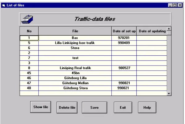
Fig. 6.2 Example of a file list. There is one file list per type of file.
The window File list in Fig. 6.2 is accessed via File types.
For each file type there is a file list. Each file must have a unique number in the list.
The same file content may occur under different file numbers.
To view or update a file, select this file. The file is shown by double clicking
No or clicking the button Show file after selecting the required No.
When a new file is created, it shall be given a new unique file number and a comment, i.e. unless the new file is created through Scenario list. It may be advisable to fill in the date when the file is created and the date when it is updated. Files can be made read-only through Scenario list. This is only evident from Scenario list.
No: Each new file has a unique number within the file type. File: The user should enter a key word which identifies each file. Date created: Given manually.
Date updated: Given manually.
Show file: Means that the selected file, an item overview, comes up. Remove file: See command buttons, Section 4.
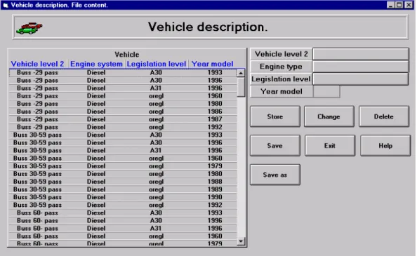
6.3 File content
An example of File content is given in the window in Fig. 6.3.
Fig. 6.3 Example of window type File content.
The window File content in Fig. 6.3 is normally accessed from File list.
All file types with the exception of Traffic Data have a window with file content, i.e. the items included in the file. Traffic Data is accessed directly from the file list for the data items. The groups to which other file types can be assigned are vehicle oriented file types and others. Others consist only of the file types Fuel Description. As regards the vehicle oriented file types, Vehicle Level 2 is generally used as the basis of classification.
All items included in the file are listed in a table at the left of the window. The right side contains tools for changing the file content. The item identification is given at top right of the window.
The buttons in the window have the following functions: • Add item can be used
− to add a completely new item − to copy an old item
• Change item
− some part of the item identification has been changed
• Remove item, select in the table the item concerned and click the button. To add an item, select this button. At bottom right of the window a table is displayed showing the available options for Vehicle Level 2. Select one of these. Enter the information concerned.
Save as is used to create a new file on the basis of an old one. At this stage a
file has already been chosen, and this can be saved in the file list under a new number. The old file remains parallel with the new one.
Before the window is closed after making the changes, the button Save must first be clicked if the information entered is to be retained.
6.4 Item
description
Examples of item descriptions are given in Subsections 6.4.1 - 6.4.8.
In order to access the level Item Description, select the item concerned in the appropriate window of File content.
The identification of the item description is displayed at the top of the window. This identification cannot be altered from this window. All other data in the window can be altered.
In order to enter new data or change old data, enter the new data in the appropriate field. Click the button Store, except in the case of Traffic data where the alternative is Save. The reason for this apparent lack of consistency is that the traffic data window is at the same level in the data structure as File content.
In cases where there is both a Window A and a Window B, this is shown by the addition of the letter A or B to the window heading. In such cases " … B" is displayed directly below the line containing the window heading. By selecting this field, Window B is accessed. The purpose of having a Window A and a Window B per item is to provide space for more information than can be accommodated in only one window.
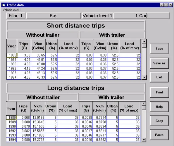
6.4.1 Traffic data
For Traffic data, the window in Fig. 6.4 is a combination of File content and
Item description.
The user decides which geographical region the traffic data refer to. Examples of regions may be: national level; a county; a municipality, etc.
Calculations can be performed from the first up to the last year with traffic data. Data need not be given for all the years between the first and last in a series. Calculations can nevertheless be performed for such intermediate years by interpolation.
Data should be given at least for years that represent a change in development, even though this is not a requirement.
Each window refers to a vehicle type defined as Vehicle Level 1. Vehicle Type 1 is shown at the top left corner of the window. Clicking this field brings up a table with the available Vehicle Type 1 options. Selecting a certain Vehicle Type 1 displays the requested item with traffic data. Vehicle type 'car' is the default.
Short/long distance trips: The dividing line between short and long distance
trips is normally 100 km. This boundary is optional. The reason for the division is that the following data depend on this variable: proportion of travel with a trailer; load, and travel in urban area. It may in addition be of great interest to have output data broken down into short and long distance trips6. It is also conceivable that different subdivisions into vehicle type may depend on length of trip.
With or without trailer: According to the model, all vehicle types can to some
extent be driven either with or without a trailer.
Year: The year to which the traffic data relate. Data need not be given for all
years. The same year must be given for both short and long distance trips.
Number of trips (Giga No)7: Number of trips or starts per year. There is a
coupling here to the correction factors for cold start. What is important is that the same definition of trip and also start should be used for both the correction factors (cold start) and trips in Traffic data. What should be used is a trip definition which has the effect that the number of trips is equal to the number of engine starts.
Fkm (Gfkm): Annual mileage for the vehicle type concerned (Level 1).
Urban area (%): Percentage of mileage in an urban area. The definition of urban
area for traffic data shall be the same as the urban area description to which the emission factors for urban area in the vehicle description relate. The urban area definition chosen is a matter for the user. A suitable definition may be the one used by Statistics Sweden. This should also be appropriate if the costs of exhaust emissions shall be estimated. This would give different values for rural and urban areas. In turn, this is equal to a distribution on the basis of whether or not people are exposed to the emissions.
Load (% of max): Average percentage utilisation of maximum load (weight) or
maximum number of travellers. This affects the resulting emission factors through Window B in the vehicle description.
6 Such an output data facility has not yet been implemented.
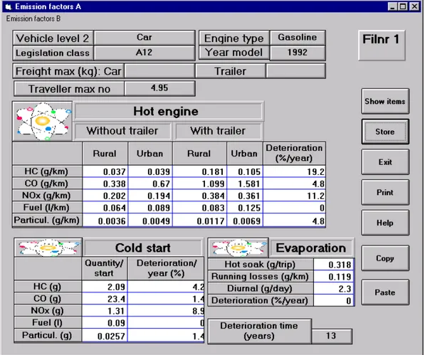
6.4.2 Vehicle description
Vehicle description A
Fig. 6.5 Vehicle description A with emission and fuel factors.
In the window in Fig. 6.5, Vehicle description A describes all fuel and exhaust factors, i.e. the quantity of fuel or exhaust emission per unit of distance driven, per engine start or per unit time while parking. The item type comprises both a Window A and B. Window B is accessed by selecting Vehicle description B at top left.
One requirement is that there is at least one window per Vehicle level 2,
Engine type and Legislation class. If there are changes at year model level
within such a group, such a development can be described, i.e. with several windows per combination in accordance with the last sentence.
The values of the factors given shall agree with the specified load in the window Relationship between emission factors and load (B).
If load is changed in traffic data, the resulting emission factors for hot emissions are automatically adjusted with correction data, according to Window B, if such data exist.
The values of factors in Vehicle description are dependent on the correction factors according to Chapter 7 and on the definitions chosen for traffic data according to Subsection 6.4.1.
Fuel consumption is given in litres/km, which also holds for gas driven vehicles.8
The use of factor values in the program is normally self evident, i.e. distance specific values are multiplied by vehicle mileage, and start specific values by the number of starts. One exception is evaporation of the diurnal type. The value of the factor refers to emission per 24 hours, in which way an hour specific value can be calculated. The number of parking hours is estimated by assuming an annual mileage of 15,000 km at a speed of 60 km/h. The number of hours driven is subtracted from the number of hours per year, which gives the hours of parking. Finally, the parking time in combination with the diurnal value per hour gives a diurnal value and an annual value.
Vehicle level 2: Follows automatically from the description given under File
Content.
Engine type: Follows automatically from the description given under File
Content.
Legislation class: Follows automatically from the description given under File
Content.
Year model: Follows automatically from the description given under File
Content. If several year models are described per legislation class, interpolation will be performed for any intermediate years without input data in the form of vehicle description.
If a description is given for only one year model per legislation class and this legislation class comprises several year models, the data specified must hold for all year models within the legislation class.
Freight max (kg): Given for both vehicle and trailer. Can be used to relate
emissions to tonne mileage. No such function has been installed for the present. There is therefore no requirement to supply data.
Travellers max number: For cars includes driver and for buses excludes driver.
Same as for the previous item.
Hot emissions (g or l/km): Level representing a new vehicle. For the different
combinations of with or without trailer, rural or urban area, levels are given representing a new vehicle exclusive of cold start effects. The values supplied shall represent an load according to Window B.
Deterioration, hot emissions (%/year): The value supplied shall be related to
the hot phase of a new vehicle. Only one common value for urban and rural areas can be given here.
8 The densities of the fuels to which the vehicle description refers are assumed to be as follows:
- gasoline: 0.755 kg/dm3
- diesel: 0.840 kg/dm3
- alcohol: 1.0 kg/dm3 (fictitious)
- gas: 1.0 kg/dm3 (fictitious)
For fuel mixtures there must be separate emission factor windows for the constituent fuels. The resulting emission factors are based on the proportions of the different fuels. This has not been implemented.
Cold start (g or l/start): A level relating to a new vehicle at 20°C shall be given.
If the increase is based on FTP75, the estimate that is sought is as follows:
(Bag 1) - (Bag 3 with reduction for 10 minutes' stop). If another definition is chosen, the correction file for the cold start must also be updated.9
Deterioration, cold start (%/year): The value given shall be related to the cold
start for a new vehicle.
Evaporation. Level representing a new vehicle. The different parts refer to the
following:
• Hot soak (g/trip), the increase in emission which occurs directly after parking due to the fuel having been warmed up.
• Running losses (g/km), the evaporation which occurs while the vehicle is in motion.
• Diurnal (g/24 hours), the evaporation from a parked vehicle as a results of temperature alternations.
Deterioration, evaporation (%/year): The value given shall be related to all
evaporation from a new vehicle.
Deterioration time (number of years): All emission factors are changed by the
stated deterioration per year up to the specified number of years. The emission level after this is unchanged.10
9 The cold start values in the enclosed base file represent the test cycle for cold transient Yct and hot transient
Yht in FTP75. According to (Sérié and Joumard, 1996) the cold start is a function of the test cycle, i.e. it is probably insufficient to use a general set of cold starts. By using the correction factors for cold start, see Section 7.2, it is possible to deviate from the base values. One can obviously choose one's own values and enter these directly into Vehicle description, but these must always be suited to the correction factors.
10 Is it realistic to assume the same number of years of deterioration for all phases and substances? In the
Vehicle description B
Fig. 6.6 Vehicle description B with correction factors for load conditions different from those to which Vehicle description A refers.
In the window in Fig. 6.6, Vehicle description B describes the relationship between emission factors for hot emissions and load.11
There is one Window B per Window A.
There shall be separate corrections for four situations per substance.
Base level A refers to load (%): Refers to the load level (weight or number) to
which the factor values in Window A refer.
Correction (% effect/% load deviation): If the value given in a certain cell is P,
the resulting load corrected emission factor is:
{[(Load according to Traffic) – (Base level load)] × P/100+1} × (Base factor according to Window A).
11 Is it realistic to correct only hot emissions? In the same way as the cold start is a function of the test cycle, it
6.4.3 Vehicle frequency
Fig. 6.7 Vehicle Frequency per Vehicle Level 2 and year, and distribution by Engine type.
In the window in Fig. 6.7, Vehicle frequency forms the basis for a distribution of traffic data by Year model and Engine type.
There shall be windows for at least 2 years per Vehicle level 2.
This gives a description per year of the vehicle frequency per year model and the distribution by engine type (engine type).
Vehicle level 2: Follows automatically from the description given under File content.
Year: Follows automatically from the description given under File content. Year model class: A total of 20 classes. The first 19 classes are specific year
models, and the last one is an amalgamation of year models from the 20th onwards. The first class, for instance, for 31/12 of year 1996 is year model 97.
Vehicle frequency: The number per year model on 31/12 of the year given for the
area the traffic data refer to. The time given is significant since the program describes the effect due to the fact that the vehicle frequency per year model changes during the year. This may be of particularly great importance for the first two (=youngest) year model classes when these are to be assigned an annual vehicle mileage. Summation of Vehicle frequency over all year model classes produces what in the following is referred to as total number. For years where no
• if calculation year is earlier or the same as the first year with numbers:
− estimates total number on the basis of traffic data and the first year with numbers
− estimates distribution by year model on the basis of probability of scrapping • if calculation year is between two years with numbers:
− total number is calculated by interpolation between latest previous year and earliest subsequent year with numerical data
− number of year models is calculated in two ways:
− by interpolation between the numbers of the year model concerned for the two years with numbers
− by using probabilities of scrapping if interpolation cannot be performed • if the calculation year is later than the latest year with numbers:
− total number is estimated on the basis of traffic development
− number of year models for old year models, Year model class 3 and later, is estimated on the basis of probability of scrapping and the latest year with numbers
− the number of new vehicles in the first two year model classes is formed as the difference between the total number and the sum of the number of year models according to the previous indent.
− The number per year model of the first two classes shall be larger than a reasonable minimum level. If this is not satisfied, corrections are made; see also Subsection 9.2.2.
The term total number refers to the sum of all year models at a certain Vehicle
level 2. In some cases as above, this total number is assumed to be altered in
direct proportion to the change in traffic data at Vehicle level 1. What should in actual fact have been used are traffic data corresponding to Vehicle level 2. Since these are not available, Vehicle level 1 is used instead.
Engine type (%): The term engine type refers to gasoline, diesel, alcohol and
gas. The distribution per year model shall refer to 31/12 in the given year. Each row must add up to 100%.
If calculations are to be made for years without "Number", distribution of the model by engine type is described as follows:
• data are available only for later years:
− if the year model is not specified for later years, choose the distribution according to the twentieth year model class for the first subsequent year with data
− if the year model is given for later years, choose the distribution for the first year with such data
• data are available only for earlier years:
− if the year model is not given for earlier years, choose the distribution for the latest specified year model
− if the year model is given earlier, choose the distribution for the year model that was specified with the latest year with numerical data
• data are available for both earlier and later years:
− year model concerned is given both earlier and later: interpolate between these years
− year model concerned is given earlier but not later: interpolate between the previous distribution and the twentieth class for later years
− year model concerned is given for later but not for earlier: interpolate between the youngest earlier year model and the first later year for which input data are available for the year model concerned.
6.4.4 Distribution by legislation class
Fig. 6.8 Distribution by Legislation Class per Vehicle Level 2, Engine type and Year Model
In the window in Fig. 6.8, Distribution by legislation class is the basis for the distribution of traffic data by legislation class.
There shall be a window per Vehicle level 2 and Engine type.
It is assumed that distribution per individual year model is independent of year. Data need not be given for each year model, with the exception of those for which a new legislation class is introduced. The table can be extended, i.e. there is an "unlimited" number of rows.
Vehicle level 2: Follows automatically from the description given under File content.
Engine type: Follows automatically from the description given under File content.
Year model: All year models with new legislation classes shall be specified
Legislation code: The code may for instance be A10. The same code must appear
in vehicle description and use of fuel.
Distribution (%legislation class): The user can give only one distribution per
year model, i.e. distribution is assumed constant in time per year model. This solution will result in a deviation from reality. In reality, distribution for one and the same year model may vary from year to year.
Each row must add up to 100%.
If calculations are to be performed for years with year models which are not included in Distribution by legislation class, the legislation class distribution for the oldest or youngest year model in Distribution by legislation class is to be used.
The distribution entered most recently is assumed to hold for all subsequent year models. If the legislation class distribution has been specified for year models n and n+2, year model n+1 will be allocated the same distribution as year model n. Note that no interpolation is performed.
If the user wishes to test his/her own distributions in new scenarios, it is sufficient to enter legislation class distributions; numerical data are not required for the same years. It should for instance be possible to test 100% MK1 from year model 1998 even though the last Numerical data refers to 31.12.1995. There is no requirement to enter data in the numerical window for the same year.
If during the current year the most up-to-date description possible is to be made, this should refer to 31.12 the previous year. The last (=youngest) year model would be that of the current year. Since at this time the year model for the current year has not all been sold, there is a great risk that the distribution by legislation classes for this year model will in time change more than marginally. When the file is supplemented with new year models, it should at least be reasonable to update the three year models which have been entered most recently. Explanation: if the year model entered most recently is the model of year 1996 and at the time of the next updating data are available up to year model 1997, then 1994, 1995 and 1996 would also have to be updated since sales of all these year models may be expected to continue during year 1996. What should be the procedure when the distributions for older year models are changed in time in a more general manner? One alternative could be to create different scenarios, with one scenario for instance having the distribution for 31.12.1993 and another the distribution for 31.12.1995. If calculations are to be made for the emissions in year 1993, the scenario with the distribution from 31.12.1993 is chosen, and so on.
6.4.5 Annual mileage12
Fig. 6.9 Annual mileage (A) per year, Vehicle Level 2 and Engine type
In the window in Fig. 6.9, Annual mileage forms the basis for the distribution of traffic data per Vehicle level 2, Engine type and Year model.
Annual mileage as a function of age is described per Vehicle level 2, Engine
type and Year.
A minimum requirement is that there should be at least one window per
Vehicle level 2 and Engine type.
For the previous and subsequent year, see Vehicle frequency, the program chooses the first and last description respectively in the input data for Annual
mileage.
Year: Follows automatically from the description given under File content. Vehicle level 2: Follows automatically from the description given under File content.
Engine type: Follows automatically from the description given under File content.
Age class: The class referred to is evident under the heading Vkm/year below.
The last class (20) refers to 19 years and over.
Vkm/year: This gives the annual mileage for the time or age interval. The
structure of the program is such that the mileage given is that expected during a year for a vehicle at the beginning of each class, i.e. for the first class the mileage during the following year for a completely new vehicle. For the last class, the annual mileage chosen is that representative for all vehicles which are at least 19 years old.
6.4.6 Use of fuel
The aim of this file type is to describe how different combinations of Vehicle
level 2 and Engine type use different fuel types and fuel qualities according to the
description of fuels in Subsection 6.4.7. Owing to the greater incidence of mixed fuel vehicles, different fuel types may occur per engine type. For instance a mixture of gasoline and alcohol may be described. Different distributions may be described for different legislation classes.
The base file does not include the mixed fuel alternative, but only that a certain combination of Vehicle level 2, Engine type and Legislation class can drive on different fuel qualities.
Use of fuel and Fuel Description have a strong coupling with Correction for Fuel quality.
The window is used to distribute traffic data on the basis of the use of different fuel qualities. The item type comprises both a window/form A, Fig. 6.10, and B, Fig. 6.11.
There shall be at least one window per Vehicle level 2 and Engine type.
Every introduction of a new fuel or fuel quality for the group of vehicles demands a new pair of windows (A and B).
Use of fuel Form A.
Fig. 6.10 Use of fuel (A) per year, Vehicle Level 2 and Engine type.
In the window in Fig. 6.10, Use of fuel Form A describes the percentage driven with different Fuels per Legislation class/Group code.
The fuel codes (1-12) are the same as in the definition of the mixed fuel group and in the fuel description; see Window B.
Note that, for instance, fuel code (3) need not correspond to fuel in Exposure Class 3 but forms part of a consecutive code for all the described fuels. Fuel Code (3) may also mean different fuel descriptions for different years. What is important is that the definitions in Use of Fuel and Fuel Description agree.
What must be entered into the columns in the window is the percentage driven with different fuels per legislation class. Data on how fuel supplies are broken down per different types and qualities can be obtained most easily from the fuel suppliers. Note that this is not exactly what is sought. In the absence of better data, however, the distributions must be based on supplies. In the program the emission factors for fuels are weighted according to the distribution entered.
The percentage driven per fuel type is to be given in each cell. Each column with values must add up to 100%.
Legislation class/Group code: According to Use of fuel in window/form B. The
object of forming groups of legislation classes is to reduce the space problem. The alternative would be a table with the same number of columns as the number of legislation classes during the calculation year.
Gasoline (1-4): Quality in accordance with the fuel description. Diesel (5-8): Quality in accordance with the fuel description.
Alcohols F (9-10): Quality in accordance with the fuel description. F = fossil. Alcohols B (11-12): Quality in accordance with the fuel description. B = biomass. Gas F (1-2): Quality in accordance with the fuel description. F = fossil.
Gas B (3-4): Quality in accordance with the fuel description. B = biomass.
Mixed fuel: Composition in accordance with Use of fuel Window/Form B. The
mixed fuel group is used for vehicles driving on mixed fuels (see Window/Form B). If the use of mixed fuel is specified, the emission factors for each fuel type must be described under Vehicle description.
Use of fuel, Form B
Fig. 6.11 Use of Fuel (B) per year, Vehicle Level 2 and Engine type. Definition of legislation class groups. Groups of legislation classes and of mixed fuels can be defined here.
In the window in Fig. 6.11, Use of fuel Form B defines legislation class groups and mixed fuels.
Legislation class/group code: Legislation classes can be put into four groups per
Since the number of legislation classes changes in time, different legislation class groups may be formed in different years. In the base file, "all" is used as a general designation since no fuel quality has any special effect on the fuel and emissions factors. The only effect on emission factors that is described in the base file is via the aromatic compounds content of diesel. The relative effect is however the same for all legislation classes, i.e. in this case also all is sufficient.
Fuel code/Mixed fuel group.13 The function is not implemented.
6.4.7 Fuel description
Fuel description A
Fig. 6.12 Fuel Description (A) per year and the appropriate fuel types and qualities.
The window in Fig. 6.12 is used as the basis for the correction of emission factors in the light of the fuel content in question. As regards Sulphur and Lead, these can be used directly in combination with fuel factors in calculating emissions of SO2 and Pb. By combining the data in Fuel description with data in Correction
for fuel quality, Fig. 7.3, it is possible to influence the fuel and exhaust factors
and thus the resulting emissions. The fuel codes are the same as for use of fuel. The item type comprises both a Window A and a Window B.
The symbol (w) denotes percentage by weight and (v) percentage by volume. One row in the table represents one fuel quality.
There shall be one window for every year when there has been a change. Data need only be entered for the fuel that has been changed. There shall be at least one window.
13 This states whether there are vehicle groups using mixed fuels.
The substances which, according to the base file, have significance for the results are aromatic compounds, sulphur and lead. The user can alter this by creating a new scenario with alternative correction factors for fuel quality; see also Section 7.3.
Fuel description B
Fig. 6.13 Fuel description (B) per year with miscellaneous data per fuel type and grade.
In the window in Fig. 6.13, Fuel description B refers to miscellaneous data. For each Window A there shall be a Window B.
For the present only the density of the fuel is obligatory. What is affected in the output data is use of fuel. This effect is described by assuming that use of fuel in
Vehicle description has fixed densities as follows:
• gasoline, 0.755 kg/dm3 • diesel, 0.840 kg/dm3 • alcohol, 1.0 kg/dm3 (fictitious) • gas, 1.0 kg/dm3 (fictitious)
• energy content - to have a measure of general applicability for comparisons both between vehicles with different engine types within the road traffic sector and between vehicles within the road traffic sector and other sectors
• vapour pressure - to improve the description of evaporation
• price - the ability to describe the personal economic or macroeconomic costs of the fuels used
• environmental costs - the ability to state the total emission costs as output data. Subdivision is needed into rural and urban areas
• the total costs for road traffic due to taxes and charges on fuel.
6.4.8 Scrapping
Fig. 6.14 Probability of scrapping per age class and year.
The window in Fig. 6.14 forms the basis for the numerical description per year model in certain cases where these were not entered as input data; see the description below. There shall be at least one window per Vehicle Level 2.
For years before the first year with available numerical description, the probability of scrapping is used in general in determining the number per year model class.
For intermediate years, i.e. where the number per year model is given both before and after the calculation year, interpolation is performed where possible. In other cases, i.e. where the number for a year model is given for only one adjacent year, the probability of scrapping is used for the description of the intermediate
For the prediction year, the year after the last year with numerical description, scrapping in general is used in describing the number per year model.
In the base file, the latest window for the vehicle frequency and cars refers to the year 1995. If a calculation shall be made for 1996, the number per year model on 31.12.1996 must be estimated. This is to be based on numerical data for 31.12.1995 and the probability of scrapping for the latest year. The vehicle frequency of e.g. year model 1991 in 1996 is estimated by using the number for 1995 and the probability of scrapping in the sixth element in Scrapping.
Year: To which the distribution refers (31.12). Vehicle level 2: As before.
Age (year): Year model class, i.e. the same classes as in Vehicle frequency. Probability of scrapping (%): Probability of scrapping within the j:th year
model class when the age increases by one year. In the model no vehicles are scrapped in the first three years. In the window, the column heading "Age (year)" is used rather erroneously instead of year model class, the alternative which shall be used. In most cases, however, the difference is small. If the number of years were to be retained, the first column would instead read as follows: 0.25 (1); 0.75 (1); 1.75 (2), and so on.
7 Correction
files
For correction with respect to humidity, cold starts and fuel quality, there are special correction files. These files are accessed via the top edge of the start window.
For cold starts and fuel quality, there is a file list in the same way as under files.14 The number of items in these two file types is given by the contents of
Definition of vehicle level 2, Vehicle frequency and Distribution by legislation class.
Throughout, blank is interpreted as 1 in the correction files.
7.1 Correction for humidity
Fig. 7.1 Correction for humidity for NOx
When NOx is measured in the laboratory, a correction is normally made with
respect to a reference situation. The aim of the EMV model is to describe exhaust emissions on Swedish roads for representative temperatures and humidities. Laboratory data must therefore be corrected from the reference situation to normal Swedish conditions. If a certain correction is for instance entered for gasoline, all NOx emitted from gasoline engines will be generally corrected with the specified
value.
This file type has no coupling at present with scenario. It is therefore not possible to have different values for different scenarios, i.e. the same corrections hold for all scenarios.
The factor by which the NOx factors must be multiplied is given in Fig. 7.1 for
each fuel type.
Gasoline: correction factor. Diesel: correction factor. Alcohol: correction factor. Gas: correction factor.
7.2 Correction for cold start
Fig. 7.2 Correction for cold start per Vehicle Level, Engine type, Legislation class and Substance.
Cold starts measured in a laboratory environment normally refer to a start temperature of ca 20°C. The cold start in the vehicle description also refers to 20°C. Starts in real traffic are made at other engine temperatures as a function of air temperature, parking alternative, use of engine heater, etc.
The influence of these conditions can be described by correcting the cold start; see Fig. 7.2.
The correction shall refer to "increase" (extra amount/start) and nothing else. VTI has a calculation program called COLDSTART which takes account of "all" relevant factors of major significance for the correction. Using this, representative correction factors can be calculated for optional conditions such as: different geographical regions; different starting places; different times during the year; different types of engine heater, and so on.
There is one file per scenario, i.e. the file number and scenario number are always the same.
The actual item identification, i.e. the first three columns, is automatically filled in with data as a function of the items which have been entered in Vehicle
frequency and Legislation class.
Note that the file type is not included in the window Files included in the
scenario.
There are two alternatives for entering data in a new file:
• using Create new scenario from an old one in the scenario list (window) • creating a "completely" new scenario.
In the first case data have been automatically assigned to the correction file. The second alternative implies that a new correction file has been created but it has no contents. Data according to the above description must then be entered in the file
manually. It is not a requirement that COLDSTART is to be used in producing correction factors.
Vehicle level 2: As before. Engine type: As before. Legislation class: As before.
Correction/substance: The value entered is multiplied by the cold start according
to Vehicle Description A. Blank is interpreted as 1. Note that 0 is also interpreted as blank and results in 1. If it is necessary to use 0 as correction factor, the alternative is to use a very small value.
7.3 Correction for fuel quality
Fig. 7.3 Correction of emission factors when the fuel quality used is different from the fuel to which the emission factors refer.
The purpose of the window in Fig. 7.3 is to make it possible for the emission factors for one and the same vehicle to be changed between different years as a result of using a fuel quality different from that referred to in Vehicle
description.
There is a set of data per Vehicle level 2, Engine type and Legislation class. New files are created in the same way as for the correction of cold start. Data have been grouped in:
• Emission factors correspond to • Effect change (%/%).