Feasible customer order decoupling points and associated inventory costs

(1)

Feasible customer order decoupling

points and associated inventory costs

Jesper Madsen

Betim Mavraj

(2)

This exam work has been carried out at the School of Engineering in Jönköping in the subject area operations management and logistics. The work is a part of the Master of Science programme Production Development and Management.

The authors take full responsibility for opinions, conclusions and findings presented.

Examiner: Jenny Bäckstrand

Supervisor: Fredrik Tiedemann & Joakim Wikner Scope: 30 credits (second cycle)

(3)

Abstract

Purpose - The purpose of the thesis is to develop a method that simplifies the analysis between reduction of delivery lead time and inventory costs, when the reduction of delivery lead time is achieved through repositioning of the customer order decoupling point.

Research questions - The purpose of the research has been broken down into three research questions. By answering these three questions the authors believe that there is enough information gathered to reach the purpose (i.e. develop and present the desired method). The following three research questions were posed:

RQ1: What determines a products delivery lead time?

RQ2: How are feasible customer order decoupling points identified? RQ3: How are inventory costs affected by the positioning of the customer order decoupling point?

Method - The research have followed an abductive approach, i.e. the authors have switched between empirical investigations and theory building through literature reviews. In practice, to build theory, both case study research and analytical conceptual research were iterated throughout the research. Literature reviews, document sampling, interviews, and observations have been used to collect data.

Findings and conclusion – A method, referred to as the DC-method, have been developed. In a total of 9 steps, the DC-method guides stakeholders through the identification of feasible customer order decoupling points, factors to consider when analyzing feasible customer order decoupling points, and lastly presents how changes affect inventory costs.

(4)

Figures

FIGURE 2.1.RESEARCH PROCESS. ... 6

FIGURE 2.2.RESEARCH APPROACH. ... 7

FIGURE 2.3.STRUCTURE ON THE CONDUCTED INTERVIEWS. ... 11

FIGURE 2.4.ANALYSIS OF DATA... 14

FIGURE 3.1.ILLUSTRATION OF THE THEORETICAL BACKGROUND. ... 18

FIGURE 3.2.PRODUCT STRUCTURE OF THE END PRODUCT P ... 20

FIGURE 3.3.VAX MATERIAL PROFILES ... 20

FIGURE 3.4.TIME-PHASED PRODUCT STRUCTURE FOR THE END PRODUCT P ... 22

FIGURE 3.5.CONCEPT OF THE S:D RATIO ILLUSTRATED WITH THE CODP. ... 23

FIGURE 3.6.FEASIBLE TIME-PHASED POSITIONS OF THE CODP ... 26

FIGURE 3.7.THEORETICAL FRAMEWORK. ... 31

FIGURE 4.1.PRODUCT STRUCTURE OF PRODUCT 1... 34

FIGURE 5.1.TIME-PHASED PRODUCT STRUCTURE AND CURRENT CODP. ... 41

FIGURE 5.2.ILLUSTRATIONS OF FEASIBLE CODPS IN PRODUCT 1'S TIME-PHASED PRODUCT STRUCTURE. ... 43

Tables

TABLE 2.1.SEARCH TERMS. ... 10

TABLE 2.2.INTERVIEWED KEY PERSONNEL. ... 12

TABLE 3.1.INDENTED BOM ON PRODUCT STRUCTURE IN FIGURE 3.2. ... 21

TABLE 3.2.SERVICE LEVEL AND SAFETY FACTOR. ... 29

TABLE 4.1.INDENTED BOM OF PRODUCT 1. ... 36

TABLE 4.2.YEARLY DEMAND AND VALUE IN SEK FOR RELEVANT ITEMS IN PRODUCT 1. ... 37

(6)

(7)

1 Introduction

This introducing chapter will give an overview of the background, including the arguments and reasons to why the chosen topic is of importance. Moreover, the problem description is formulated. The purpose and research questions are then presented followed by the delimitations and the disposition of the thesis.

1.1 Background

With an increased and globalized marketplace, local companies are suffering from greater competition from both domestic and foreign actors. With globalization and pressure from customers for faster deliveries, lower prices, and higher variability in choice of products (Reinartz & Ulaga, 2008), it is expected that manufacturing companies strive for a more efficient production. This is usually reached by a streamlined production (Sobek, Liker, & Ward, 1998; Liker, 2004), reduction of waste within the company (Liker, 2004), and cooperation with outside actors, primarily suppliers (Gattorna & Walters, 1996). In general, the aim is to reduce what each product costs to make, and thereby enable a more attractive offer to potential customers.

There is, however, often a tradeoff being made between cost and other performance objectives when efficiency is strived for (Freiheit, et al., 2007; Pundoor & Chen, 2005; Slack & Lewis, 2011). Needless to say is that it is very difficult to reach high quality, speed, dependability, and flexibility while at the same time having low costs (Slack & Lewis, 2011). However, with activities primarily focused on lowering costs, companies risk to overlook potential possibilities to increase revenue. The focus should thus not be towards lowering costs, per se, but towards manufacturing strategies and methods that will result in the highest possible surplus, regardless if this is met by an increase in revenue or through reduction of costs. It is therefore not uncommon that new investments are needed in order to enhance current performance objectives that result in a higher surplus. Nevertheless, companies have trouble to analyze these investments and motivate further improvements. Multiple theories (Ask & Ax, 1997; Begg & Ward, 2009) describe how payback is calculated when investments are made in order to increase output in production. There is however a gap in the theory regarding simple methods for evaluating the value of speed. Some scholars

(8)

al., 2014) have emphasized the importance of valuing lead time. Therefore, the focus in this research will solely be put towards analyzing the performance objectives of cost and speed (i.e. delivery lead time), and the development of methods that simplifies this type of analysis.

1.2 Problem description

Since the focus of the thesis will be towards the performance objectives speed and cost, or more specifically, the cost of reducing delivery lead time, it is interesting to look deeper into the reasons for a reduction in delivery lead time and the importance of cost in this context.

For a reduction of delivery lead time to be valuable, the demand lead time needs to be shorter than the existing delivery lead time (Mather, 1984). Looking at APICS‟s (2005, p.29) definition, this becomes obvious. The delivery lead time is defined as the time from the receipt of a customer order to the delivery of the product and the demand lead time is the amount of time potential customers are willing to wait for the delivery of the product. If the customers are not willing to wait as long as the offered delivery lead time, there is a discrepancy indicating a possibility of increased revenue through the reduction of delivery lead time. When companies strive for reduced delivery lead time, the analysis of the current customer order decoupling points (CODP), i.e. the point for where forecast-driven production turns to customer-order forecast-driven production (Giesberts & van de Tang, 1992), is of relevance. Depending on the choice of strategy for order-fulfillment, the positioning of the CODP and the delivery lead time will vary a lot. Manufacturing companies with a make-to-order (MTO) policy will in general have longer delivery lead times than companies with an assemble-to-order (ATO), or make-to-stock (MTS) strategy. Thus, there is a great chance for MTO companies to reduce their delivery lead time substantially by moving towards an ATO or MTS strategy (Naylor, Naim, & Berry, 1999). However, the practical transition from a MTO to ATO, or MTS strategy is far from simple. Information on how substantial the reduced delivery lead time is, and how much inventory costs are affected, is also difficult to access. Thus, research regarding the reduction of delivery lead time and inventory cost is of great interest.

(9)

1.3 Purpose and research questions

The purpose of the thesis is to develop a method that simplifies the analysis between reduction of delivery lead time and inventory costs, when the reduction of delivery lead time is achieved through repositioning of the customer order decoupling point. More specifically, the method (called the DC-method due to analysis between delivery lead time and cost) will aim to simplify the understanding of lead time for included components and material in a product, and identify how these components and materials affect the overall delivery lead time. The purpose of the research has been broken down into three research questions. By answering these three questions the authors believe that there is enough information gathered to develop and present the DC-method.

RQ1. What determines a product’s delivery lead time?

To effectively reduce the delivery lead time for a product by repositioning of the CODP, it is important to first understand how this lead time is determined. Depending on the products structure different decisions can be taken, or changes be made, in order to reach the purpose of a reduced delivery lead time. However, it is when the fundamentals of the product structure are known that it is possible to effectively reduce the products delivery lead time.

RQ2. How are feasible customer order decoupling points identified? In order to identifying all feasible positions for the CODP, it is required to first understand the basic theory of CODPs. By investigating relevant theory, further knowledge on how to identify the feasible CODP‟s can be obtained. The implication that each feasible CODP will have to the products delivery lead time and the associated inventory costs can then be analyzed.

RQ3. How are inventory costs affected by the position of the customer order decoupling point?

Additionally to the question of “how inventory costs are affected” it is important to know what inventory costs that are affected by the positioning of the CODP as well. Depending on the decided CODP the inventory costs can vary substantially. Hence, there is likely to be differences between a highly forecast-driven flow

(10)

1.4 Delimitations

Since the focus is on the relationship between reduced delivery lead time and inventory costs, there will not be any investigations made towards revenue, even though it is an important aspect to shed light on when defining how big (or small) the costs are. The reduction of delivery lead time itself will be analyzed by repositioning of the CODP. The flow of goods will remain static in the research and no changes to suppliers or the delivery lead time they offer will occur. Due to this, the only inventory costs under investigation are costs for keeping components in inventory (i.e. carrying costs) and ordering costs. No additional costs for transportation or production will be observed. The authors also presume that data regarding carrying cost, ordering cost, and other economic data is available. The DC-method is thus supposed to be of value when this information is known. The authors will neither investigate how to gather logistical data regarding different types of lead time, standard deviation in lead time, etc. This is also presumed to exist before usage of the DC-method. Lastly, since focus in this research is put towards speed, and since speed measures how fast we deliver towards our customers (Slack & Lewis, 2011), the only lead time that will be taken into consideration is the delivery lead time.

(11)

1.5 Disposition

In chapter 1, the introduction to the research is presented. This includes motivation to why this particular topic is of interest. The problem description, purpose and research questions, and delimitations are also stated in the chapter. In order to give a better understanding of how the research has been carried out, the methodology is outlined in chapter 2. The chapter also gives explanation on what data that has been of relevance and how the data have been analyzed. A subchapter with a discussion regarding the validity and reliability of the research ends chapter 2.

All the theories used in the research are presented in the 3rd chapter. Theories regarding mapping of lead time, inventory management, and cost calculations are described and explained throughout the chapter.

The result of the empirical data collected from the case company is outlined in chapter 4. The company, together with data regarding the product under investigation is presented in detail. A supply lead time table summarizes much of the necessary data, such as included components in the product, as well as their respective value and lead time.

The analysis, is based on the theories presented in chapter 3 and the results presented in chapter 4, and is outlined in chapter 5.

In chapter 6, the DC-method with all its 9 steps are presented.

Discussion and conclusions are then presented in the thesis‟s last chapter. Both discussion regarding the methodology and findings is to be found. The research as a whole is further summarized in the end of the chapter, outlining the conclusions that are to be found..

(12)

2 Methodology

This chapter begins with a description of the overall research process and approach applied in the thesis. Further on the theory building methods are elaborated and the data collection techniques are presented. Finally, the indented analysis of data is described and aspects of validity and reliability are discussed.

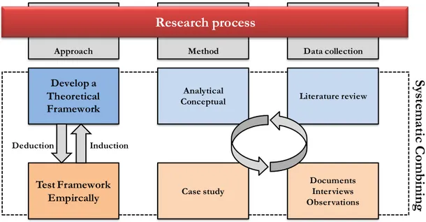
2.1 Research process

The research process illustrated in Figure 2.1 consists of a theoretical part (marked by blue) and an empirical part (marked by orange). In the theoretical part, theory have been collected and developed through literature reviews which then have been tested through a case study. A case study typically uses both qualitative and quantitative research methods for exploring a phenomenon. It can however also be used to develop theory and explain causal relationships (Yin, 1994). In the case study, empirical data was collected through interviews, observations, and collection of documents.

Figure 2.1. Research process.

During the research process the authors have combined theory building and empirical investigations, which can be compared to a shift between induction and deduction (Dubois & Gadde, 2002). Through induction the researchers have encountered and defined relevant variables that later on were reviewed in current literature. The literature reviews generated a theoretical picture of the reality which then was tested empirically, i.e. through deduction. This process has continued throughout the whole research process in order to build and at the same time test the theoretical framework. This approach can be compared to systematic combining, which will be further explained in the following section.

Data collection Method Approach Research process Develop a Theoretical Framework Analytical Conceptual Test Framework

Empircally Case study

Documents Interviews Observations Literature review Deduction Induction Sy st em at ic C om bin in g

(13)

2.2 Research approach

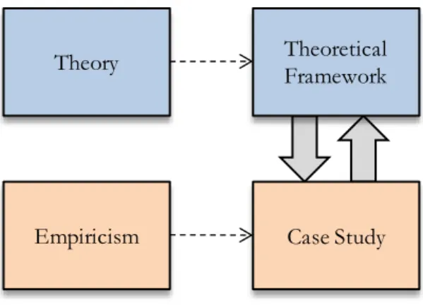
The approach taken in this research can be compared with what Dubois & Gadde (2002) describe as systematic combining. In systematic combining there is a continuous shift between empiricism and theory, enabling the researcher to broaden the understanding of them both. This has had an impact on both the development of the theoretical framework and the empirical investigations. The theoretical framework has been built up over time throughout the research and has been based on empirical discoveries along with input from current theory. The reason for this is simply due to “the fact that theory cannot be understood without empirical observation and vice versa” (Dubois & Gadde, 2002, p. 555). Figure 2.2 shows how the authors have worked with the theoretical framework and the case study in parallel using both theory and empiricism as means to understand the research problem.

Figure 2.2. Research approach.

The systematic combining approach can also be related to the abductive approach described by Spens & Kovács (2006) who discuss the importance of looping theory building and empirical data collection in order to develop new theories. Based on the definitions provided by both Dubois & Gadde (2002) and Spens & Kovács (2006), the approach in this research can be seen as an abductive approach.

2.3 Theory building methods

Wacker (1998) mentions that theory comprises four components: definitions of terms and variables, a specific domain where the theory applies, relationships

Empiricism Theory

Case Study Theoretical Framework

(14)

have been done, which are common ways of doing analytical conceptual and empirical case study research (Wacker, 1998). The theory building methods will be further described next.

2.3.1 Analytical Conceptual

By using analytical conceptual research the authors have linked previously defined theories with each other in order to develop a theoretical framework. This is usually done through deduction (Swamidass, 1986), but in this research a combination of deduction and induction were used (i.e. systematic combining). In analytical conceptual research it is common to build a model of relationships (e.g. a theoretical framework) which later is tested in case studies (Wacker, 1998). However, this has been done in parallel to get a better understanding of the research problem and at the same time to understand which theories that needed to be considered.

Literature reviews have been carried out to collect the necessary data. This is a commonly used method within analytical conceptual research, thus making it appropriate to use in this research as well. A further explanation of the literature reviews is presented in 2.4.1 Literature reviews.

2.3.2 Case study

In order to understand what a case study is, one must first understand what a „case‟ is. A case is an active unit from the empirical world with human interactions (Gillham, 2000) e.g. a single human, a school, or a factory. In order to understand a case it needs to be studied in its context and not as a separate entity (Gillham, 2000). When the above criterion is met, it is possible to perform a case study by looking for evidence in the case setting. This evidence should be collected from different sources (Gillham, 2000) and through different techniques (See 2.4 Data collection).

The case that was put under investigation in this research was Bosch Rexroth, a hydraulic motors manufacturer in Mellansel, Sweden. Their production strategy is MTO or ATO depending on product variant. Bosch Rexroth was selected because they had expressed a need to make informed decisions regarding delivery lead time reductions. It was a two-sided problem where both the actual reduction of delivery lead time and analysis of inventory costs associated with such were troublesome for the company to accomplish. This problem corresponded well with the purpose of this thesis, making Bosch Rexroth a well-suited case company.

When studying only one case, it is referred to as a single-case study (Yin, 1994). Single-case studies allow the researchers to have greater depth in their study, but may reduce the ability to generalize the results (Voss et al., 2002). However, a single-case study was seen as appropriate due to the complexity of the problem. To further justify the use of a case study it should be mentioned that case study

(15)

especially when it comes to theory building (Voss et al., 2002). Furthermore, it can lead to highly practical use in the real world and thus not only contributing to the academic world (Voss et al., 2002).

2.4 Data collection

In order to answer the research questions data has been collected through literature reviews, interviews, document sampling, and observations. In this subchapter we will go through how the data collection techniques were used.

2.4.1 Literature reviews

Literature reviews have been used to collect relevant theory regarding the subject areas in this research. The theory, combined with empirical data, was incorporated into the research process as a means to answer the research questions. Looking at systematic combining, the literature reviews help the authors to find and match theory with the empirical data collected throughout the research (Dubois & Gadde, 2002). A literature review is defined by Fink (2014, p. 3) as:

A research literature review is a systematic, explicit, and reproducible method for identifying, evaluating, and synthesizing the existing body of completed and recorded work produced by researchers, scholars, and practitioners.

As stated by Williamson (2002a), the theoretical framework should be developed based on a literature review. In accordance with this statement, the goal with the literature reviews has been to synthesize existing theories into a theoretical framework (See 3.5 Theoretical framework). With the help of the case study, relevant subject areas could be identified, and literature searches were done in these areas. Due to the multidisciplinary nature of this research, several areas were of interest; logistics as overall (especially delivery lead time), inventory management, and cost. The theories within these areas and their connection to the research questions are further described in chapter 3 Theoretical background. In a literature review one can look in several sources for information. Williamson (2002a) mentions completed research reports, articles, conference papers, books, and theses as potential sources. Fink (2014) talks about bibliographic or article databases as practical sources to find articles, books, and reports in. In addition to this, it may be fruitful to contact experts in the studied area in order to get hold of interesting articles (McManus, et al., 1998).

(16)

In the literature search the authors searched for peer-reviewed articles, books, and conference papers in bibliographic and article databases. The main article databases that have been used are: Emerald, Google Scholar, ScienceDirect, Scopus, Wiley online library, and Primo (Primo is only available at Jönköping University‟s library). Many of these databases have the same articles to some extent. When the same article was found in two different (or more) databases, the authors only included it once. Additional articles were recommended to the authors by a professor of logistics at Jönköping University. After these first steps the authors had collected an initial set of literature. The reference lists in the initially identified literature were then looked through to find more relevant literature.

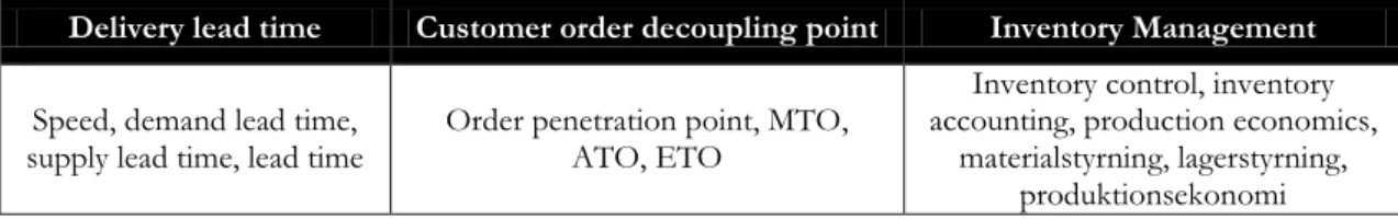
As seen in Table 2.1, the search terms were divided into three groups, delivery lead time, customer order decoupling point, and inventory management. In each group a set of related terms were identified and these words, combined with cost, constituted the complete set of search terms.

Table 2.1. Search terms.

Delivery lead time Customer order decoupling point Inventory Management Speed, demand lead time,

supply lead time, lead time Order penetration point, MTO, ATO, ETO

Inventory control, inventory accounting, production economics,

materialstyrning, lagerstyrning, produktionsekonomi

The only inclusion criteria used in the literature search was that the literature had to be written in English or Swedish. Other than that, the articles were considered appropriate to review. The initial review was made by reading the abstracts and then categorizing the articles as relevant or non-relevant to review further.

2.4.2 Interviews

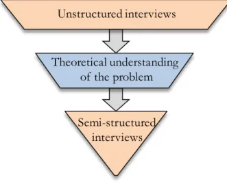
In the early stages of the research, general discussions were held with the supply chain manager at Bosch Rexroth to get insight into how they perceived the problem of making the analysis between reduction of delivery lead time and its impact on inventory carrying costs and ordering costs. The problem was separately discussed with one production manager, the manager of the controlling department, and the sales product manager. These types of discussions can be compared to what Gillham (2002) define as unstructured interviews and were used to get deeper knowledge about the problem. Further on, this made the authors aware of what they had to find out and thus making it possible to ask more focused questions.

After the initial unstructured interviews the authors got a better understanding of the problem at hand, and how it was experienced by the case company. To further build on the knowledge about the problem, searches in literature was done in order to construct a theoretical understanding of the problem. This made it easier to develop more specific questions and select key personnel to interview, also

(17)

referred to as key informants by Voss et al. (2002). Voss et al. (2002) further state: if reliable key informants can be identified, focus should be put on them when selecting interviewees. By talking to the supply chain manager, key informants with necessary knowledge were recommended.

Semi-structured interviews were used when interviewing the key informants. These types of interviews start with a set of questions which is elaborated and followed up depending on the answers provided by the interviewees (Williamson, 2002b). According to Saunders et al. (2009), semi-structured interviews may guide the interview into previously unconsidered areas which can broaden the researchers understanding of the problem. These type of interviews are also referred to as open-ended interviews (Gillham, 2000; McCutcheon & Meredith, 1993; Yin, 1994). Another positive aspect of semi-structured interviews is that they produce rich and detailed data (Saunders et al., 2009).

The interview process is illustrated in Figure 2.3 and shows how the structure of the interview questions increased during the research. This process was repeated throughout the research whenever a new area was explored.

Figure 2.3. Structure on the conducted interviews.

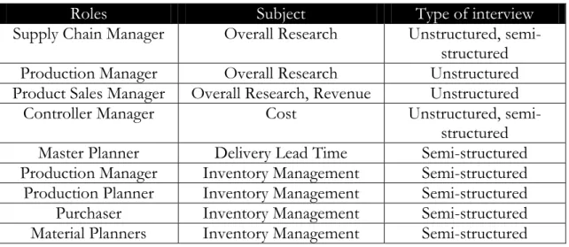
The different roles of the key informants, which subject area the questions regarded, and what type of interview that was used, are summarized in Table 2.2. No dates or times are included since interviews were held continuously throughout the whole research, often several times with the same employees.

Unstructured interviews

Theoretical understanding of the problem

Semi-structured interviews

(18)

Table 2.2. Interviewed key personnel.

Roles Subject Type of interview

Supply Chain Manager Overall Research Unstructured,

semi-structured

Production Manager Overall Research Unstructured

Product Sales Manager Overall Research, Revenue Unstructured

Controller Manager Cost Unstructured,

semi-structured

Master Planner Delivery Lead Time Semi-structured

Production Manager Inventory Management Semi-structured

Production Planner Inventory Management Semi-structured

Purchaser Inventory Management Semi-structured

Material Planners Inventory Management Semi-structured

2.4.3 Documents

Document sampling is one of six key methods for data collection (Yin, 1994). What types of documents that are included in the sampling can vary a lot. However, different types of document sampling are likely to be relevant in every case study (Yin, 1994). Before visiting the company, available information and documents that were to be found on the company‟s homepage were read in order to increase knowledge and credibility prior to the visit.

The document sampling that took place at the company was based on the first interviews with key personnel. The initial information that was given broaden the authors understanding of the problem and thus enabled further information to be gathered, such as financial data, inventory information, supplier agreements, and business process charts. The documents were primarily gathered from the company‟s ERP-system. However, this was combined intensely with interviews to cross-check the collected data, which is usually referred to as triangulation of both method and source (Williamson , 2002a). Indeed, it is important to validate that the gathered documents are in fact correct. As Yin (1994) states, the information gathered through document sampling should not be taken as the truth but be used to support other findings. Furthermore, increased validity and reliability was strived for by using more than one source to gather the same information.

(19)

2.4.4 Observations

Observations can be divided into two different types of observations; structured and participatory observations (Gillham, 2000). During a structured observation the observer takes an outside role and does not intervene with the objects being observed. The researcher thus watches from the „outside‟ in a carefully timed and specific way. The opposite of structured observing, which is participatory, involves the observer and is thus preferred in qualitative studies since the observer may ask questions and go more on depth.

Saunders et al. (2009) state that a participatory observation gives the observer the ability to perceive the reality from the viewpoint of someone „inside‟ the case study rather than external to it. Since the authors had the possibility to spend time and work closely with employees at the company, a lot of information were to be gathered in both formal and informal settings. Thus, making the authors more participant in their observations. The authors were however not conducting any labour themselves, but rather closely observed the work that was done. There were also observations made were the authors divided themselves in order to observe the issue from different perspectives, i.e. both from the „inside‟ and „outside‟.

There are some challenges related to participatory observations. When an observer is participant there is likelihood for biased information to be produced. The observer may become a supporter of the organization being studied and fails to set aside sufficient time to take notes and raise key questions (Yin, 1994). In order to avoid this biased behaviour the authors divided themselves so that one acted as an outside observer while the other participated. This enabled a more accurate observation since information was gathered both from „inside‟ and „outside‟ the observed group. However, this was not possible in every observation since both authors shared workspace with other employees.

(20)

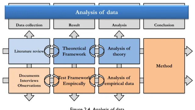
2.5 Analysis of data

In order to gain understanding and put focus on the right data, the authors analyzed the collected data continuously throughout the research process. This is something that is advocated by several authors according to Williamson & Bow (2002). When all data was collected the goal with the analysis was to incorporate the theoretical and empirical parts into a method. Looking at Figure 2.4 we can see how the data was collected and incorporated into a framework (See 3.5 Theoretical framework) that was tested empirically. These two parts were then analyzed together and concluded into a method. Both empirical findings and current theory forms the foundation of the DC-method.

Figure 2.4. Analysis of data.

As mentioned in 2.2 Research approach, the authors have used an abductive approach throughout the research. This have had an impact on how the research was carried out, including how the analysis was made. By analyzing the data continuously, there has been a possibility to go back and forth between the data collection and the analysis, which allowed the authors to focus on the right sources of information (both empirical and theoretical). For example, new aspects of the research could be identified when the empirical data was analyzed. These aspects were then investigated through literature reviews. One goal with the analysis was to find relationships between these different aspects and put them together in a framework which illustrates how different theories relate. The way of reaching conclusions have been discussed previously in 2.2 Research approach, and is referred to as systematic combining. By using both previously established theory and empirical findings the authors could build and test their framework. When analyzing qualitative data there are no strict rules to follow, however, some guidelines exist (Williamson & Bow, 2002). The overall goal with data analysis is to structure and bring meaning to the collected data, and thereby be able to

Conclusion Analysis

Data collection Result

Analysis of data Theoretical Framework Test Framework Empircally Documents Interviews Observations

Literature review Analysis of

theory

Analysis of empirical data

(21)

develop theory (Williamson & Bow, 2002). Through the case study and the literature reviews the findings were categorize into different subject areas and relationships could be identified. This is a common way of understanding the collected data and give the researchers deeper insights making it possible to find these relationships (Williamson & Bow, 2002). In the framework presented in 3.5 Theoretical framework, it is possible to see the relationships that were found when collected data was analyzed. The data analysis techniques that have been used are presented more thoroughly in the following subchapters.

2.5.1 Triangulation

Triangulation can be divided into different types of triangulation, whereof method triangulation and source triangulation are two of them (Williamson et al., 2002). The former analyzes the findings from different data collection techniques, e.g. do the answers provided in interviews correspond well with the data collected through document sampling? In terms of sources triangulation, it is about checking for consistency in the data retrieved from different sources, e.g. does the manager and subordinate provide the same answer when asked the same question? By applying both method and source triangulation in the research, the accuracy of the findings and conclusions are more likely to be high (Yin, 1994).

To exemplify: a lot of information was retrieved from Bosch Rexroth‟s ERP-system through document sampling. This information was then cross-checked with key personnel to ensure its credibility and accuracy. By doing this type of triangulation throughout the research, the authors could be more confident that the collected data was accurate. In fact, most of the qualitative data that are presented in this thesis was retrieved or cross-checked by the use of triangulation. Since the reliability and validity of the thesis depends greatly on how accurate the collected data is, it was seen as appropriate and necessary to apply triangulation in the research. Document sampling was the major data collection techniques in terms of retriving data, but was combined intensely with interviews to cross-check the reliability and validity of the collected data. This is usually referred to as triangulation of both method and source (Williamson , 2002a).

2.5.2 Pattern matching

As mentioned in 2.3.1 Analytical conceptual, analytical conceptual research has been used to develop the theoretical framework in this thesis. The theoretical framework has in parallel been evaluated against a case study. If the framework is

(22)

2.6 Validity and reliability

There are four different types of measures, or tests (Yin, 1994), that can be used to judge the quality of any given research design (Ellram, 1996). These four tests are external validity, reliability, construct validity, and internal validity (Yin, 1994; Ellram, 1996). However, in this subchapter the broader term “validity” will be used to describe external validity, construct validity, and internal validity, while the reliability will be investigated in its own. Saunders et al. (2009) state that validity is concerned with whether the findings are really about what they appear to be about, i.e. if the relationship between two variables is a causal relationship or if it is any other, unknown, variable that affects the result. The reliability, however, is used to investigate how well the result is consistent among different cases (Williamson, 2002a).

A high validity of the research is reached by the author‟s judgment and ability to present convincing arguments and facts, which later can be exposed to criticism from other scholars. However, by using proven and recommended approaches for the research design, consulting professors and professionals within supply chain to confirm correct interpretations, using multiple scholars to validate understandings and thoughts, the validity of the research is strengthened. More specifically, to assure a high validity in this research, triangulation of collected information, both through interviews and literature review, was of great importance. By interviewing multiple personnel about the same issue a wider understanding about the phenomena was given. Since all the persons that were interviewed had expertise in different areas of the organization, an even broader understanding was obtained. Moreover, since a qualitative research underlie the researchers own interpretation it is important to take measures to reduce the risk for biased results. In order to reduce this particular risk the authors divided themselves during interviews and observations to assure that the result was perceived equally from different perspectives. During observations, for example, one author could be a participating observer, i.e. more involved and asking questions, while the second author took notes and observed from a distance. The fact that the authors could conduct all the interviews in person further reduced the risk for potential misinterpretations. All the interview notes were also reviewed by the respondent after the interview to assure that the authors interpreted the information correctly. In order to assure a high reliability, a protocol can be developed containing the research instruments, rules followed during the research, and questions asked during the interviews (Yin, 1994). The methodological chapter in this research presents how the research was conducted and also specifies clear rules on how data was collected and analyzed. Thus, the method can be perceived as a protocol which strengthens the reliability.

Something that may affect the reliability negatively is the lack of information regarding which questions that were asked during the interviews. Since unstructured interviews were carried out there might also be a difference in how

(23)

different conclusions depending on which questions that are asked and how they are asked. To minimize this risk, the authors have specified that the initial interviews were unstructured, in order to get a theoretical understanding of the problem, and that upcoming interviews were more semi-structured. This was complemented with information regarding whom was interviewed, together with their professional title. The authors are convinced that these measures minimize the risk for different interpretations among scholars making the reliability and validity increase further.

(24)

3 Theoretical background

This chapter intends to give the reader a greater understanding of the theories related to the research problem in order to better understand the reasoning and arguments given throughout the thesis. Therefore, theories describing mapping of product structure and delivery lead time, placement of customer order decoupling point, and inventory management and cost will be of importance. Finally, the chapter relate the different theories to each other in a framework.

3.1 Development of theoretical framework

There are three primary parts of theory that will be described further in the theoretical background. These parts will then be combined into a theoretical framework that will form a key part during the rest of the thesis. The relationship between the research questions and theory is consolidated in Figure 3.1. The structure of the theoretical background follows the research questions in the sense that the topic of delivery lead time will be presented first, followed by relevant theory for CODPs, and its effect on inventory cost.

Develop a method for analyzing the relationship between delivery lead time and inventory costs

1. What determines a product’s delivery

lead time?

3.2 Mapping of delivery lead time

3.3 Feasible CODPs and factors affecting the choice of CODP

3.4 Inventory management and

cost

3.5 Theoretical framework 2. How are feasible

customer order decoupling points identified? 3. How are inventory costs affected by the position of the customer order decoupling point? R es earch q uestio ns T heor eti cal backg rou nd

(25)

The first two topics are closely related to different kinds of lead times and their effect on the CODP. There is however two more topic of relevance in the theoretical background, namely inventory management and costs. This part is primarily related to research question three. In order to answer this, knowledge regarding inventory management (e.g. for calculating potential safety stock) is important. To answer the first research question, theories regarding lead time, time-phased product structure, CODP, and factors for deciding CODP will be of interest. By going deeper and investigating these theories, which goes beyond determining a product‟s delivery lead time, there is more insight to be found that can be of value when answering the second and third research question.

To answer the second research question, knowledge of factors affecting the decision of CODP is of great relevance. By identifying the feasible CODPs it is possible to go on to research question three and answer how inventory costs are affected by the repositioning of the CODP. Depending on the chosen CODP the costs may vary. Therefore, explaining the relationship between the repositioning of the CODP and associated inventory costs is of high importance. How the theories relate to each other will be outlined in 3.5 Theoretical framework. The framework will incorporate all theory presented and form a key tool for the analysis that is presented in chapter 5.

3.2 Mapping of delivery lead time

The characteristics of a product desired by a customer and the offering by a company should be a match in order to create business (Lumsden, 2006). This of course include aspects of the product that are not related to its physical attributions, such as the time it takes to deliver the product. The offered delivery lead time may however be a mismatch with the customers demanded lead time, making even the best product unsellable. This scenario puts pressure to have a compelling delivery lead time in order to stay competitive and expand current market shares.

In order to establish a compelling delivery lead time a number of factors must be considered, such as the product‟s structure and the customer order decoupling point. The method for customer-driven purchasing (further called the CDP-method) by Bäckstrand (2012) focuses on these factors, among many others, in a thorough manner and outlines a total of 12 steps in 3 different phases. The first phase, constituting of five steps, have been of high relevance for this part of the

(26)

through the breadth and depth of its product structure (Olhager, 2003). A deep product structure indicates that a lot of operations and components are included in the final products. This often equates with a long production lead time, making it important to analyze different paths of the product structure to determine where inventory is appropriate to be kept and where highest reduction of lead time can be achieved (Olhager, 2003). Since focus is put on delivery lead time, the depth of the structure is of greater relevance than the breath of it.

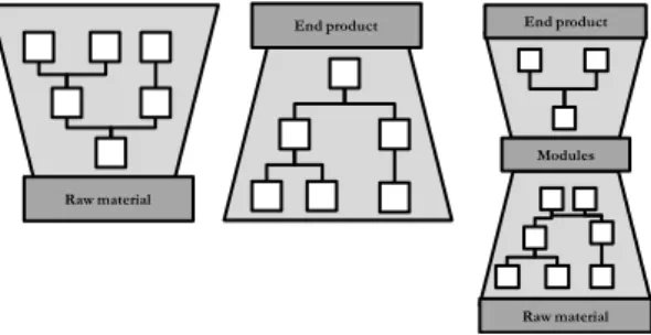
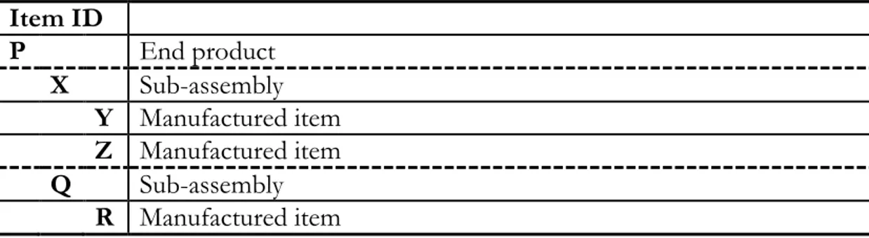
The included components and materials in a product structure are to be found in a bill-of-materials (Clark, 1979; Hegge & Wortmann, 1991), also known as a BOM. When illustrating a product structure, the end product (See P in Figure 3.2) is displayed at the top of a hierarchy with included components and raw materials following. Each component that is completed in subassembly has one or a few including items in its hierarchy that together form the structure of that particular component, as seen under component X in Figure 3.2.

Figure 3.2. Product structure of the end product P. Illustration based on Bäckstrand (2012, p. 63)

The term „material profile‟ is as well used when describing the products structure (Olhager, 2003; Wikner 2014). When the product structure, or material profile, is converging, as seen in Figure 3.2, several subassemblies and components are combined into an end product. There are however other structures that may be used as well. A diverging structure is opposite of the converging structure, meaning that a raw material is transformed into several different products (Bäckstrand, 2012). In modularized production a combination of both converging and diverging structure is to be found. Modules are produced from several components and materials, these modules can later be assembled and form various products. Other scholars, e.g. Olhager & Wikner (1998), refer to these material profiles as VAX-profiles, where V describes the divergent, A the convergent, and X the combination of these (See Figure 3.3).

Figure 3.3. VAX material profiles. Illustration based on Bäckstrand (2012, p. 63). P X Y Z Q R End product Raw material Modules End product Raw material

(27)

For an easier visualization of the product structure, an indented BOM is used. The including components are displayed just as in a regular BOM (which is more detailed) and as in the material profiles seen in Figure 3.3, but with a clearer overview. The indented BOM illustrated in Table 3.1 displays how the included components are related to the end product P. Even though Table 3.1 does not display any information regarding lead times there is a possibility to include this in future stages, when the information is known and processed (See e.g. p. 192 in Wikner (2014)).

Table 3.1. Indented BOM on product structure in Figure 3.2.

Item ID P End product X Sub-assembly Y Manufactured item Z Manufactured item Q Sub-assembly R Manufactured item

There is, however, not enough information in the displayed indented BOM or a hierarchical product structure to motivate a decision regarding reduction of delivery lead time. By transforming the product structure and a detailed BOM to a time-phased product structure, a visual representation of a product‟s aggregated lead time can be developed (Clark, 1979). The time-phased product structure can then be used to further investigate how the delivery lead time may be reduced. This is related to the second step of Bäckstrand‟s (2012) CDP-method, which is to define the supply lead time for each included component and material.

3.2.2 Different types of lead time

In a production flow, different terminologies of lead time are used to specify which part of the flow one particular lead time refers to. Before going further into the time-phased product structure, where this terminology is used, these terms will be explained.

Delivery lead time

The delivery lead time (D) is defined as the time from the receipt of a customer order to the delivery of the product (APICS, 2005, p. 29). One synonym to

(28)

Important to note is that when referring to delivery lead time in chapter 4 Empirical data and chapter 5 Analysis, it is defined as the time from the receipt of a customer order to the delivery of a product into the finished goods inventory. Thus, the last part of the delivery lead time, from the finished goods inventory to the customer, is not included.

Demand lead time

The delivery lead is described as the time between a customer order is received and delivered. The demand lead time, on the other hand, is the amount of time potential customers are willing to wait for the delivery of a good or a product (APICS, 2005, p. 30). One synonym to this term is customer tolerance time.

Supply lead time

The supply lead time is the total time it takes to restock a product (Bäckstrand, 2012). In the supply lead time the focal company‟s internal lead time and external lead time is included. When identifying the length of the total supply lead time the lead time of each item is of great importance. The BOM (with included information of lead time) is basically illustrated horizontally in order to display the time on the x-axis. By allowing the lead time for each item to form a horizontal arrow, or line, the total supply lead time can be mapped out, as seen in Figure 3.4.

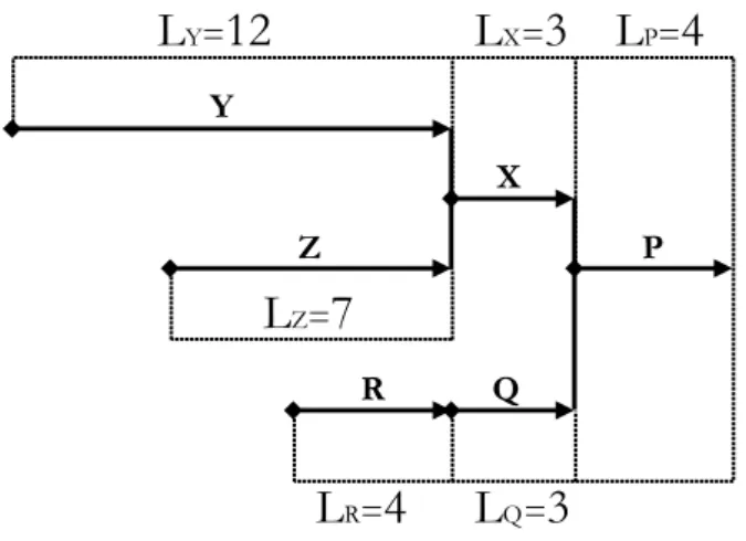
Figure 3.4. Time-phased product structure for the end product P. Based on Bäckstrand (2012, p. 99).

The lead time for each component is marked with L in Figure 3.4. The supply lead time is however not displayed in full. Nevertheless, by calculating the longest leg in the time-phased product structure the total supply lead time can be calculated (Bäckstrand, 2012). In Figure 3.4 the longest leg is through P, X and Y, making the total supply lead time of 19 (4 + 3 + 12). The technique of time-phasing is similar to traditional Gantt charts and has a long history of customizations to it.

P X Y Z Q R

L

P=

4 L

X=

3 L

Y=

12 L

Z=

7 L

Q=

3 L

R=

4

(29)

3.2.3 Customer order decoupling point and the S:D ratio

The CODP is the point where the forecast-driven activities are separated from the order-driven (Giesberts & van de Tang, 1992). In MTS companies the delivery lead time is short, thus having the CODP closer to the end customer. In ETO companies the delivery lead time is much longer and consequently having the CODP much higher upstream from the end customer.

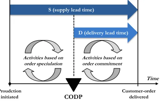
All the definitions regarding the CODP are in one way or another based on the ratio of production lead time (P) and the delivery lead time (D). The concept of the P:D ratio was first introduced by Shingo (1981). It was however presented to a broader audience by Mather (1984). In 1984 the relationship was between production (P) and delivery lead time (D), thus the P:D ratio. This will however be referred to as S:D ratio further on since the relationship investigated in this research is between supply lead time (S) and delivery lead time (D). The use of S and D instead of P and D is inspired by Wikner & Rudberg (2005). The concept of S:D ratio is exemplified in Figure 3.5.

Figure 3.5. Concept of the S:D ratio illustrated with the CODP. Based on Wikner & Rudberg (2005, p. 213).

As seen in Figure 3.5, the activities pre the CODP is based on speculation while

S (supply lead time)

D (delivery lead time)

CODP

Time

Proudction

initiated Customer-orderdelivered

Activities based on order commitment Activities based on

(30)

other factors. There is, however, a possibility to adjust the positioning of the CODP in order to achieve a shorter delivery lead time (D).

3.3 Feasible CODPs and factors affecting the

position of CODP

Where to strategically move the CODP can be answered by incorporating the theories of CODP with the time-phased product structure, since it clearly illustrates where, as Wikner & Rudberg (2005) calls them, feasible CODPs may be positioned. Moreover, Olhager (2003) presents a couple of factors that affect the positioning of CODP, or the positioning of the order penetration point (OPP), as called in Olhager (2003). These are divided into three types of categories, namely market-related factors, product-related factors, and production-related factors, all of which need to be considered before choosing between the feasible CODPs. Each factor within these three categories are presented further, in order to ensure greater understanding of them.

3.3.1 Market-related factors

The market sets the ultimate goal for how the production should be structured. If the market‟s needs for the product are not met, the product will be unsuccessful. The first factor affecting the positioning of the CODP is the requirement of delivery lead time. It is the market that restricts how far backwards the CODP can be positioned. The further back the CODP is positioned, the longer is the delivery lead time, and vice versa. Next factor for positioning the CODP is product demand volatility. Low volatility means that the production can be forecast driven while a high volatility makes forecast difficult and pushes the production to produce on actual customer order. Closely related to demand volatility is product volume. Depending on where in a product‟s life cycle the product is, different characteristics become more important than others. Early in the product‟s life cycle, the delivery, design, and flexibility can be more important, while price may be of higher importance in the end of the product‟s life cycle. A broad product range and product customization, which is the next factor, pushes the production toward MTO since it is very costly to fulfill orders on a MTS basis. The factors of customer order size and customer order frequency are also of importance since frequent orders are easier to forecast and thus makes an order-fulfillment strategy based on MTS possible. When the orders are more frequent it is also possible to decrease the order sizes, which further facilitates the forecasting. High seasonal demand may motivate that companies manufacture some components to stock in periods of lower demand, in order to assemble it on an ATO basis (Olhager, 2003).

3.3.2 Product-related factors

How the product is designed plays an important role in how to position the CODP. If few components are needed in order to finalize the product, a MTS

(31)

strategy may be appropriate, meaning that the CODP is downstream, closer to the end customer. The first product-related factor mentioned in Olhager (2003) is modular product design, which often is developed from the customer‟s requirement of short delivery lead time and high variety in product. In cases with high modularity order-fulfillment according to ATO is common. The customization opportunities given to the customer is also a factor to consider. With customization opportunities close to the end customer, production on an ATO basis is appropriate. This is however not possible when the customization occurs in early stages of the production. A production according to MTO is then appropriate. The last product-related factor is the product structure. A broad and deep product structure is more complex and corresponds to a long cumulative supply lead time since more activities are needed in order to finalize the product. The task of analyzing feasible positioning of the CODP becomes more challenging in these cases, since a more complex product structure needs to be analyzed (Olhager, 2003).

3.3.3 Production-related factors

The single most important factor to consider within the production-related factors is the production lead time. Long production lead times push production towards MTS since customers generally are not willing to wait for the product to be made. By reducing the production lead time itself there is a possibility to either reduce the delivery lead time and thus offer a better deal, or keep the delivery lead time and reduce the number of activities that are forecast-driven. The number of planning points is another factor to consider. (Olhager, 2003). Since the CODP cannot be positioned in an activity, it is only possible to position it in either a buffer before or after the activity (Wikner & Rudberg, 2005). The number of planning points constrain where the potential CODP can be positioned. An automated and dedicated line can be seen as a single process and thus enabling only two feasible positions of the CODP, either before or after the process. A job shop, on the other hand, gives the possibility to choose position for the CODP to a much higher extent. The flexibility of production processes and the bottleneck are two factors that require consideration. The bottleneck for example is preferred to be positioned upstream the CODP since it is protected from volatility in demand, in contrast to being positioned downstream the CODP. Resources that are sequence-dependent should also be positioned upstream the CODP since the flexibility of resource is lower and can thus turn into bottlenecks without proper sequencing (Olhager, 2003).

(32)

Figure 3.6. Feasible time-phased positions of the CODP. Based on Wikner & Rudberg (2005).

The CODP continuum contains all the possible positions for the CODP between the two extreme points, MTO and MTS. This is illustrated by a rounded square with thin black lines and is to be found in the top of Figure 3.6. Where there is a natural phased decoupling point to be found throughout the whole time-phased product structure (point 1, 2, 3, and 6) a feasible CODP is identified. A quasi-feasible CODP is instead identified when one part of the flow has a natural time-phased decoupling point while other part of the flow does not, as illustrated by point 4 and 5. In these cases there is not recommended to position the CODP since it does require more speculation with limited positive effects on the total delivery lead time. The positions of 1, 2, 3, and 6 do however have natural time-phased decoupling points throughout the whole structure, making it possible to position the CODP in these points and thus decouple the forecast driven production from the customer-order driven production.

3.4 Inventory management and costs

As mentioned earlier the CODP is the point where the forecast-driven production is separated from the order-driven. One reason for this is to handle disturbances easier, usually done by building a stocking point at the CODP (Wikner, 2014). This subchapter will describe how inventory can be managed and which costs that may be connected to keeping inventory.

3.4.1 Costs associated with inventory

If an analysis is to be made between delivery lead time and inventory cost it is necessary to calculate accurate cost of keeping inventory. There are two fundamental costs related to keeping inventory, carrying costs and ordering costs (Olhager, 2013). P X Y Z Q R MTO ATO MTS 6 5 4 3 2 1 Production initiated CODP Customer order finished D S CODP continuum Feasible CODP’s Quasi-feasible CODP’s Time-phased process

(33)

Inventory carrying costs

The primarily cost related to inventory carrying costs is the cost of tied up assets (Mattsson, 2010). Furthermore, costs associated with material handling, inventory rent, insurance, and obsolescence are included. The later costs are dependent on if the inventory is rented or owned by the company. If the inventory is rented, these costs are usually variable and depend on how much that need to be stored (Axsäter, 2006). If the inventory is owned by the company, these costs can be seen as fixed given that an increased volume fits into the current inventory (Mattsson, 2010). Furthermore, costs of obsolescence are somewhat affected by the inventory

levels. The inventory carrying costs (Cc) are calculated by the formula (Olhager,

2013):

Cc = r * V

The carrying charge (r) can be based on the money rate if the money invested in inventory has been borrowed from a bank (Axsäter, 1991). It can also be based on the minimum acceptable rate of return a company demand (La Londe & Lambert, 1977). In such cases, the investments in inventories should result in a rate of return equal to other possible investments. The value of item (V) is the value an item has according to the inventory accounting (Mattsson, 2010) and can be based on either actual costs or standard costs depending on which accounting system being used (Magee & Boodman, 1967).

Ordering costs

These costs are dedicated to each specific order and arise every time a new order is put (Axsäter, 1991). The primary cost is the administrative ordering cost, i.e. the cost for releasing an order and handling documents associated with an order release (Olhager, 2013). Other costs included in the ordering costs are production costs for setups, transportations, handling, and such (Axsäter, 1991).

3.4.2 Fixed-order quantity models

There are different methods used to manage the inventory depending on the prerequisites a company has. In general a distinction is made between fixed-order quantity models (Q-models) were the order quantity is the same but with different intervals between the orders, and fixed time-period models (P-models) were the orders are placed within the same intervals but with different quantity (Jacobs,

(34)

In Q-models there are two things to consider; how much to order every time (order quantity) and when to order, i.e. at which inventory level it is necessary to order (Oskarsson et al., 2006). The order quantities can be calculated using the economic order quantity formula (EOQ-formula) also called the Wilson-formula. The purpose with the Wilson-formula is to find the order quantity that brings the lowest costs, hence the name economic order quantity (Oskarsson et al., 2006). With an increased quantity, the carrying costs increase and the ordering costs decrease. Looking at the opposite, lowering the order quantity results in lower carrying costs, but higher ordering costs. The goal with the Wilson-formula is to find the optimal order quantity with respect to these costs.

Some assumptions need to be considered when the Wilson-formula is applied. First of all, an even consumption is a prerequisite for the calculations to be valid (Oskarsson et al., 2006). Thus, the mean inventory is calculated as the order quantity divided by two. Furthermore, no quantity discount is included, no capacity limitations are considered, and everything is assumed to be delivered at the same time, i.e. the whole quantity is delivered at the same time (Oskarsson et al., 2006). Before the Wilson-formula is presented, the calculations behind inventory carrying costs and ordering costs will be presented. The yearly inventory

carrying costs (Cc) are calculated as (Oskarsson et al., 2006):

Cc =

r = carrying charge

V = value of item in specific inventory Q = order quantity

The yearly ordering costs (Co) are calculated as (Oskarsson et al., 2006):

Co =

O = ordering cost D = annually demand Q = order quantity

D/Q = number of orders a year

The total cost of inventory is thus calculated as (Oskarsson et al., 2006):

(35)

To calculate the EOQ, the following formula is used (Oskarsson et al., 2006): EOQ = √( ) ( )

Safety Stock

The size of the inventory is based on a known demand, but in reality the real demand rarely correspond exactly to the anticipated demand (Oskarsson et al., 2006). Due to this, there is a need for companies to have safety stocks. Safety stocks are used to protect from stock outs if the consumption becomes larger than expected or the supplier lead time becomes longer than anticipated. Fluctuations in supplier lead can, however, also be managed with safety lead times. The size of the safety stock can be calculated by something called SERV1, which is based on the probability to avoid stock outs between two orders (Oskarsson et al, 2006). To use SERV1, the demand and supplier lead time are presumed to be normally distributed. To guard against unexpected increase in demand during the supplier lead time, the following formula is used:

SL = k x σ x √LT k = safety factor

σ = standard deviation in demand during the supplier lead time LT = expected supplier lead time

Standard deviation (σ) is a statistical measure that shows how the real demand deviates from the expected (forecasted) demand (Oskarsson et al., 2006). The safety factor (k) is decided by the company and is based on the desired service level (i.e. the probability to be able to deliver directly from inventory). The service level can in turn be selected based on an ABC-classification. The ABC inventory classification makes a distinction between the importance of stored items allowing the control of each items to be adapted based on its importance (Arnold et al., 2008). By doing this differentiation, different service levels can be selected based on the importance of each item. When the desired service level is selected, the safety factor is retrieved from the following table:

Table 3.2. Service level and Safety factor.

Feasible customer order decoupling points and associated inventory costs