Matching Feature Points in 3D World

Postadress: Besöksadress: Telefon:

Matching Feature Points in 3D World

Blerta Avdiu

THESIS WORK 2012

Electrical Engineering with Specialization in

Embedded Systems

Postadress: Besöksadress: Telefon:

Matching Feature Points in 3D World

Blerta Avdiu

This thesis work is performed at Jönköping University, School of Engineering, within the subject area Electrical Engineering. The work is part of the two year master’s degree program with the specialization in Embedded Systems.

The author is responsible for the given opinions, conclusions and results.

Examiner: Professor Shashi Kumar University Supervisor: Alf Johansson Company Supervisor: Göran Calås Scope: 30 credits (D-level)

Abstract

This thesis work deals with the most actual topic in Computer Vision field which is scene understanding and this using matching of 3D feature point images. The objective is to make use of Saab’s latest breakthrough in extraction of 3D feature points, to identify the best alignment of at least two 3D feature point images. The thesis gives a theoretical overview of the latest algorithms used for feature detection, description and matching. The work continues with a brief description of the simultaneous localization and mapping (SLAM) technique, ending with a case study on evaluation of the newly developed software solution for SLAM, called slam6d.

Slam6d is a tool that registers point clouds into a common coordinate system. It does an automatic high-accurate registration of the laser scans. In the case study the use of slam6d is extended in registering 3D feature point images extracted from a stereo camera and the results of registration are analyzed.

In the case study we start with registration of one single 3D feature point image captured from stationary image sensor continuing with registration of multiple images following a trail.

Finally the conclusion from the case study results is that slam6d can register non-laser scan extracted feature point images with high-accuracy in case of single image but it introduces some overlapping results in the case of multiple images following a trail.

Keywords

Simultaneous Localization and Mapping (SLAM) 3D Scene

Iterative Closest Points Algorithm (ICP) Global Matching

Content

1 INTRODUCTION... 1

1.2 BACKGROUND ... 1

1.3 PURPOSE AND RESEARCH QUESTIONS ... 3

1.4 DELIMITATIONS ... 3 1.5 OUTLINE ... 4 2 THEORETICAL BACKGROUND ... 5 2.1 COMPUTER VISION ... 5 2.1.1 Image Acquisition ... 5 2.1.2 Pre-processing ... 6 2.1.3 Feature Extraction ... 7

2.1.4 Detection and Segmentation ... 9

2.1.5 High Level Processing ... 10

2.1.6 Decision Making ... 10

2.2 FEATURE EXTRACTION ALGORITHMS ... 10

2.2.1 Edge Detection Algorithms ... 10

2.2.2 Corner Detection Algorithms ... 12

2.2.3 Speeded-Up Robust Features (SURF) ... 16

2.3 REAL-TIME IMAGE PROCESSING ... 19

3 SIMULTANEOUS LOCALIZATION AND MAPPING (SLAM) PROBLEM ... 20

3.1 SLAM FROM A HISTORICAL PERSPECTIVE ... 20

3.1.1 Essential Formulation and Structure of the SLAM Problem ... 21

3.1.2 Solutions to the SLAM Problem ... 22

3.2. 3DTOOLKIT ... 23

3.2 ALGORITHMS WITHIN SLAM6D... 23

3.2.1 Iterative Closest Point Algorithm – ICP ... 23

3.2.2 Global Matching ... 26

3.3 THE SHOWCOMPONENT OF 3DTK ... 28

4 RESEARCH METHODS ... 29

4.1 CASE STUDY RESEARCH ... 29

4.1.1 Data Collection Methods ... 29

4.2 TEST PLAN ... 30

5 CASE STUDY AND RESULTS ... 32

5.1 OVERVIEW OF PROCESSING ... 32

5.2 DATA PREPARATION ... 33

5.3 RESULTS OF MATCHING ... 35

5.3.1 Matching Single Image, Stationary Image Sensor ... 35

5.3.2 Matching Multiple Images, Moving Image Sensor ... 36

5.3.3 Global Matching of Multiple Images ... 38

5.3.4 Interpretation of the Results ... 40

6 CONCLUSIONS AND FUTURE WORK ... 42

6.1 CONCLUSIONS ... 42

6.2 FUTURE WORK ... 42

1

Introduction

This project has been carried out at the Swedish Company called Saab Training Systems (STS).

Saab AB is the main Swedish company that serves the global market with the world-leading technology solutions, services and products from military to civil security. This company operates on every continent and has in total six business areas:

 Aeronautics

 Dynamics

 Electronic Defense Systems

 Security and Defense Solutions

 Support and Services

 Combitech

All these areas are divided in divisions and the STS is one of the main division in the business area Security and Defense Solutions.

Saab Training Systems (STS) is the part of the company which is the leading supplier of training systems for the army, the air force and the navy. (STS) develops,

manufactures and markets military training systems including tactical training, mobile data communication systems, different types of laser simulator systems and facilities for the training of combat in urban environments.

1.2 Background

Generally if we take into account the complexity and the dynamics of life in the world during the last decade’s national security and civil security has become a key factor for many developed countries. More and more countries have thrown over the idea of having heavy personal defense system to professional military defense system that is built around small, well trained forces with greater mobility, enabling the response and counter of a threat before it reaches its own territory.

The development of the technology nowadays is leading towards the use of robots instead of humans in many areas of industry in which the level of risk is very high. Interest for robotic systems is increasing in many other fields too, from academic to commercial areas, from security and defense to entertainment applications. Robotic systems must deal with several fundamental issues, such as motion estimation, 3D scene reconstruction, object tracking, navigation and so one. Making the robot see and understand the environment by using smart cameras is a high level issue in computer vision field.

Three dimensional (3D) scene understanding is one of the main goals in computer vision and robotics. Thus, here exists a wide body of work and applications in both areas.

Saab has spent the last seven decades developing technology with the purpose of preparing and protecting both society and its individuals. It is one of the main

companies in the world that serves the global market of governments, authorities and corporations with products, services and solutions ranging from military defence to

civil security. Being prepared for the non-static scenarios, knowing in advance, training the soldiers while making the training environment as real as possible with the war scenarios by using different types of simulation systems like audio and video images, image based navigation systems, etc.

One of the projects inside Innovation Labs, the department inside STS is called Image Based Navigation (IBN). Generally, the main goal of the project was to achieve a complete navigation system that can handle all cases of 3D, capable to fill gyro requirements without gyro and provide a 3D model of the environment. The requirements behind the IBN system were:

 From two images estimate the relation between these two camera positions, rotation and translation.

 Define an algorithm for real time navigation based on images taken from camera.

 Define the 3D information that is available and the quality of the measured data.

To fill these requirements the first problem was how to find objects or points of interest that are represented within images. Here exist a wide range of algorithms that can be used for detecting features in the images depending on the nature of the problem. These algorithms that give 2D feature information in the images are the algorithms for corner and line detection, algorithms based on convolution and Fourier Transforms, matching based in the image properties like frequency, color, shape etc. The algorithm developed within STS can detect the image features called feature points and can give a description (identification) for each feature point all this using stereo images. After that, the system can match these features to a global coordinate system and also can estimate the camera position based on the information from current position and next position with a grade of uncertainty. As camera moves in an unknown environment taking the observations of the environment by producing feature points which are correlated with each other because of the common error in estimating the camera position. This error becomes bigger and bigger and after the camera has moved in a longer path or after it comes back to the same position (start position) due to continuously increasing error it will give wrong results. This is called the loop closure problem. Different algorithms use different methods to solve this problem but there isn’t any concrete solution for this issue.

Image processing has been considered as an imprecise science but new algorithms for image analysis and the mathematical solutions for the properties between images have had a rapid evolution in recent years.

With this project we will evaluate one of the latest developed solutions for SLAM (Simultaneous Localization and Mapping) problem called slam6d when using the achievements of the STS’s latest breakthrough in feature point detection.

SLAM is a problem which tries to solve the possibility of building a consistent map of the environment and at the same time use this map to compute its location by placing a mobile robot in an unknown environment and location. After theoretical and

conceptual formulation of the SLAM problem there has been developed a number of algorithms and implementation solutions. Slam6d is one of the software based solutions to SLAM which will be used in the case study.

1.3

Purpose and Research Questions

The thesis targets evaluation of software based solutions for 3D environment reconstruction based on consecutive images consisting of input data in the form of 3D oriented feature points, e.g. 300 points per image. The objective is not to identify feature points as this step is already provided as input data for further analysis.

The objective of the thesis is to make use of Saab’s latest breakthrough in image 3D feature point analysis to create a function which is able to:

 Identify the best alignment of at least two separate 3D point images (A, B) each consisting of approximately 300 feature points described as (x, y, z coordinates, or equivalent format), thus constructing a new 3D image C.

C should have the properties that A  BT is given the best possible alignment match while extending the scene C to be defined as A  BT where BT is coordinate translated B.

 Processing of multiple images is repeated using Cn as the new A, and B as the new image to be integrated in the new scene Cn+1

 During the 3D scene image discovery process, the best real-time method

(algorithm) to be proposed is to take into consideration that images will contain biased data which needs to be discriminated.

The thesis will include the following steps:

1. Survey and analysis of existing methods for 3D SLAM, and real-time 3D reconstruction based on 3D (feature) points.

2. Defining and implementing method evaluation tool framework.

3. Implementing and evaluating methods, algorithms for real-time synthesis of 3D environment based on consecutive 3D images based on the following scenarios:

a. Stationary 3D image sensor.

b. Moving 3D image sensor (known movement).

c. Consecutive movement of 3D image sensor following a trail. d. Consecutive movement of 3D image sensor following a loop, thus

needing to integrate with old image points.

e. Generation of mixture of image intensity data with generated 3D scene model.

f. Optional: Stationary 3D image sensor with a moving object interfering with the scene.

4. Evaluation and suggestion of most suitable real-time solution for 3D scene generation, executable on a standard PC.

1.4

Delimitations

This thesis work will not include own developed algorithm that will lead to a new software platform for simultaneous localization and matching of the feature point images. This is a limitation due to the complex nature of the problem and the time limitations.

The other limitation is that while running tests for getting the input data the moving objects and the reflected objects that in real time interfere with the scene are removed to simplify the work and analysis.

1.5

Outline

The rest of the report is organized as follows: Chapter 2 provides a general theoretical background in the features and the mostly used feature extraction algorithms; Chapter 3 gives a brief overview of the SLAM problem and the 3D Toolkit method that solve this problem; Chapter 4 contains the chosen research method and motivations of this choice; Chapter 5 describes the case study results and interpretation of the results when using slam6d; finally conclusion and future work is given in Chapter 6.

2

Theoretical Background

This chapter gives a brief introduction to the mostly used methods, algorithms for detecting, describing and matching images in computer vision.

It starts with a short description of the computer vision tasks in image processing while detecting interest points, gives a clear definition of the image feature points to continue with a brief explanation of the algorithms used for detecting these features. Chapter 3 will give some more detailed information for the theories behind the SLAM (Simultaneous Localization and Mapping) problem formulation that we have taken into consideration during the analysis in the case study.

2.1

Computer Vision

Computer vision is the science and technology of the machines that see, the machine can do automated processing of images from the real world to extract and interpret information on real time basis. In short, computer vision deals with the theory behind artificial systems that extracts information from images.

There exist a wide range of domains and sub-domains where computer vision seeks to apply its theories and models to construct computer vision systems.

Typical tasks of computer vision are:

 RECOGNITION in image data: object recognition, content-based image retrieval, pose estimation, optical character recognition, and facial recognition.

 MOTION analysis:

Egomotion: determines the 3D motion of the camera within an environment. Tracking: how to follow the moving objects in the image.

Optical flow: for each point in the image determines how that point is moving

relative to the image plan.

 SCENE RECONSTRUCTION by computing a 3D model of the scene from one or more images of the scene.

 IMAGE RESTORATION: As the name states for, has to do with the removal of noise and other supplements from images.

 3D VOLUME RECOGNITION: reconstruction of the 3D volume from 2D images.

Performing these tasks requires different methods, algorithms and unique functions characteristic for computer vision systems to be used. Some of the typical functions of the computer vision systems are: image acquisition, pre-processing, feature extraction, detection/segmentation, high-level processing, decision making.

2.1.1 Image Acquisition

Image acquisition is the digitization and storage of an image. The images we process in computer vision are formed by light bouncing off surfaces in the world and into the lens of the system.

A digital image is produced when this light hits an array of image sensors inside the light-sensitive cameras. Each sensor produces electric charges that are read by an

electronic circuit and converted to voltages. These are in turn sampled by a device called a digitizer (analogue -to-digital converter) to produce the numbers that the computer processes, called pixel values. Thus, the pixel values are rather indirect encoding of the physical properties of visible surfaces. The pixel values typically correspond to light intensity in one or several spectral bands (grey images or color images), but it can also be related to various physical measurements, [1], [2], [3]. There exist three main principal sensor arrangements used to transform illumination energy into digital images:

 Single imaging sensor

 Line sensor

 Array sensor.

Image Acquisition Using Sensor Arrays: This is the predominant arrangement of

the sensors found in digital cameras, other light sensing instruments, numerous electromagnetic and some ultrasonic sensing devices. Here individual sensors are arranged in the form of a 2-D array; a typical sensor for this acquisition method is a CCD (charged coupled device) array, which can be manufactured with a broad range of sensing properties and can be packaged in rugged arrays of 4000 x 4000 elements or more [1] The principal manner in which array sensors are used is shown in the figure 2-1.

Figure 2-1. Digital image acquisition using sensor arrays.

2.1.2 Pre-processing

Image pre-processing uses some operations which sup-press information that are no relevant to the specific image processing methods and enhance other image features important for further processing with a specific computer vision method that is going to be applied to image data, as the following examples:

 Re-sampling in order to assure that the image coordinate system is correct.

 Noise reduction in order to assure that sensor noise does not introduce false information.

 Contrast enhancement to assure that relevant information can be detected.

 Scale-space representation to enhance image structures at local appropriate scales [3].

2.1.3 Feature Extraction

Feature extraction is one of the function’s that is interesting for our work in the rest of the report. We use special feature points to extract the redundant information from the images and process them further to construct a 3D scene of the environment.

The concept of features is very general and there is no universal definition, therefore the choice of features particularly in computer visions is highly dependent on the nature of the problem. They are used as start point of many computer vision

algorithms. We can think of features as specific parts of image ranging from simple structures such as edges, corners, interest points, and regions of interest points to more complex structures such as objects (ridges).

Edges: are points where there is a boundary (or an edge) between two image regions.

In general, an edge can be of almost arbitrary shape, and may include junctions. In practice, edges are usually defined as sets of points in the image which have a strong gradient magnitude.

Edge pixels are pixels at which the intensity of an image function changes sharply,

and edges (edge segments) are sets of connected edge pixels. Edge detectors are image processing methods designed to detect edge pixels. Edge detection is the approach used most frequently for segmenting images based on sharply local changes in intensity [1].

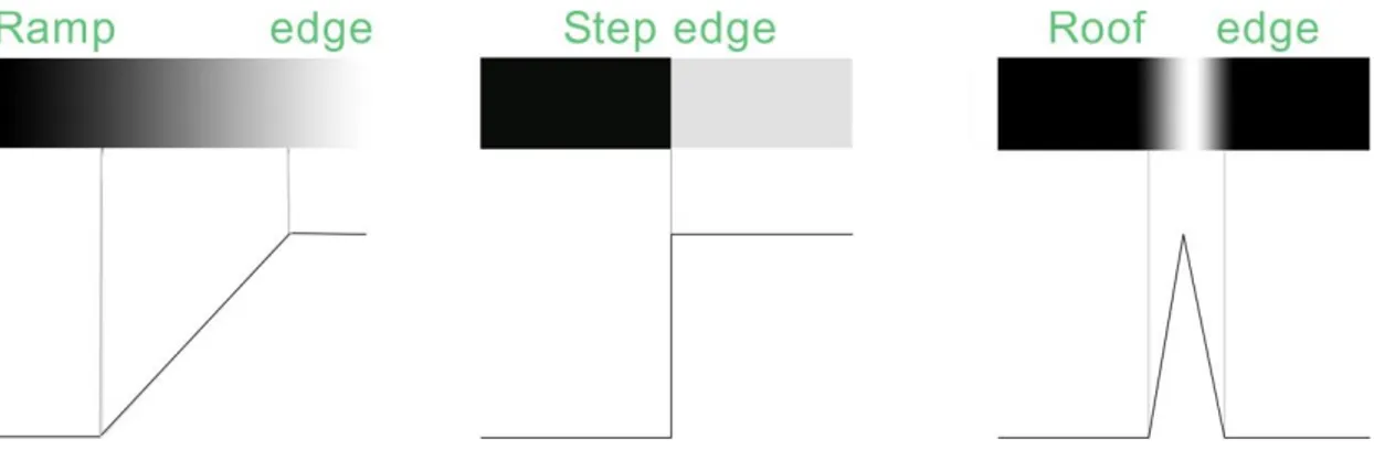
Edge models are classified according to their intensity profiles:

A step edge: This includes a transition between two intensity levels occurring ideally

over the distance of 1 pixel. This clean, ideal edges occurs over the distance of 1 pixel, with no need of additional processing (such smoothing) to be used to make them look “real”. Step edges occur in images generated by computers for use in areas such as animations see figure 2-2 (b) [1].

A ramp edge: In practice, digital images have edges that are blurred and noisy. In

such situations edges are modelled as having an intensity ramp profile, see figure 2-2 (a). This model has no longer a thin (1 pixel thick) path. Instead, an edge point now is any point contained in the ramp [1].

A roof edge: This is the third model of an edge as illustrated in figure 2-2 (c). Roof

edges are models of lines through a region, with the width of a roof edge determined by the thickness and sharpness of the line [1].

Corners and Interest Points: The terms “corners”, “edges”, “interest points”,

“features” are used interchangeably in literature, thus confusing the issue.

After the definition of the edges the term corners – the point where two nonparallel edges cross each other comes into consideration. A corner can also be defined as two dimensional points for which there are two dominant and different edge directions in the local neighborhood of the point. Practically the name “corner” is features formed at boundaries between only two image brightness regions, where the boundary curvature is sufficiently high [4].

Interest points: They are points (pixels) in images which have special properties that

distinguish them from its neighbouring points and they are likely to be found in other images of the same object from different view. An interest point can be a traditional corner like L, Y, X, T, but it can also be a point in a locally maximal curvature, an isolated point of local intensity maximum or minimum, a line end. Approaches for interest points detection are widely used in image processing, most of the methods created to detect corners, generally they detect interest points rather than corners but the term corners is used traditionally. Due to their distinctive nature interest points plays an important role in object recognition, matching of two different stereo views, tracking and motion estimation. Brief information about interest point extraction will be added in section 2.2.

Figure 2-3. Interest points, to the left original image to the right image with corners.

Blobs (Regions of interest or interest points): The aim of blob detection in

computer vision area is to detect points and/or regions in the image that differ in properties like brightness or color compared to the surrounding, see figure 2-4.

The main reason for studying and developing blob detectors is that blobs provide complementary description of image structures in terms of regions, which is not obtained by edge detectors or corner detectors. Blob detection is used to obtain regions of interest for further processing. These regions are than interesting information for the field like object recognition/tracking, segmentation, as main primitives for texture analysis and texture recognition, very popular use as interest points for wide baseline stereo matching recently. Blob detection methods are:

 Determinant of Hessian (DoH)

 Difference of Gaussian (DoG)

 Laplacian of Gaussian (LoG)

 Maximal stable extremal regions (MSER).

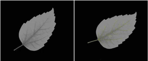
Ridges: The notion of ridges extends the concept of local maximum of a given

function, see figure 2-5. For a function of two variables ridges are a set of curves whose points are a local maxima of the function in at least one dimension. For a function of N variables the ridges are a set of curves whose points are the local maxima of the function in N-1 dimensions.

The concept of ridges appears really often in image analysis, especially in the fields for road extraction in aerial images and for extracting blood vessels in medical

images. Even if it is algorithmically hard to extract ridge features from general classes of gray-level images than edge, corner, blob features in the area of medical image processing is done a lot of work for ridges, ridge core theories and their applications.

Figure 2-5. Ridges, to the left original image and to the right image with ridge.

2.1.4 Detection and Segmentation

When we do image processing we can decide if the output after the processing will be an image again or an attribute extracted from the input image. Segmentation and detection are two major steps in this direction.

Segmentation is the case when we divide the image into some objects or regions that we are interested to analyze further. In image segmentation thresholding is the most commonly used method due to its simplicity and computational speed. The output of a thresholding process is a binary image, where black pixels describes the background and white pixels describes the foreground (objects) or vice versa.

Detection is the process when different algorithms are used to detect lines, edges, corners, feature points, point clouds. For more details about the detection algorithms see the section 2.2 of this chapter.

2.1.5 High Level Processing

This is the step that comes after low-level processing like feature extraction, detection and image segmentation. At this step the input data that we process is no longer an image, it is a set of points or an image region which contains a specific object interesting for the final result of processing.

Remaining part of processing deals with:

 Verification that the data satisfy model-based and application specific assumptions.

 Estimation of object pose or object size – application specific parameters.

 Image recognition – classifies a detected object into different categories like pattern recognition, face recognition, object recognition.

 Image registration – is the process that compares and combines two or more different views of the same object, example when merging different laser scans at the same coordinate systems [1], [5].

2.1.6 Decision Making

This is the final step of processing that is required for the application. It includes analysis and decisions that needs to be made example: match or no-match in

recognition applications, need for further review from humans in medical or security recognition applications, pass or fail in automatic inspection applications.

2.2

Feature Extraction Algorithms

The feature extraction part has briefly discussed the main features that can be used to further process images in computer vision. The next step after knowing the definition of these features is how to detect them, which algorithms and methods are available nowadays. Since the field of computer vision is quite new and solution possibilities for many applications in robotics and industries are in development phase, there exist a large number of algorithms for detecting and describing these main features.

A brief description of the main existing algorithms for detecting features and a deeper overview of these algorithms that are more interesting for our later work is given in the subsections below.

2.2.1 Edge Detection Algorithms

It is known that it is difficult to design a general edge detection algorithm which performs well in many contexts and meets all the requirements of the processing stages. Edge detection requires differentiation and smoothing of the image, smoothing can result in loss of the information while differentiation is an ill-conditioned process. Detecting changes in intensity for the purpose of finding edges can be accomplished

using first or second order derivatives. The methods used for edge detection can be grouped in two main categories: search-based and zero crossing-based. The first method is a first order derivative and from his magnitude we can detect the presence of an edge at a point in the image, the zero-crossing method is a second order

derivative that produces two values for every edge in the image and its zero-crossing can be used for locating the centers of thick edges.

There are three fundamental steps performed in edge detection:

1. Image smoothing and noise reduction. Due to the sensitivity of the derivatives to the noise.

2. Detection of edge points. Extraction of all potential points to become edge points. 3. Edge localization. Selection of all true point sets comprising an edge from the

candidate edge points.

The main algorithms for detecting edges are: Differential, Sobel, Prewitt, Roberts Cross, Canny, Canny-Deriche. The first four methods are simple methods based on filtering the image with one or more masks, without consideration of the nature of the image and noise content. The section below will describe the Canny algorithm which is considered as a more advanced technique with attempt to improve edge detection methods by taking into account factors such as image noise and the nature of the image itself [1].

2.2.1.1 The Canny Edge Detector

In spite of the fact that the nature of this algorithm is more complex, its performance is optimal in almost all scenarios for detecting the true edges. Canny’s approach is based on three basic criteria:

1. Low error rate. The detected edge should be as close as possible to the true edge

2. Well localized edge points. The distance between a point market as an edge by the detector and the center of the true edge should be minimal.

3. Single edge point response. The detector should not identify multiple edges, pixels where only a single edge point exists.

The essences of this algorithm were in preceding these three criteria mathematically and then to find an optimal solution to these formulations. It is difficult to find a close solution that satisfies all the preceding objectives. To be able to implement the

Canny’s edge detection algorithm we must be able to follow some basic steps: 1. Smooth the input image with a Gaussian filter, for filtering out the noise. 2. Calculate the gradient magnitude and the angel images.

3. Apply nonmaxima suppression to the gradient magnitude image.

4. Detect and link edges by using two thresholds and connectivity analysis. If is the input image and is the Gaussian function:

The smoothed image will be, as convolution of and :

After this operation, we compute the gradient magnitude and angel (direction): √

and

_{[ ]} where, ⁄ and ⁄ .

There exist some operations that can decide which filter mask pairs can be used for , and the direction of the edge normal (gradient vector). After this is the step of nonmaxima suppression that for a 3x3 we can formulate the following scheme:

1. Find the direction that is closest to .

2. If the value of is less than one of its neighbors along the , let otherwise .

Thresholding is the final operation in to reduce the false edge points. Canny’s algorithm uses the so called hysteresis thresholding which uses two thresholds: a low threshold, and a high threshold, [1].

2.2.2 Corner Detection Algorithms

As we mentioned before the terms edges, corners, feature points are used interchangeably in computer vision field, those many developed algorithms for detecting corners they detect edge intersections or interest points. The mostly used algorithms for detecting the corners are: Harris operator, Shi and Tomasi, Level curve curvature approach, the Wang and Brady corner detection algorithm, Susan, AST based feature detection algorithms (FAST). We will give a short introduction to the last two algorithms since they are interesting theoretical background for our work. 2.2.2.1 SUSAN Corner Detection Algorithm

Susan is a new approach for low level image processing and it is an algorithm that is used for detecting one dimensional feature in the images (edges), two dimensional features (corners) and structure preserving noise reduction. Here we are interested to describe the principals of the Susan algorithms for detecting corners.

The Susan principle for detecting corners is based on using the circular mask that has a central pixel called “nucleus”. After comparison of the brightness of each mask’s pixel with mask’s nucleus then an area of the mask that has the same brightness as the nucleus can be defined. This area is known as the “USAN” which stands for

“Univalue Segment Assimilating Nucleus” and it forms the basis for the SUSAN (Smallest Univalue Segment Assimilating Nucleus) principle.

The Susan corner detection algorithm performs the following steps in each image pixel:

1. Place a circular mask around the pixel in question (the nucleus). 2. Define the USAN by calculating the number of pixels within the circular

mask which have the similar brightness to the nucleus using the equation below:

⃗⃗⃗

⃗⃗⃗

Here is the position of the nucleus and the is the position of any other pixel in the mask, is the brightness of each pixel, is the brightness difference

threshold and is the output of this comparison.

3. Subtract the USAN size from the geometric threshold to produce a corner

strength image using the equation below:

⃗⃗⃗ {

⃗⃗⃗

⃗⃗⃗

Where ⃗⃗⃗ is the initial corner response, the total ⃗⃗⃗ ∑ _⃗⃗⃗ ⃗⃗⃗

is the number of pixels in the USAN and the is the geometric threshold value. In the case of corners the value of must be less than the half of its maximum value . And the value is set to be exactly the half of .

In feature extraction algorithms there is at least a threshold that needs to be set up and this affects the success of the algorithm. The ability of setting the correct threshold from the input data and without human interaction will make the

algorithm more stable and accurate. In the case of SUSAN algorithm we have two threshold values the geometric one and the brightness difference threshold . The first one has the affect in the quality of the output those affecting the number of found “corners” and the shape, the second one affects the quantity of the output the number of corners reported.

4. Test for false positives by finding the USAN’s centroid and contiguity. 5. Use non-maximum suppression to find corners.

SUSAN “corner” detector is a successful two dimensional feature detector; the main advantage is that it has the ability to report correctly the multi-region junction with no loss of accuracy [4].

Figure 2-7. Detection of corners using SUSAN with a certain brightness difference threshold value.

2.2.2.2 Feature Detection Based on Accelerated Segment Test (FAST) Since, this method is used by STS in the IBN project for fast feature point detection it is of the special interested to describe it here. FAST algorithm as the name states for shows how the corner detection algorithms can be speeded up using the machine learning for the detector.

Figure 2-8. Accelerate Segment Test

As we see from the figure above an AST (Accelerated Segment Test) is a circle of sixteen pixels around a corner candidate pixel p. The p is classified as a corner if it exist a set of n pixels in the circle which has higher intensity than the intensity of the candidate pixel plus a threshold t, or lower intensity than the intensity of the candidate pixel minus a threshold t, if not p isn’t a corner. The total segment test runs in the remaining candidates by checking all pixels in the circle. This detector shows high performance but it has weaknesses too:

 Non accuracy of the high-speed test when the number of pixels (n) in the circle is less than 12.

 First four tests knowledge is discarded

 Multiple adjacent features are detected.

The FAST algorithm uses machine learning to detect the first three points and the fourth point is detected by using non-maximal suppression.

Machine learning a corner detector: this process operates on two main stages:

1. Calculation of the possible states of the circle pixel location relative to candidate corner denoted by ( )

For each location on the circle { }, the pixel at that position relative to can have one of the states below:

{

Choosing and computing for all the set of pixels in all training images, separates into three subsets where each is assigned to [6].

2. Employ the algorithm used in ID3 [7] starting by selection of the which gives the most information whether the candidate pixel is a corner by measuring the entropy of . is a Boolean variable which is true when is a corner and false when is not a corner.

For the set P the entropy of K is:

̅ ̅ ̅ ̅ where |{ | }| and ̅ |{ | }| Choosing the leads to the useful information:

The process is applied recursively in all three subsets and it is terminated when the entropy of a subset is zero. This means that all in the subset have the same value of , this means that all are corners or not corners.

Non-maximal suppression: this step can’t be applied directly because the segmented

test doesn’t compute a corner response function. A function V called score function must be computed for each detected corner and then the non-maximal suppression can be applied to this to remove the corners which have an adjacent corner with higher V. There exist several definitions of the function V but in this case for speed up of the computations is used the V function described below:

( ∑ | | ∑ | | ) with:

{ | } { | }

The studies in the FAST detector has been shown that it is the detector that is many times faster than the other corner detectors and it has high level of repeatability but it also has some disadvantages because is not so robust in the presence of high level of noise and also it is dependent from thresholding [6].

2.2.3 Speeded-Up Robust Features (SURF)

As the name states this algorithm is known for his speed of detecting and describing interest points in images of the same scene or object. Until now we did some

introduction to some of the main algorithms for detecting the features but the SURF algorithm is one of the algorithms that not only detect the features but it describes them too.

SURF is considered to be the most robust, repeatable, distinctive and at the same time fast compared with the previous introduced methods for detecting and describing interest points. All this is achieved by building it on the strengths of the best existing detectors and descriptors but by simplifying them to the essential levels without loss on accuracy and performance. The other good performance of the SURF is that it is invariant to the image transformations like: image rotation, scale changes,

illumination changes and small changes in viewpoint.

Detection: for detecting the interest points SURF use an approximation of the

Hessian-matrix for its good performance on accuracy and the use of the integral images [8] for major speed up. In the location where the Hessian determinant is maximal the SURF detects structures like blobs. For a given point in an image

I, the Hessian matrix in at scale is:

[

]

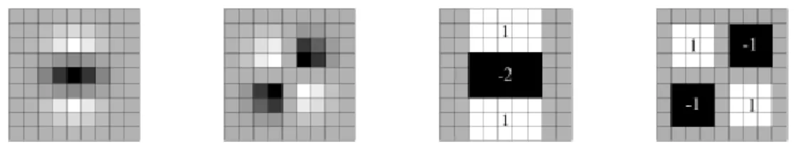
where –is the convolution of the Gaussian second order derivative with the image I in point , and similar for and . Lindeberg [9] has shown that Gausssian function is optimal for space-scale analysis but with the loss of repeatability in image rotation for multiple odds of , this applies for the Hessian based detectors too. To solve this drawback the SURF detector use the box filters (average filters) to approximate the second order Gaussian

derivatives (figure below) [10], [11].

Figure 2-9. Gaussian second order partial derivatives , and their approximations

The approximation determinant of the Hessian represents the blob response in the image at location :

( ) where

- are the blob response maps,

-

The scale space is divided into octaves. An octave represents a series of the filter response maps obtained by convolving the same input image with a filter of increasing size; an octave has in general a scaling factor of 2 and each octave is divided into constant number of scale levels.

To localise the interest points in the image and over scales, non-maximum

suppression is used than the maxima of the determinant of the Hessian matrix are interpolated.

Figure 2-10. Feature point detection using SURF.

Description and matching: SURF descriptor describes the distribution of the

intensity within the interest point neighbourhood. To achieve this approach this method follows three main steps:

1. Fix a reproducible orientation from the information in a circular region around the interest point- by calculation of the distribution of the first order Haar wavelet responses in x and y directions.

2. Construct a square region centred on the feature region with the orientation from step 1 and extract a SURF descriptor from it – based on the sum of Haar wavelet responses.

3. Matching- with a new indexing step based on the sign of Laplacian.

In order to find a dominant orientation that is invariant to the image rotation we must calculate an orientation that is reproducible. For this purpose we first calculate the Haar wavelet responses in x, y directions within a circle with radius 6s around the interest point, where s is the scale at which the interest point is detected. The sampling

step and the size of wavelets are scale dependent and have the chosen values of 4s, s respectively (see figure below) [10].

Figure 2-11. Haar wavelet filters to compute the responses in x and y direction and the sliding orientation window of size 60 degrees [10].

As the figure shows the wavelet responses are represented as points in space with horizontal and vertical response strength. The dominant response is estimated by calculating the sum of all responses within a sliding orientation window with an angel of 60 degrees, the size of sliding window must be chosen carefully. Summed

horizontal and vertical responses yield to an orientation vector and the longest vector is the dominant orientation [10].

The size of the square window is 20s and the region is split up regularly into smaller 4x4 sub-regions with 5x5 regularly spaced sample points inside. The 4x4 separation gives the best performance from the tests and preserves the important spatial

information. After computing the Haar wavelet responses dx, dy for each sub-region to increase the robustness we weight these responses with a Gaussian (ơ=3.3s) centred at the interest point. For each sub-region the wavelet responses dx, dy and their

absolute values are summed up and they form a feature vector of length 64. Hence, each sub-region has a four dimensional descriptor vector [10]

v = (∑ ∑ ∑| | ∑| | ).

For matching this algorithm uses a new fast indexing method based on the sign of the Laplacian. The sign of Laplacian distinguishes bright blobs on the dark backgrounds from the reverse situation. The blob like regions are calculated at the detection phase so there is no need for extra information while matching the features this allows a really fast matching without the loss on the performance of the descriptor. Hence, in the matching stage we only compare if features has the same contrast (sign).

-1

+1

- -1

2.3

Real-time Image Processing

Over the past decades the field of real-time image and video processing has experienced an enormous growth, a large number of related articles have been presented in various conference proceedings and journals.

Nowadays smart camera systems are providing piece of mind through intelligent scene surveillance and this is continuing to play a key role in industrial inspection systems.

Real-time image and video processing include processing vast amounts of image data in an interval of time for the purpose of extracting useful information which could mean anything from obtaining an enhanced image to intelligent scene analysis. Signals that represent digital images are multidimensional signals and are thus quite data intensive, requiring a significant amount of computation and memory resources for their processing. The amount of data increases if colour is also considered. A common challenge in real-time image processing systems is how to deal with this vast amount of data and computations. The concept of parallel processing is introduced as key solution. Efficiency of an image processing system depends on how well different forms of parallelism are implemented in an algorithm, which can be data level

parallelism (DLP) and instruction level parallelism (ILP). DLP acts in the application of the same operation on different data sets while ILP acts on scheduling the

simultaneous execution of multiple independent operations in a pipeline.

Image processing operations are traditionally classified into three main levels, namely low, intermediate and high where each level differs in its input-output data

relationships.

There are three main definitions of the concept of real-time:

 Real-time in perceptual sense: describes interaction between a human and a computer device for an instantaneous response of the device to an input by a human user. The response of the device occurs seemingly immediately, without a human user ability to sense the calculation delay.

 Real-time in software engineering sense: describes the systems that must satisfy the limited response time constraints to avoid failure. Depending on the strictness attached to the interval of response time in software engineering the systems are classified into hard real-time, firm real-time and soft real-time systems.

 Real-time in signal processing sense: is defined as completing the processing in the time between successive input samples.

Developing a real-time image processing system can be quite a challenge due to the need of computing vast amount of data in a short interval of time. A good

combination of the hardware and software approaches can end up into an appropriate solution for a specific application.

In the case of non-real time image processing all the constraints that we mentioned for real-time image processing are not part of the challenges. Here, we do the calculation without the need of giving the results in a short interval of time.

3

Simultaneous Localization and Mapping

(SLAM) Problem

In this chapter we will give a short historical introduction to the SLAM problem and the existing theoretical and practical solutions to this problem.

Next sub-part of this chapter describes the toolkit used during the case study called 3D Toolkit continuing with a brief introduction to the algorithms within the mostly used part of this toolkit called slam6d.

3.1

SLAM from a Historical Perspective

The term probabilistic SLAM has its genesis in 1986 in an IEEE conference of

Robotics and Automation held in California, the time when probabilistic methods start to be introduced in artificial intelligence field and robotics.

Simultaneous localization and mapping (SLAM) problem tries to find the solution of placing a mobile robot in an unknown environment and unknown location and for robot to incrementally build a consistent map of the environment and at the same time use this map to compute its location.

Solutions to the SLAM problem have been seen as an “impossible task” from the mobile robotics community because it will provide the possibilities to make a robot truly autonomous.

After the SLAM was introduced to the researchers a bunch of papers were produced to address many issues about the SLAM problem. At very first, these papers

recognized that consistent probabilistic mapping was a fundamental problem, there must be a high degree of correlation between the landmark observations taken by the robot while moving in an unknown environment due to the common error in estimated vehicle location. These correlations would grow with consecutive observations. A full solution for combined localization and mapping problem requires a joint state,

consisting of the vehicle pose and every landmark position to be updated for each landmark observation.

The complex nature of the SLAM problem led to the focused theoretical work in either mapping or localization as a separate problem for a while. The conceptual breakthrough came after recognition that combined mapping and localization problem, once formulated as a single estimation problem, was actually convergent. Correlations between landmarks, which most of the researches has tried to minimize were actually the most critical part of the problem, the more these correlations grow, the better the solution. Conceptually and theoretically SLAM is now considered as a solved issue, it also has been implemented in a number of different domains.

However, significant issues remain to be solved in realizing more general SLAM solutions and the use of more rich maps as a part of SLAM algorithms [12], [13]

3.1.1 Essential Formulation and Structure of the SLAM Problem

Figure 3-1. The essential SLAM problem [12].

If we consider a mobile robot that moves in an environment and at the same time it takes relative observations of a number of unknown landmarks using a sensor located in the robot as it is shown in figure 3-1. At the time instance , we can define the following:

: Vehicle location and orientation state vector

: The control vector, applied at the time to derive the vehicle to the state

at the time .

: The location vector of i-th landmark, whose true location is time invariant.

: An observation taken from the vehicle of the location of the i-th landmark at

time .

Furthermore, the following sets are also defined:

{ } { }: The history of vehicle location. { } { }: The history of control inputs.

{ } { }: the set of all observations landmark

observations.

Probabilistic SLAM problem requires that the probability distribution

|

to be computed for all times . The SLAM problem is a Bayesian form and this computation requires two models an observation model and a motion (state

transition) model.

| - describes the observation model which is the probability of making an observation when the vehicle location and landmark locations are known.

| - describes the motion model for the vehicle which is the probability distribution on state transition. From the formula we see that the next state

depends only on the previous state and the control vector .

As we see from the probability function a recursive solution for the SLAM problem is desirable for calculating the joint posterior for robot state and map m at a time k. based on all observations and control inputs including the initial state too.

SLAM algorithm is now implemented in two-step recursive form: time-update and

measurement update form [12].

Time-update form:

| ∫ | | Measurements update form:

| | | |

3.1.2 Solutions to the SLAM Problem

Now, that we have the structure of the probabilistic SLAM problem, the next step is to find the methods that can solve it. The solution was to find a good presentation for the observation and motion model that allows an appropriate computation for the time - update and measurement-update form [12].

Researchers came into two methods that could solve the SLAM problem:

 Extended Kalman Filter (EKF-SLAM) [13] – a form of state-space model

 Rao-Blackwellized Filter (FastSLAM) [12] – describes the vehicle motion model.

After these two solutions the researchers focused their work in three key areas: reduction of computational complexity, data association and environment

representation.Today, there are many approaches developed to solve the three key areas mentioned above, for more see reference [13].

Nowadays, SLAM methods have reached a considerable state of maturity. The main goal in the future is to use SLAM in areas where GPS is unavailable or unreliable like: remote planets, underwater, in urban canyons etc [13].

3.2. 3D Toolkit

This toolkit is newly developed by two universities in Germany: The School of Engineering and Science at Jacobs University and the Institute of Computer Science at University of Osnabrück [14].

This toolkit provides algorithms and methods to process 3D point clouds. All the components of this toolkit can be compiled and used with Linux, Windows and Mac OS. During my work in case study I manage to test this toolkit in Windows and Linux.

The list of components included in 3D toolkit:

 Slam6d: the component that do automatic, high-accurate registration of the scans. Merges the scans into one coordinate system.

 Show: the component that is a fast 3D viewer. This component is for visualization of .frame files generated by slam6d.

 Shapes: the component that contains shape detection algorithms in 3D point clouds with the main functionality in detecting planes.

 Scanner: the component that calculates a 3D point cloud from a video in which a laser line moves over an object.

3DTK supports a number of file formats and new formats can be added too [14]. This toolkit uses a left-handed coordinate system for internal representation. In the case study two components of this toolkit slam6d and show are used. The file format that is used is the default file format supported by 3DTK and is called scan_io_uos [14]. In the next sub-chapter we will describe more about these two components and the used file format.

3.2

Algorithms within Slam6d

As we mentioned before slam6d is one of the components of the toolkit that does scan registration. Scan registration is the process which merges the scans into one

coordinate system.

This component can register scans using two types of algorithms:

 ICP Matching: sequential matching of the scans

 Global Matching: processes multiple scans at the same time.

3.2.1 Iterative Closest Point Algorithm – ICP

ICP algorithm registers two point sets in a common coordinate system [15]. Point cloud registration is the most crucial step in 3D model constructions. ICP is the standard algorithm used for this purpose when an initial relative pose estimate is available [16]. The algorithm relies on minimizing an error function over closest point correspondences. The most difficult part when minimizing the ICP error function is to ensure the orthonormality constraint of the included rotation matrix.

If we have two independent sets of 3D points ̂ (model set) and ̂ (data set) which corresponds to a single shape, we want to find the transformation (R, t) consisting of a rotation matrix R and translation vector t which minimizes the cost function:

∑‖ ‖

The represents all the corresponding (closest) points where ̂ and ̂. Here, two main things need to be calculated: corresponding points and the transformation that minimizes on the basis of the corresponding points.

The computation of closest points is the most expensive step in ICP algorithm, using optimized k-d trees the overall cost for finding the closest points is where N is the number of generated 3D points from the point source [16].

The second thing that needs to be calculated is the transformation (R, t) that minimizes the error function of the ICP algorithm. There are four algorithms that solve the error function of the ICP algorithm in the closed form plus three other

methods that solve this problem in the linear form. All these methods are supported by slam6d when doing a sequential registration of the point clouds [16]. Most of these algorithms compute the rotation first and the translation is derived using the rotation. For calculating R separately two point sets M’ and D’ need to be calculated by subtracting the mean of the points used in matching.

{ } ; { } and ∑ ; ∑

Replacing these equations in the main error function we get the following: ∑ ‖ ⏟ ‖ _̃ ∑‖ ‖ ̃ ∑ ∑‖ ̃‖

To minimize the error function we have to minimize all the terms above. From the equation we see that the second term is zero, since it depends all from centroids. The third term has it minimum at ̃ or . Now, the algorithm depends

from the first term only and needs to minimize only that term. It is also expressed in terms of rotation only.

∑‖ ‖

As we mention before here we have four methods to calculate rotation matrix in a closed – form solution, all are non-linear:

1. This method uses singular value decomposition (SVD) for calculating R [17]. For a given 3x3 correlation matrix H:

∑ ₍ )

where

∑ , ∑ , ....

The optimal solution for the rotation R is represented as an orthonormal 3x3 matrix this calculation is derived from the SVD of the

cross-correlation matrix H where [16], [17].

2. This method is similar to the first one, a correlation matrix H same as before is calculated even here. After this a polar decomposition is computed H=PS, where _{. For this polar decomposition a square root of the matrix} is defined [18]. Here the rotation matrix is given by equation:

(

√ √ √ )

where { } are the eigenvalues and { }are the corresponding eigenvectors of matrix [16], [18].

3. This method uses something that is called unit quaternion to find the

transformation (R, t) for the ICP algorithm. Here, the rotation is represented as a unit quaternion ̇, that minimizes is the largest eigenvalue of the cross-covariance matrix. For more details see reference [16], [19].

4. The fourth method that minimizes the cost function for the ICP algorithm uses the so-called dual quaternions. Unlike the other methods here the

transformation is found in a single step, there is no need to compute the rotation separately. The optimal solution for the transformation is again a non-linear solution which depends on eigenvalues [16], [20].

3.2.1.1 Linearized Solutions to ICP

So far, we have discussed the closed-form solutions for minimizing the cost function of the ICP algorithm and they were all non-linear. Some linear solutions are presented at al. [16] that can solve the ICP transformation and also can be used in global

matching.

Most of these linear methods are constructed under the assumption that the

transformation (R. t) that needs to be calculated by ICP is very small which allows doing different approximation for going from non-linear to linear solutions. Here comes a brief description of these methods:

1. Registration using helix transform: this method approximates the solution by using instantaneous kinematics which computes the displacement of a 3D point by a related transformation via helical motion. For more details refer to [16], [21].

If v(p) is a displacement of a 3D point p, given by the parameters ̅ , i.e. ̅ . In the case of error function the displacement of the points in D has to minimize the distance between the point pairs. Thus, the error function can be rewritten in the form:

̅ ∑‖ ( )‖

∑‖ ̅ ‖

As we see now the error function is a quadratic function with the two

unknown variables ̅ , the optimal displacement of this equation is given by solving the following linear system: ̅ , where

̅ .

2. Small angle approximation: this method is based on small angle approximation. The rotation matrix R is given based on Euler angles:

(

)

After this the first order Taylor series approximation that is valid for small angels is used to simplify the expression of the rotation matrix:

=> ( )

As a second approximation is assumed that the result of a multiplication of small angels is even smaller value that can be omitted. Than the rotation matrix will be:

(

)

From rotation matrix R we see that it’s no longer orthonormal, we need to replace it again in the formula for E(R. t) and use the centroids to find the finale solution [16].

3. Uncertainty – based registration: this method calculates the uncertainty of the poses calculated by the registration algorithm. Calculation of the pose

uncertainty can be done using two methods: uncertainty based with Euler angles and with quaternion. For more details see reference [16].

3.2.2 Global Matching

While using the ICP algorithm for registering several 3D data sets errors sum up due to imprecise measurements and small registration errors, next issue while using ICP is the loop closing when the robot returns to a location that it has been before it can be that the resulting map is incorrect. ICP algorithm does a sequential matching by using pair wise scans. Global matching does match n-scans at the same time, it reduce the error function at one step and removes the loop closing problem [16], [22].

Here, all new scans are registered against so-called metascan, which is the union of the previously acquired and registered scans. This method is order dependent and does not spread out the error. The ICP error function is replaced with a global one:

∑( ̅ )

( ̅ )

where ̅ models random Gaussian noise, is a Gaussian distributed error with zero mean and a covariance matrix computed from closest point pairs. Solution to this global error function is given by Lu and Milios at [23] and extended to 6DoF at [22]. All the above mentioned linearized methods for the ICP algorithm can be implemented for the global registration of the n-scans too.

1. Global registration using the helix transform.Here the error function for global matching is extended to include all poses ( ̅ ) , where j presents a set of point pairs with j as the model set and k as data set. The error function including all poses will be [16]:

∑ ∑ ( ( ̅ ) ̅ )

This error function can be solved after some reformulations according to reference [16].

2. Global registration using the small angle approximation. Similar to helix

transform even here the error function is extended to include all poses: ∑ ∑| |

Using the centroids and where , . By substituting this to the above error function we get the following:

∑ ∑| ( )|

Now we continue the calculation by using the binomial theorem in which the last two terms will be equal to zero because all values refer to centroids. Like previously in the ICP algorithm this will allow us to solve for the rotation of all poses independent from their translation, for more details refer to [16].

3. Uncertainty –based global registration. Here the global error of all poses will

be described as:

∑( ̅ ) ( ̅ )

where ( ̅ ) is the Gaussian distribution of the error between two poses. Just like in the ICP pair matching case calculation of the pose uncertainty can be done using uncertainty based with Euler angles or with quaternion. For more details see reference [16].

3.3 The SHOW Component of 3DTK

As we mentioned before this is the component that shows results after matching with the slam6d. For showing the results the show component needs .frame files that are generated from slam6d, these files consist of the transformation computed from the point matching. To visualize .frame files, we must specify the folder which contains the scans in command line. Successful running of the show component will open three windows:

 3D_Viewer

 3D_Viewer - Controls

 3D_Viewer Selection.

Selecting the control window allows us to navigate in the main view window and change the appearance. Selection window can be used to select point size, fog density, camera path, color of the points. Nowadays, modern hardware and software generates a huge amount of 3D points at a very high rate therefore visualization of this data requires processing of a massive amount of 3D data. Show uses so-called octree to store and compress the data efficiently and precisely. An octree is a tree data structure that is used for storing 3D point clouds, is an extension of binary and quad trees which stores one and two dimensional data. Octrees subdivide the point clouds into spatial regions and as a result of this the visualization speed is increased, for more details about the octree and algorithms inside Show component see [14], [24].

4

Research Methods

This chapter shortly describes the used research method and data collection methods.

4.1

Case Study Research

The main goal with this project was to find the best alignment of 3D feature point images using a SLAM solution. Image processing field by its nature is a complex field and time consuming when working with it. Having into consideration the time

limitation for this project I decided to do a case study [25], [26] and use 3DTK especially slam6d to do the matching (registration) of 3D feature point stereo images. Slam6d has been developed to do point cloud registration, that are generated using 3D laser scans or generally laser scans. Here point clouds are called feature points and they are generated by using a stereo camera and the algorithms behind the IBGN system developed by the STS Company.

Since, 3DTK is designed for matching point cloud laser scans the results of scan registration using slam6d are quite accurate and good for in and outdoor

environments. In this case study we will explore how good is slam6d for registering 3D point cloud images that are not generated by 3D laser scans but instead the 3D point cloud images are generated by a different technique than laser scans.

The case is to implement slam6d for registering 3D feature point images and evaluate the results based on the scenarios:

 Stationary 3D image sensor, single image.

 Moving 3D image sensor (known movement), multiple images.

 Consecutive movement of 3D image sensor following a trail.

 Consecutive movement of 3D image sensor following a loop, thus needing to integrate with old image points.

This case study is built upon the work of others but is going to elaborate and test slam6d in a manner that is not explored previously. By means of this case study we want to answer the questions below:

 How accurate is slam6d for registering a single 3D feature point image?

 How accurate is slam6d for registering multiple images when moving the camera?

 Why the registering results using slam6d are good (erroneous)?

4.1.1 Data Collection Methods

One of the weaknesses of the case study methodology is that there is no strict rule for collecting and analyzing the data. As a result of this weakness, three methods to collect the data and the needed information for the work have been used:

 Literature review

 Experiments (Tests)

Literature review: In order to give your research a good theoretical framework and a

good starting point this is the method that is required in almost every research work. have also given a general theoretical background in the computer vision field and some of the algorithms for detecting and matching feature points.

Interviews: To use interviews when doing a case study research is quite common but

interviews are quite frequently used in other research methods too.

During this project interviews have been carried out with two engineers from the STS that work with the IBGN project and image processing in vision applications. The interviews were individual with each engineer and very open with non-limited length and they had the nature of a dialog or conversation. The main purpose with these interviews was to help me get more familiar with the project and to be able to understand the goal with this project. Interviews were held continuously and they made it easier to have a better communication with the company engineers and to continuously follow the progress of the project. These interviews were recorded which made it easier to concentrate on the conversation instead of taking notes during the conversation.

Experiments (Tests): The STS Company provided the test data which are used in the

case study as input data to the slam6d and the results are analyzed.

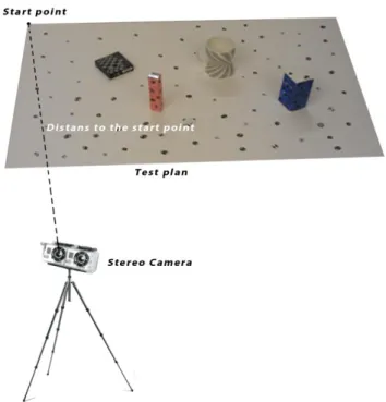
4.2

Test Plan

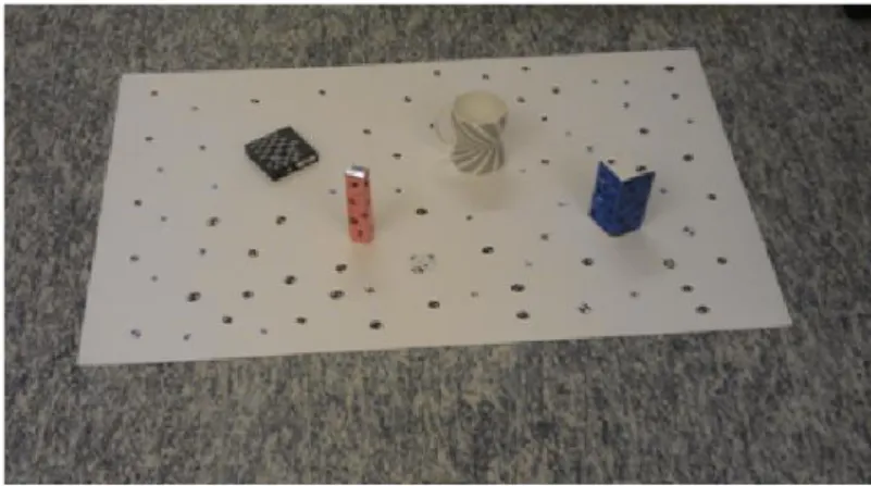
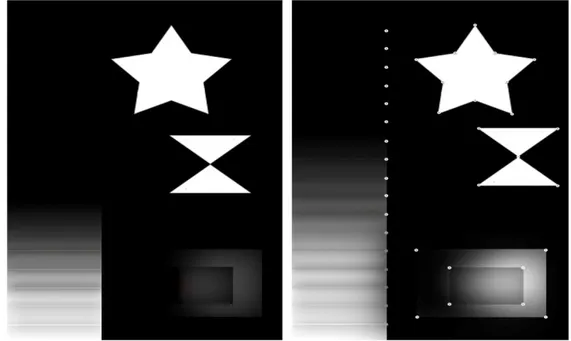
During the interview conversations with the engineers at STS we came into conclusion to make a kind of experimental set up or test plan that could be used to capture images and generate the 3D feature point images. The test plan is made by a carton paper with dimensions of 50cm x 40cm and it has some 3D objects glued in its surface, as it’s shown in the figure below.

Figure 4-1. Test plan used to get the experimental data.

The main reason for using this test plan was because of the fact that this will make it easier to capture and analyse the matching results of feature point images when we have full control of the entire test plan and the objects on the test plan.